Distinguishing among Scalar Field Models of Dark Energy

Abstract

We show that various scalar field models of dark energy predict degenerate luminosity distance history of the Universe and thus cannot be distinguished by supernovae measurements alone. In particular, models with a vanishing cosmological constant (the value of the potential at its minimum) are degenerate with models with a positive or negative cosmological constant whose magnitude can be as large as the critical density. Adding information from CMB anisotropy measurements does reduce the degeneracy somewhat but not significantly. Our results indicate that a theoretical prior on the preferred form of the potential and the field’s initial conditions may allow to quantitatively estimate model parameters from data. Without such a theoretical prior only limited qualitative information on the form and parameters of the potential can be extracted even from very accurate data.

I Introduction

One of the standard methods of interpreting the growing body of evidence from supernovae data and other measurements that the expansion of the Universe is accelerating, is to assume the existence of a dark energy component and to model it using scalar fields (for a recent review see fund ). This links the expansion history of the Universe to theories of fundamental physics. For example, from this perspective the value of the potential at its minimum is the cosmological constant (CC). Since at this point there are many theoretical ideas about the form of the potential but none that particularly stands out, it would have been helpful if the data from cosmological measurements, such as supernovae Ia, CMB and various others, could provide hints about some generic features of the potential.

Viable scalar field models of dark energy need to have potentials whose energy scale is about the critical density $\sim 10^{-12}{\rm eV}^{4}$, and typical scalar field masses about the Hubble mass $m\sim 10^{-33}$ eV. In such models typical scalar field variations are about Planck scale $m_{p}\sim 10^{19}$ GeV, and typical time scales for such variations are about the Hubble time $1/H_{0}\sim 10^{18}$ sec. Whether, and how well, it is possible to determine the parameters and form of potentials and the field’s dynamical history and future from data beyond such qualitative estimates has been addressed previously Chiba ; Barger ; weller ; Ng ; Bludman ; Eriksson ; hut ; star1 ; efst . Weller and Albrecht weller concluded that some potentials could be differentiated using SNAP-like data snap . They approximated the equation of state (EOS) of each of the models, and showed by likelihood analysis that some of the models are distinguishable. Another approach is “reconstruction” hut ; star1 ; efst . Here one rewrites the potential as a function of the luminosity-distance ($d_{L}$) and its derivatives, which are in turn functions of the redshift. The potential (and not the EOS) is approximated by a fitting function, and statistically tested against a set of accurate $d_{L}$ measurements. The efficiency of reconstruction depends on the accuracy of knowing the values of $\Omega_{m}$ (this is needed also when one fits the EOS), and $H_{0}$ (this is needed only for reconstruction).

On general grounds we expect that scalar field potentials are less distinguishable than their corresponding EOS, because different potentials, with properly adjusted initial conditions for the field can produce very similar EOS.

In previous papers m1 ; m2 we have found that supernovae (SN) measurements are limited as a probe of the dark energy EOS $w_{Q}$, due to degeneracies. Specifically, it was shown that $d_{L}$’s corresponding to two different $w_{Q}$’s are degenerate if both EOS coincide at some point at a relatively low red shift, $z^{*}$ (see also sweetspot and astier ). The purpose of the present analysis is to explore the implications of this degeneracy on the possibility to determine the scalar field potential. For a given functional form of potential, we would like to quantify the amount by which the parameters of the potential can be varied, and still be indistinguishable by accurate SN measurements. Our criteria for indistinguishability between two models is that their resulting $d_{L}$’s differ at most by 1% up to redshift $z=2$, in accordance with the anticipated accuracy of future SN measurements. In addition, we would like to determine whether the functional form of the potential can be distinguished or constrained by data.

We look for degeneracies among potentials using the following procedure: For a given class of potentials, we change the parameters as well as the initial values of the field, with the constraint that $w_{Q}$ at $z^{*}$ remains unchanged. This results in models whose $w_{Q}$ cross at $z^{*}$. We know from our previous analysis that in this case the models tend to be degenerate. Then we evaluate numerically the differences in the $d_{L}$’s of the models to verify this.

There are additional sources of degeneracy that we do not consider here. In our procedure the value of the potential energy and the value of the kinetic energy remain unchanged. Allowing changes in the potential that are compensated by changes in the initial conditions for the kinetic energy will give another dimension of degeneracy. Variation in the value of $\Omega_{m}$ is yet another degree of freedom, as is relaxing the assumption of a flat Universe and considering the effects of a clumpy Universe sps . Additionally, the value of $z^{*}$ in different models can be shifted. We have found that $z^{*}$ varies slowly with the red shift depth of the data set, $z_{max}$. The dependence is approximately linear $z^{*}=\alpha z_{max}+\beta$ (see also linder ), $\alpha$ and $\beta$ are model dependent but $\alpha$ is typically small, about 0.2. And, finally, we have looked only at a class of simple potentials that have two independent parameters. Additional parameters in the potential yet again open up new degrees of freedom, each of which increases the degeneracy of each of the parameters. Since we have found that this class of simple potentials suffers from large degeneracies, we see no phenomenological justification for using more complex potentials. If a theoretical prior about the form of the potential and initial conditions can be motivated then some of this degeneracy can be removed.

II Degeneracies of scalar field potentials

We consider a flat Universe with non-relativistic matter (dark matter included) whose EOS is $w_{m}=0$, and a dark energy component which we model by a canonically normalized and minimally coupled scalar field. Einstein’s equations for such a Universe are the following,

$$H^{2}=\kappa^{2}\left(\rho_{m}x^{3}+\frac{1}{2}x^{2}H^{2}\phi^{\prime 2}+V(\phi)\right)$$ (1)

$$xHH^{\prime}=\frac{3\kappa^{2}}{2}\left(\rho_{m}x^{3}+x^{2}H^{2}\phi^{\prime 2}\right)$$ (2)

$$x^{2}H^{2}\phi^{\prime\prime}+(x^{2}HH^{\prime}-2xH^{2})\phi^{\prime}+\frac{dV}{d\phi}=0,$$ (3)

where $x=1+z$, $\kappa^{2}=\frac{8\pi}{3m_{p}^{2}}$, $\rho_{m}$ is the matter energy density today, primes denote derivatives with respect to $x$, and $V$ is the potential of the scalar field. The scalar field’s EOS ($w_{Q}$) is given by,

$$w_{Q} = \frac{p_{Q}}{\rho_{Q}}$$ (4)

$$= \frac{x^{2}H^{2}\phi^{\prime 2}-2V}{x^{2}H^{2}\phi^{\prime 2}+2V}.$$

We choose a model, and vary the parameters of the potential $P_{i}$, as well as the values of the scalar field at $z^{*}$ keeping its derivative constant,

$$\phi(z^{*}) \rightarrow \phi(z^{*})+\delta\phi$$ (5)

$$V \rightarrow V+\delta V(P_{i},\delta P_{i},~{}\delta\phi)$$ (6)

$$\delta\phi^{\prime}(z^{*}) = \delta H(z^{*})=\delta\rho_{m}=0.$$ (7)

These variations result in variations in eqs.(4) and (1):

$$w_{Q}+\delta w_{Q} = \frac{x^{2}H^{2}\phi^{\prime 2}-2(V+\delta V)}{x^{2}H^{2}\phi^{\prime 2}+2(V+\delta V)}$$ (8)

$$\approx w_{Q}+\left[\frac{2(1+w_{Q})}{x^{2}H^{2}\phi^{\prime 2}+2V}\right]\delta V+{\cal O}(\delta V^{2})$$

$$H^{2} = \kappa^{2}\left(\rho_{m}x^{3}+\frac{1}{2}x^{2}H^{2}\phi^{\prime 2}+(V(\phi)+\delta V)\right).$$ (9)

In eq.(8), we have kept terms up to first order in $\delta V$, assuming it is small enough.

Since we know that if the values of $w_{Q}(z^{*})$ are equal for two models then their luminosity-distance history is approximately degenerate, we explore part of the degeneracy in parameter space by requiring that $\delta w_{Q}(z^{*})$ vanishes. In eq. (8) we ignore higher orders in $\delta V$, so we simply require that $\delta V$ vanishes to first order. On the other hand, even a small deviation from a spatially flat cosmology will be amplified by the evolution of the solution. We therefore need to require that eq. (9) holds exactly.

The two constraints we are imposing are then

$$\delta V(P_{i},\delta P_{i},~{}\delta\phi)^{(1)}=0$$ (10)

$$\delta V(P_{i},\delta P_{i},~{}\delta\phi)^{(exact)}=0.$$ (11)

This set of variations and constraints is algebraic and can often be solved analytically. The analytical solution connects any given model to a family of associated models, all of which have the same $w_{Q}$ at $z^{*}$. The next step is to check numerically how large are the allowed parameter variations such that different models in the family are indistinguishable.

Initial conditions are given at $z^{*}$, but the evolution of each of the models towards $z=0$ is different, and they end up with a different value of $H_{0}$ (Hubble parameter at $x=1$, $z=0$). To ensure that all models have the same value of $H_{0}$ we rescale them,

$$\widetilde{H}=\frac{H}{H_{0}},~{}~{}\Omega_{m}=\frac{\rho}{H_{0}^{2}m_{p}^{2}},~{}~{}\widetilde{\phi}=\frac{\phi}{m_{p}},~{}~{}\widetilde{V}=\frac{V}{H_{0}^{2}m_{p}^{2}}.$$ (12)

Equation (1) can be reexpressed in terms of the rescaled variables

$$\widetilde{H}^{2}=\Omega_{m}x^{3}+\frac{1}{2}x^{2}\widetilde{H}^{2}\widetilde{\phi}^{\prime 2}+\widetilde{V}.$$ (13)

This means that although initially only the scalar field potential energy is varied, eventually all quantities (except $H_{0}$) may vary between models. As we shall show later (section III), it turns out that differences in $\Omega_{m}$ are negligible. This result is not surprising: as was shown in m2 (see in particular Fig. 2), this type of degeneracy characterizes models with fixed values of $\Omega_{m}$. Families of models which are degenerate with respect to SN measurements but have different values of $\Omega_{m}$ do not exhibit the enhanced resolution of $w_{Q}(z^{*})$. This means that on top of the degeneracy that we will be exploring here, another dimension of degeneracy will open up once the uncertainties in $\Omega_{m}$ are taken into account. The method described here therefore exposes only part of the degeneracy among potentials.

III Degeneracies among simple potentials

We have analyzed various forms of potentials with two parameters. For all such potentials there are three independent variations, two parameters and the initial condition for $\phi$. Enforcing the two constraints eqs. (10),(11) results in a solution which is a curve in a three-dimensional space. Obviously the degeneracy is larger when more parameters are allowed.

One class of potentials we have looked at is $V(\phi)=\frac{1}{2}m^{2}\phi^{2}+v_{0}$. This is one of the standard simple forms of potentials, $m$ is the scalar field mass, $v_{0}$ is the value of the potential at the minimum (the CC). As explained previously we already have an order of magnitude estimates for $v_{0}$ and $m$, but we would like to know whether they can be determined in a more quantitative and conclusive way by the data. In particular we would like to know whether it is possible to distinguish models with a vanishing CC ($v_{0}=0$) from models with a non-vanishing CC ($v_{0}\neq 0$). For this class of quadratic potentials the variation is given by:

$$V+\delta V = \frac{1}{2}(m+\delta m)^{2}(\phi+\delta\phi)^{2}+(v_{0}+\delta v_{0})$$ (14)

$$= \left[\frac{1}{2}m^{2}\phi^{2}+v_{0}\right]+\left[m^{2}\phi\delta\phi+m\phi^{2}\delta m+\delta v_{0}\right]$$

$$+ \left[\frac{1}{2}(m\delta\phi+\phi\delta m)^{2}+\delta\phi\delta m(m+\delta m)(\phi+\delta\phi)-\frac{1}{2}\delta m^{2}\delta\phi^{2}\right].$$

The first bracket is $V$ itself. The second bracket is $\delta V^{(1)}$ which should vanish, and the last bracket is $\delta V^{(exact)}-\delta V^{(1)}$ which should vanish as well. The solution is a curve in the $(\delta v_{0},~{}\delta m,~{}\delta\phi)$ space. On this curve changes in the curvature and the height of the minimum of the potential are compensated by a change in the value of $\phi$ such that the potential energy of the field is locally unchanged.

Figure 1 shows a variety of quadratic potentials on the left, their resulting $w_{Q}$ in the middle, and the relative difference in $d_{L}$ on the right. The parameters of the potentials are listed in table I. Notice that although the fiducial model has a vanishing CC, $v_{0}=0$, it is degenerate with models that have $v_{0}$ of order unity in units of the critical density ($m_{p}^{2}H_{0}^{2}$). The uncertainty in $m$ is of order unity in units of the present value of the Hubble parameter $H_{0}$.
All the models have values of $\Omega_{m}$ which are within $\pm 0.01$ from the value of the fiducial. This means that we are indeed exploring here the degeneracy due to the integral relation between $d_{L}$ and $w_{Q}$, and not the degeneracy due to the uncertainty in $\Omega_{m}$. As explained previously, this is a direct consequence of our method.

Following the same procedure we have analyzed other popular classes of potentials with two parameters. Figure 2 shows similar results for an exponential potential, $V=Ae^{-B\phi}$. For this specific potential only some of the solutions of eqs. (10) and (11) can be found analytically, hence the degeneracy shown is a smaller than the full degeneracy, as can be seen by the reduced range of allowed values of $A$ in table II. Figure 3 shows the results for an inverted quadratic potential, $V=-\frac{1}{2}m^{2}\phi^{2}+v_{0}$.

As can be seen from the figures, the deviation in $d_{L}$ tends to peak at low redshift, about $z=0.4$. This results from the following reason: consider two models whose EOS cross at $z=z^{*}$. For redshifts $z<z^{*}$, the different $w_{Q}$ of the models imply different rates of expansion. The model whose $w_{Q}$ is more negative will expand faster, making the $d_{L}$’s of the two models diverge. In the range $z>z^{*}$ the trends reverse, making their $d_{L}$’s converge. If this were the only source of degeneracy among models, it would have been useful to focus measurements in this range of redshifts, $z\sim 0.4$. Unfortunately a second degeneracy (due to the uncertainty in $\Omega_{m}$) degrades the extra sensitivity in this region of redshifts.

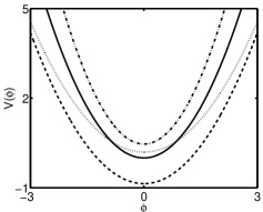
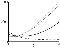
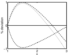
Figure 1: Various quadratic potentials (shown on the left), their resulting $w_{Q}$ (middle), and the relative difference in $d_{L}$ (right). The parameters of the potentials are listed in the table I.

	Solid (fiducial)	Dashed	Dotted	Dash-dotted
$\bf{(\frac{m}{H_{0}})^{2}}$	1.51	1.12	0.98	1.99
$\bf{\frac{v_{0}}{m_{p}^{2}H_{0}^{2}}}$	0	-0.86	0.20	0.47
$\bf{\Omega_{m}}$	0.30	0.31	0.29	0.29

Table 1: Parameters of quadratic potential plotted in Figure 1.

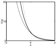
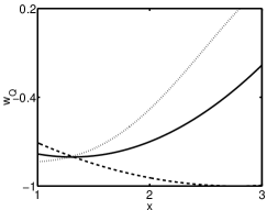
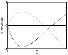
Figure 2: Various exponential potentials (shown on the left), their resulting $w_{Q}$ (middle), and the relative difference in $d_{L}$ (right). The parameters of the potentials are listed in table II.

	Solid (fiducial)	Dashed	Dotted
$\bf{\frac{A}{m_{p}^{2}H_{0}^{2}}}$	4.43	4.13	4.12
$\bf{m_{p}B}$	1.78	2.40	1.36
$\bf{\Omega_{m}}$	0.30	0.30	0.29

Table 2: Parameters of exponential potential plotted in Figure 2.

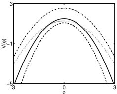
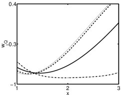
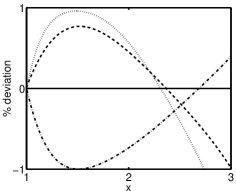
Figure 3: Various inverted quadratic potentials (shown on the left), their resulting $w_{Q}$ (middle), and the relative difference in $d_{L}$ (right). The parameters of the potentials are listed in table III.

	Solid (fiducial)	Dashed	Dotted	Dash-dotted
$\bf{(\frac{m}{H_{0}})^{2}}$	1.51	1.88	0.98	1.08
$\bf{\frac{v_{0}}{m_{p}^{2}H_{0}^{2}}}$	1.51	1.09	1.28	2.55
$\bf{\Omega_{m}}$	0.30	0.29	0.29	0.31

Table 3: Parameters of inverted quadratic potentials plotted in Figure 3.

So far we have analyzed the uncertainty in determination of parameters under the assumption that the form of the potential is known. Without a theoretical prior on the form of the “true” potential it is important to find whether different classes of potentials can be distinguished by the data alone. We will present here only a representative example and not attempt a systematic analysis to expose the full degeneracy.

In Figure 4 we show an example of four different degenerate potentials. All models have $\Omega_{m}=0.30$. The potentials we have used in this example are $V=\frac{1}{2}m^{2}\phi^{2}+v_{0}$ (solid), $V=Ae^{-B\phi}$ (dotted), $V=-\frac{1}{2}m^{2}\phi^{2}+v_{0}$ (dashed), and $V=a+b\phi$ (dash-dotted). The right panel shows that the relative differences in their $d_{L}$’s are less than one percent up to $z=2$. The left panel shows the potentials. Although the functional forms of the potentials are very different and they do not have the same asymptotic behavior, they are nevertheless indistinguishable. This can be understood by observing that the patch of potential that was probed by the field during the relevant redshift range, (marked in the figure by the shaded area) is rather small. In this patch, differences among the various potentials are marginal.

The fact that a small patch of the potential is actually being probed justifies the use of a simple potential with a small number of parameters. A fast rolling field would have served as a better probe of the potential since it would have covered a larger patch in a given redshift range, but this would have meant a more positive $w_{Q}$ which goes against the evidence of accelerated expansion. Another possible way to enlarge the size of the probed potential patch would have been to measure $d_{L}$ over a larger redshift range. The difficulty here is that at deeper redshifts the contribution of dark energy to the total energy of the Universe is smaller, and its effects become harder to detect.

Our results may seem to disagree with those of weller , where it was shown that different forms of potentials could be distinguished using SNAP-like data alone, but we believe that they are in fact in full agreement. Our interpretation of the results of weller is that they depend on the choice of specific parameters and initial conditions for each of the potentials that makes them distinguishable. This does not mean that for a given set of data, it will be possible to determine that a specific class of potentials is preferred over another. It is quite easy to construct counter examples by choosing the potentials to look similar in the relevant redshift patch. A representative example is shown in Fig. 5. The potentials that are used here are the pseudo-Nambu-Goldstone boson potential, $V=M^{4}(\cos(\phi/f)+1)$ (with $M^{4}/(m_{p}^{2}H_{0}^{2})=0.82$ and $f/m_{p}=0.6$), and the pure exponential, $V=Ae^{-B\phi}$ (with $A/(m_{p}^{2}H_{0}^{2})=4.43$ and $m_{p}B=1.78$).

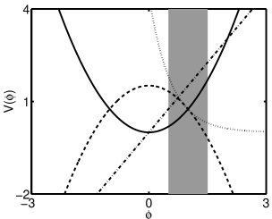
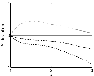
Figure 4: Various potentials (left panel), and their relative $d_{L}$ differences (right panel). The potentials we have used in this example are $\frac{1}{2}m^{2}\phi^{2}+v_{0}$ (solid), $Ae^{-B\phi}$ (dotted), $-\frac{1}{2}m^{2}\phi^{2}+v_{0}$ (dashed), and $a+b\phi$ (dash-dotted). All models have $\Omega_{m}=0.30$. The shaded area in the figure on the left indicates the region in which the field moves in the relevant redshift range, $0\leq z\leq 2$.

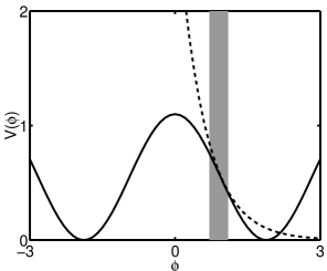
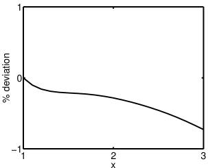
Figure 5: Two potentials (shown on the left), and their relative $d_{L}$ differences (right). The potentials we have used in this example are $v=M^{4}(\cos(\frac{\phi}{f})+1)$ (solid), and $Ae^{-B\phi}$ (dashed). Both models have $\Omega_{m}=0.30$. The shaded area in the left panel indicates the region in which the field moves in the relevant redshift range, $0\leq z\leq 2$.

IV Considering CMB

An additional measurement that can possibly probe the dark energy EOS and the scalar field potential is that of the cosmic microwave background (CMB) anisotropy. This measurement is expected to be improved with the upcoming MAP and PLANCK missions.

Using the CMB measurements to probe scalar field models requires additional theoretical assumptions about the evolution in the range from $z\sim 2$ to $z\sim 1000$. For example, that the potentials are “tracker” potentials Zlatev , or that the scalar field has negligible influence above some redshift (say, $z=2$).

It is well-known that the EOS cannot be determined using CMB anisotropy data alone due to degeneracies. A thorough analysis was done in huey , who concluded that this degeneracy persists after combining CMB and SN measurements. In m2 it was shown that the inclusion of CMB constraints in the analysis of the dark energy EOS does improve the resolution somewhat, but not significantly.

In a simple minded estimate here, we would like to show that under reasonable assumptions, CMB measurements will not help to significantly constrain the potential either. Rather than performing an extensive numerical search, as in m2 ; copeland ; fhlt , we use a different strategy: we treat CMB measurements as effectively providing one additional point on the Hubble diagram at the last scattering redshift $z_{ls}\sim 1000$. The method cannot provide numerically accurate results, but it does highlight the theoretical degeneracy that limits the ability of CMB measurements to constrain the parameters and functional form of the potential.

Treating the CMB measurements as effectively one additional point on the Hubble diagram at redshift $z\sim 1000$ can be implemented in a simple way because the angular distance and the luminosity distance are related to each other $d_{L}=(1+z)^{2}d_{A}.$ The observed angular size of any feature in the CMB, $\theta$, is related to its physical size $d$ by the angular distance $d_{A}$ to last scattering surface, $\theta d_{A}=d$. The CMB spectrum yields a series of acoustic peaks, located at $l_{n}=\frac{n\pi}{S}d_{A}$, $n$ being an integer, and $S$ is the sound horizon at last scattering surface. We are going to ignore uncertainties in the sound horizon $S$, which depends on the composition of the universe at last scattering surface.

To estimate the measurement accuracy of the CMB point on the Hubble diagram we may treat the position of the first peak $l_{1}$, as a direct measurement of the angular distance, therefore the relative errors in $l_{1}$ and in the angular distance are equal $\frac{\Delta l_{1}}{l_{1}}=\frac{\Delta d_{A}}{d_{A}}$. The position of the first peak is already measured rather well, to about $3\%$ at the $1\sigma$ level (see, for example, hu ). This is expected to be somewhat improved by MAP and PLANCK, so we may expect eventually a $3\sigma$ error in the few percent range.

Another way of estimating the accuracy of the CMB point is to use the results of m2 , where it was shown that for models which have a linear $w_{Q}$ for $z<2$ and $w_{Q}=const.$ from $z=2$ to last scattering surface, a derivative as large as $w_{1}=\pm\frac{1}{6}$ could not be distinguished at the $3\sigma$ level, assuming full sky coverage and cosmic variance limited measurement. This means that the most accurate CMB measurements do not distinguish models which lead to a difference of (+1.6%, -3.2%) in their $d_{L}$’s. Thus a $3\sigma$ measurement error estimate of a few percent in $d_{L}$ seems reasonable.

According to the preceding discussion we may define models to be indistinguishable by the CMB if their $d_{L}$ difference is less than a few percent at $z_{ls}$. We may check now whether this imposes additional constraints on our models. We find that it does, but not to a significant degree.

Since our toy models are not strictly chosen as tracker models, evolving the equations of motion backwards from $z\sim 0.3$ up to $z\sim 1000$ gives nonsensical results, the dark energy typically becomes dominant, with $w_{Q}$ approaching 1. In order to to avoid such undesirable and observationally excluded behavior, the potential needs to be changed in the regions that are probed by the field in the redshift range $z\gg 1$ such that the kinetic energy remains acceptably small, so that $w_{Q}$ remains negative and $\Omega_{Q}$ becomes sub-dominant.

Instead of building the potential piece-wise, we have chosen another approach in the spirit of m2 : we let the equations of motion evolve until $z=2$ (the redshift range relevant to SN measurement), and for $z>2$ we put by hand $w_{Q}=0$ for all models. We then calculate numerically the relative differences in $d_{L}$ at $z=1000$. Our cutoff procedure changes the $z$-dependence of $w_{Q}$ at a value of $z$ where the dark energy density is negligible, which makes the details of the $z$-dependent cutoff unimportant. We expect other cutoff procedures to give similar results.

We find that the relative differences in $d_{L}$ for our models are within a few percent, in agreement with the semi-analytic argument that we present shortly. For the potentials shown in Fig. 4, we find $\frac{\Delta d_{L}}{d_{L}}=$ $-0.9$% for the exponential potential, $-3.4$% for the inverted quadratic potential, and $-1.6$% for the linear potential. As explained previously this is just at the limit of CMB resolution. For the quadratic potential examples in Fig. 1 we find the following $d_{L}$ differences from the fiducial, dashed: $2.5$%, dot-dashed: $-6.2$%, dotted: $8.0$%, for the exponential potentials of Fig. 2 we find: dashed: $4.5$%, dotted: $6.8$%, and for the inverted quadratic potential of Fig. 3 we find dashed: $-7.8$%, dotted: $-8.1$%, and dot-dashed: $5.1$%.

For most of the models we see that CMB is expected to further constrain the parameters if the form of the potential is known. The larger $d_{L}$ differences are for models whose differences at $z\sim 2$ are larger, in agreement with the following semi-analytic argument. Given the approximate nature of our measurement accuracy estimate, the large number of additional sources of degeneracy that we have neglected, and the additional theoretical assumptions that go into the analysis with the CMB point added it is not possible, and we believe that it is not necessary to determine in a more quantitative way the amount by which the degeneracy is reduced.

We may estimate in a rough semi-analytic way the relative errors in $d_{L}$ at $z\sim 1000$ as follows. Luminosity distance at $1+z_{ls}=x_{ls}\approx 1000$ for models with $w_{Q}(x>3)=0$ is given by m2 ,

$$d_{L}(x_{ls}) = x_{ls}\sqrt{1+g}\int_{1}^{x_{ls}}\frac{dx}{x^{3/2}}\left(g+exp(3\int_{1}^{x}w_{Q}\frac{dy}{y})\right)^{-1/2}$$ (15)

$$= x_{ls}\sqrt{1+g}\int_{1}^{3}\frac{dx}{x^{3/2}}\left(g+exp(3\int_{1}^{x}w_{Q}\frac{dy}{y})\right)^{-1/2}$$

$$+ x_{ls}\sqrt{1+g}\int_{3}^{x_{ls}}\frac{dx}{x^{3/2}}\left(g+exp(3\int_{1}^{x}w_{Q}\frac{dy}{y})\right)^{-1/2}$$

$$= \frac{x_{ls}}{3}d_{L}(3)+x_{ls}\sqrt{1+g}\int_{3}^{x_{ls}}\frac{dx}{x^{3/2}}\left(g+exp(3\int_{1}^{3}w_{Q}\frac{dy}{y})\right)^{-1/2}$$

$$= \frac{x_{ls}}{3}d_{L}(3)+2x_{ls}\left(\frac{1}{\sqrt{3}}-\frac{1}{\sqrt{x_{ls}}}\right)\left(\frac{1+g}{g+exp(3\int_{1}^{3}w_{Q}\frac{dy}{y})}\right)^{1/2},$$

where $g$ is the current ratio of matter to dark energy densities, and we have set $H_{0}$ to unity. The second term can be expressed in terms of the luminosity distance at $x=3$ and its derivative:

$$\left(\frac{1+g}{g+exp(3\int_{1}^{3}w_{Q}\frac{dy}{y})}\right)^{1/2}=3^{3/2}\frac{d}{dx}\left(\frac{d_{L}}{x}\right)_{x=3},$$ (16)

so,

$$d_{L}(x_{ls})\simeq-\frac{x_{ls}}{3}d_{L}(3)+2x_{ls}d_{L}^{\prime}(3).$$ (17)

Now we would like to examine the difference in $d_{L}(x_{ls})$ for two models. For a simple and rough error estimate, we may use $d_{L}^{\prime}(3)=c_{1}\frac{d_{L}(3)}{3}$ and $\Delta d_{L}^{\prime}(3)=c_{2}\frac{\Delta d_{L}(3)}{3}$ with $c_{1}$, $c_{2}$ numerical coefficients of order unity. So finally we obtain

$$\left(\frac{\Delta d_{L}}{d_{L}}\right)_{x_{ls}}\simeq\frac{2c_{2}-1}{2c_{1}-1}\left(\frac{\Delta d_{L}}{d_{L}}\right)_{x=3}.$$ (18)

Note that the relative $d_{L}$ error at $x_{ls}$ is independent of $x_{ls}$. Since we consider models whose maximal relative error at $z=2$ is one percent, they will have a relative error in $d_{L}$ of about a few percent at $z_{ls}$, depending on the values of $c_{1}$ and $c_{2}$. This estimate agrees with the numerical examples that we have listed above.

We conclude that once physically reasonable constraints are imposed on the potential, CMB measurements do not significantly constrain the parameter space of the potentials, although they are expected to reduce it somewhat. Our simple minded analysis strengthens the case first made in huey where it was shown that only some average EOS can be measured, and agrees with linder ; fhlt .

V Conclusions

We have found that it is not possible to obtain precise quantitative estimates for parameters of scalar field models of dark energy from data alone beyond the obvious order of magnitude estimates. This is due to theoretical degeneracies, which would persist even with expected future data from the most accurate SN and CMB measurements.

Theoretical prior knowledge or assumptions on the form of the potential and the field’s initial conditions (preferably leaving a total of just two free parameters) may allow a more quantitative determination. For example, assuming that the field is at rest at the bottom of the potential is equivalent to having a pure cosmological constant. In this case the magnitude of the cosmological constant can be determined with accurate data to within a few percent.

VI Acknowledgements

I.M. gratefully acknowledges support from the Clore foundation.

References

- (1) S. Perlmutter et al. [Supernova Cosmology Project Collaboration], Astrophys. J. 517, 565 (1999); B. P. Schmidt et al., Astrophys. J. 507, 46 (1998); A. G. Riess et al. [Supernova Search Team Collaboration], Astron. J. 116, 1009 (1998).
- (2) P. J. Peebles and B. Ratra, “The cosmological constant and dark energy,” arXiv:astro-ph/0207347.
- (3) T. Chiba and T. Nakamura, Phys. Rev. D 62, 121301 (2000), arXiv:astro-ph/0008175.
- (4) V. D. Barger and D. Marfatia, Phys. Lett. B 498, 67 (2001), arXiv:astro-ph/0009256.
- (5) J. Weller and A. Albrecht, Phys. Rev. D 65, 103512 (2002), arXiv:astro-ph/0106079.
- (6) S. C. Ng and D. L. Wiltshire, Phys. Rev. D 64, 123519 (2001), arXiv:astro-ph/0107142.
- (7) S. A. Bludman and M. Roos, Phys. Rev. D 65, 043503 (2002), arXiv:astro-ph/0109551.
- (8) M. Eriksson and R. Amanullah, Phys. Rev. D 66, 023530 (2002), arXiv:astro-ph/0202157.
- (9) D. Huterer and M. S. Turner, Phys. Rev. D 60, 081301 (1999), arXiv:astro-ph/9808133.
- (10) T. D. Saini, S. Raychaudhury, V. Sahni and A. A. Starobinsky, Phys. Rev. Lett. 85, 1162 (2000), arXiv:astro-ph/9910231.
- (11) B. F. Gerke and G. Efstathiou, “Probing quintessence: Reconstruction and parameter estimation from supernovae,” arXiv:astro-ph/0201336.
- (12) http://snap.lbl.gov/
- (13) I. Maor, R. Brustein and P. J. Steinhardt, Phys. Rev. Lett. 86, 6 (2001) [Erratum-ibid. 87, 049901 (2001)], arXiv:astro-ph/0007297.
- (14) I. Maor, R. Brustein, J. McMahon and P. J. Steinhardt, Phys. Rev. D 65, 123003 (2002), arXiv:astro-ph/0112526.
- (15) D. Huterer and M. S. Turner, Phys. Rev. D 64, 123527 (2001), arXiv:astro-ph/0012510.
- (16) P. Astier, “Can luminosity distance measurements probe the equation of state of dark energy,” arXiv:astro-ph/0008306; M. Goliath, R. Amanullah, P. Astier, A. Goobar and R. Pain, “Supernovae and the nature of the dark energy,” arXiv:astro-ph/0104009.
- (17) D. Munshi and Y. Wang, “How Sensitive Are Weak Lensing Statistics to Dark Energy Content?,” arXiv:astro-ph/0206483; M. Sereno, E. Piedipalumbo, M. V. Sazhin, “Effects of quintessence on observations of Type Ia SuperNovae in the clumpy Universe”, arXiv:astro-ph/0209181.
- (18) E. V. Linder and D. Huterer, “Importance of Supernovae at to Probe Dark Energy,” arXiv:astro-ph/0208138.
- (19) I. Zlatev and P. J. Steinhardt, Phys. Lett. B 459, 570 (1999), arXiv:astro-ph/9906481.
- (20) G. Huey, L. M. Wang, R. Dave, R. R. Caldwell and P. J. Steinhardt, Phys. Rev. D 59, 063005 (1999), arXiv:astro-ph/9804285.
- (21) P. S. Corasaniti and E. J. Copeland, Phys. Rev. D 65, 043004 (2002), arXiv:astro-ph/0107378.
- (22) J. A. Frieman, D. Huterer, E. V. Linder and M. S. Turner, “Probing dark energy with supernovae: Exploiting complementarity with the cosmic microwave background,” arXiv:astro-ph/0208100.
- (23) W. Hu and S. Dodelson, “Cosmic Microwave Background Anisotropies,” arXiv:astro-ph/0110414; C. J. Odman, A. Melchiorri, M. P. Hobson and A. N. Lasenby, “Constraining the shape of the CMB: A peak-by-peak analysis,” arXiv:astro-ph/0207286.