Topics in Hadronic Physics
Alfred Tang
Physics Department, Baylor University,
P. O. Box 97316, Waco, TX 76798-7316.
Emails: atang@alum.mit.edu

This work is a pedagogical introduction to the Lund string fragmentation model and the Feynman-Field hadron production model. Derivations of important formulas are worked out in details whenever possible. An example is given to show how to evaluate invariant meson production cross-sections using the Monte Carlo integration technique.

1 Introduction

The topics discussed in this work are found in original sources listed as References [1, 2, 3]. The materials shown here are parts of the appendices in my Ph. D. dissertation [4]. When I was going through these materials the first time, I found some typos and occasionally inconsistent notations in the original works. There were also some elementary questions that one would normally ask, which are not explained in the texts. This paper is essentially a record of my notes and reflections when I was learning these topics. The Lund model and the Feynman-Field model are chosen for this discussion because they form the theoretical foundation of the latter part of my dissertation when calculating the invariant hadron production cross sections in the soft and hard $p_{T}$ regions respectively. The core of the latter part of my Ph. D. dissertation includes (1) a non-perturbative calculation of the invariant meson production cross sections in the soft $p_{T}$ region based on the Lund model, (2) a perturbative calculation of the invariant production cross sections in the hard $p_{T}$ region based on the Feynman-Field model, and (3) the parameterizations of the invariant pion and kaon production cross sections in both the soft and hard $p_{T}$ regions. The new results listed above will be published as a separate paper and not to be discussed in this work.

2 The Area Law of the Lund Model

The Lund model is discussed extensively in Reference[1] along with many other interesting topics. We shall focus only on the Area law in this section.

2.1 Kinematics

The quark-antiquark pair of a meson is massless in the string model. In this case, the concept of the mass of a meson is associated with the mass of the string field and not the quarks. Massless quarks move at the speed of light. It is not a surprising result given the fact that string theory predicts that the ends of open strings move at the speed of light either by imposing a Neumann boundary condition for open strings [5] or by solving the classical equations of motion [6]. In the highly relativistic problems, the light-cone coordinates are the natural choice. In the $(1+1)$ case, Lorentz transformations can be written as

$$\left(\begin{array}[]{c}E^{\prime}\\ p^{\prime}\end{array}\right)=\left(\begin{array}[]{cc}\gamma&-\gamma v\\ -\gamma v&\gamma\end{array}\right)\left(\begin{array}[]{c}E\\ p\end{array}\right)\equiv\left(\begin{array}[]{cc}\cosh y&-\sinh y\\ -\sinh y&\cosh y\end{array}\right)\left(\begin{array}[]{c}E\\ p\end{array}\right),$$ (1)

$$\left(\begin{array}[]{c}t^{\prime}\\ x^{\prime}\end{array}\right)=\left(\begin{array}[]{cc}\gamma&-\gamma v\\ -\gamma v&\gamma\end{array}\right)\left(\begin{array}[]{c}t\\ x\end{array}\right)\equiv\left(\begin{array}[]{cc}\cosh y&-\sinh y\\ -\sinh y&\cosh y\end{array}\right)\left(\begin{array}[]{c}t\\ x\end{array}\right),$$ (2)

where $\gamma$ is the Lorentz factor

$$\gamma={1\over\sqrt{1-v^{2}}}.$$ (3)

These equations imply

$$\gamma = \cosh y_{p},$$ (4)

$$\gamma v = \sinh y_{p},$$ (5)

$$v = \tanh y_{p}.$$ (6)

The energy and momentum of a particle can now be written as

$$E=\gamma m=m\cosh y_{p},$$ (7)

$$p=\gamma mv=m\sinh y_{p}.$$ (8)

The boosted energy $E_{b}$ and the boosted 1-momentum $p_{b}$ are given as

$$E_{b} = \gamma\,(E-v\,p)$$ (9)

$$= m\,(\cosh y_{p}\cosh y-\sinh y_{p}\sinh y)$$

$$= m\,\cosh(y_{p}-y),$$

$$p_{b} = \gamma\,(p-v\,E)$$ (10)

$$= m\,(\sinh y_{p}\cosh y-\cosh y_{p}\sinh y)$$

$$= m\,\sinh(y_{p}-y).$$

The relativistic velocity addition formula is simple in light-cone coordinates [1],

$$v^{\prime}=\tanh y^{\prime}={{v-v_{b}}\over{1-v_{b}v}}=\tanh(y-y_{b}),$$ (11)

illustrating the additivity of rapidity,

$$y=y^{\prime}+y_{b}.$$ (12)

This simplication motivates the definition of rapidity

$$y_{p}={1\over 2}\ln\left({{1+v}\over{1-v}}\right)={1\over 2}\ln\left({{E+p}\over{E-p}}\right).$$ (13)

Momenta along the light-cone can be defined as [1]

$$p_{+}=E+p=m\,\cosh y_{p}+m\,\sinh y_{p}=m\,e^{y_{p}},$$ (14)

$$p_{-}=E-p=m\,\cosh y_{p}-m\,\sinh y_{p}=m\,e^{-y_{p}}.$$ (15)

With these definitions, boosts are simplified along the light-cone [1],

$$p^{\prime}_{\pm}=m\,e^{\pm(y_{p}-y)}=p_{\pm}e^{\mp y}.$$ (16)

Light-cone coordinates can also be defined in configuration space as

$$t \equiv {m\over\kappa}\cosh y_{q},$$ (17)

$$x \equiv {m\over\kappa}\sinh y_{q},$$ (18)

where $\kappa$ is the string constant and is used here to give $t$ and $x$ the correct dimension. A new subscript is adopted for $y_{q}$ in configuration space to distinguish $y_{p}$ in momentum space. These definitions are consistent with the requirement that $v=dx/dt=\tanh y_{q}$, as in Eq. (6). Similar results are obtained as in the momentum space case,

$$x_{+}=t+x={m\over\kappa}\cosh y_{q}+{m\over\kappa}\sinh y_{q}={m\over\kappa}\,e^{y_{q}},$$ (19)

$$x_{-}=t-x={m\over\kappa}\cosh y_{q}-{m\over\kappa}\sinh y_{q}={m\over\kappa}\,e^{-y_{q}},$$ (20)

$$x^{\prime}_{\pm}={m\over\kappa}\,e^{\pm(y_{q}-y)}=x_{\pm}e^{\mp y}.$$ (21)

2.2 Deriving the Area Law

The focus of this paper is primarily mesons. The force field between a quark-antiquark pair is presumed to be constant and confined to a flux-tube. The equation of motion of any one member of the quark-antiquark pair acted upon by a constant force is [1]

$$F={dp\over dt}=-\kappa,$$ (22)

where $\kappa$ is the string constant. The solution of the equation is [1]

$$p(t)=p_{0}-\kappa t=\kappa(t_{0}-t).$$ (23)

From $E^{2}=p^{2}+m^{2}$, $E\,dE=p\,dp$ or

$${p\over E}={dE\over dp}$$ (24)

is obtained. There is also

$$p=\gamma mv=\gamma m\,{dx\over dt}=E\,{dx\over dt}.$$ (25)

Together, Eqs. (24) and (25) yield [1]

$${dx\over dt}={p\over E}={dE\over dp},$$ (26)

such that [1]

$${dE\over dx}={dE\over dp}\,{dp\over dt}\,{dt\over dx}={dp\over dt}=-\kappa.$$ (27)

Its solution gives the expected QCD flux tube result [1]

$$E=\kappa(x_{0}-x).$$ (28)

Combining Eqs. (23) and (28) and $m=0$, the relativistic equation of state is [1]

$$m^{2}=E^{2}-p^{2}=\kappa[(x_{0}-x)^{2}-(t_{0}-t)^{2}]=0.$$ (29)

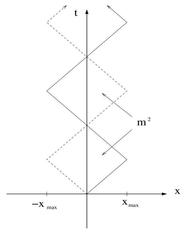
Let $x_{0}=t_{0}=0$, the equation of motion $|x|=t$ is obtained. The maximum kinetic energy at $x=0$ puts an upper bound on the displacement of the particle such that $\kappa x_{max}=W$. The path of the particle is illustrated in Figure 5. The zig-zag motion of the particle is the reason for the name “yoyo state.” The quark-antiquark pair of a meson are assumed to be massless. The mass square of the meson is proportional to the area of the rectangle defined by the trajectories of the quark-antiquark pair. The period $\tau$ of the yoyo motion is [1]

$$\tau={2E_{0}\over\kappa},$$ (30)

where $E_{0}$ is the maximum kinetic energy of each quark. In a boosted Lorentz frame, the period is transformed as [1]

$$\tau^{\prime}=\tau\cosh y.$$ (31)

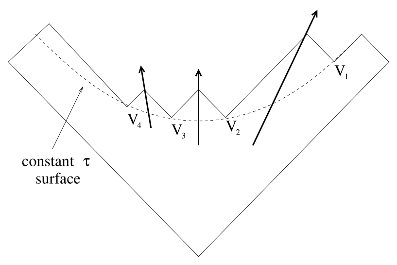
The breakup of a string occurs along a curve of constant proper time such that the process is Lorentz invariant. The Lund model assumes that the produced mesons are ranked, meaning that the production of the $n$-th rank meson depends on the existence of rank $n-1,\,n-2,\,\dots\,,1$ mesons. A vertex $V$ is a breakup point and the location $\kappa(x_{+},x_{-})$ where a quark-antiquark pair is produced. The breakup of a string is represented in Figure 6. The produced particles closer to the edges are the faster moving ones, corresponding to larger rapidities.

Let $p_{\pm 0}$ and $p_{\pm j}$ be momentum of the parent quark and the $j$-th of the $n$ produced quarks moving along the $x_{\pm}$ light-cone coordinate respectively. Then [1]

$$p_{\pm 0}=\sum^{n}_{j=1}p_{\pm j},$$ (32)

and the momentum fraction at $V_{j}$ is defined as [1]

$$z_{\pm j}={p_{\pm j}\over p_{\pm 0}}.$$ (33)

In order to simplify notations, $z_{j}=z_{+j}$ unless specified otherwise. The invariant interval is

$$ds^{2}=dt^{2}-dx^{2}=dt^{2}(1-v^{2}),$$ (34)

giving

$$ds=dt\sqrt{1-v^{2}}={dt\over\gamma}=d\tau,$$ (35)

where $\tau$ is the proper time. The proper time is also $x_{+}x_{-}=(t-x)(t+x)=t^{2}-x^{2}=\tau^{2}$ and can be used as dynamic variable such that [1]

$$\Gamma=\kappa^{2}x_{+}x_{-}.$$ (36)

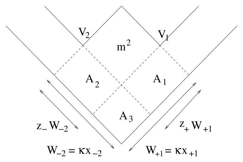
Since $\Gamma$ is proportional to the proper time square $\tau^{2}$, its Lorentz invariant property makes it a good kinematic variable in the light-cone coordinates. Let $W_{\pm 1}$ and $W_{\pm 2}$ be the kinetic energies along $x_{\pm}$ at vertices 1 and 2 respectively. The following identities can be easily proven geometrically by calculating the areas of the rectangles $\Gamma_{1}=A_{1}+A_{3}$, $\Gamma_{2}=A_{2}+A_{3}$ and $m^{2}$ as shown in Figure 7 [1],

$$\Gamma_{1} = (1-z_{-})W_{-2}W_{+1},$$ (37)

$$\Gamma_{2} = (1-z_{+})W_{-2}W_{+1},$$ (38)

$$m^{2} = z_{-}z_{+}W_{-2}W_{+1},$$ (39)

where $m$ is the mass of the produced meson. Eqs. (37) and (38) can be expressed with the help of Eq. (39) as [1]

$$\Gamma_{1} = {m^{2}(1-z_{-})\over z_{+}z_{-}},$$ (40)

$$\Gamma_{2} = {m^{2}(1-z_{+})\over z_{+}z_{-}}.$$ (41)

Differentiating these equations gives [1]

$${\partial\Gamma_{1}\over\partial z_{-}}=-{m^{2}\over z_{+}z_{-}^{2}},$$ (42)

$${\partial\Gamma_{2}\over\partial z_{+}}=-{m^{2}\over z_{+}^{2}z_{-}},$$ (43)

which will be used later in the next section.

Let $H(\Gamma_{1})$ be a probability distribution such that $H(\Gamma_{1})\,d\Gamma_{1}\,dy_{1}$ is the probability of a quark-antiquark pair being produced at the spacetime position $V_{1}$. From now on, the symbol $V_{n}$ also represents the breakup event that leads to the creation of the $n$-th quark-antiquark pair along a surface of constant $\tau$. Let $f(z_{+})dz_{+}$ be the transition probability of obtaining $V_{2}$ given that $V_{1}$ occurs. The transition probability of $V_{2}$ via $V_{1}$ is then $H(\Gamma_{1})\,d\Gamma_{1}\,dy_{1}\,f(z_{+})dz_{+}$. Similarly the probability of $V_{1}$ via $V_{2}$ is $H(\Gamma_{2})\,d\Gamma_{2}\,dy_{2}\,f(z_{-})dz_{-}$. It is reasonable to assume that the probability of $V_{1}$ via $V_{2}$ is equal to that of $V_{2}$ via $V_{1}$ such that [1]

$$H(\Gamma_{1})\,d\Gamma_{1}\,dy_{1}\,f(z_{+})dz_{+}=H(\Gamma_{2})\,d\Gamma_{2}\,dy_{2}\,f(z_{-})dz_{-}.$$ (44)

The Jacobian $J$ in

$$d\Gamma_{1}\,dz_{+}=J\,d\Gamma_{2}\,dz_{-},$$ (45)

is

$$J=\left\Arrowvert\begin{array}[]{cc}{\partial\Gamma_{1}\over\partial\Gamma_{2}}&{\partial\Gamma_{1}\over\partial z_{-}}\\ {\partial z_{+}\over\partial\Gamma_{2}}&{\partial z_{+}\over\partial z_{-}}\end{array}\right\Arrowvert={z_{+}\over z_{-}},$$ (46)

which can be easily computed by using Eqs. (42), (43) and $\partial\Gamma_{1}/\partial\Gamma_{2}=\partial z_{+}/\partial z_{-}=0$. Eq. (45) can now be re-expressed as [1]

$$d\Gamma_{1}{dz_{+}\over z_{+}}=d\Gamma_{2}{dz_{-}\over z_{-}}.$$ (47)

Since rapidity is additive (i. e. $y_{2}=y_{1}+\Delta y$),

$$dy_{1}=dy_{2}.$$ (48)

With Eqs. (47) and (48), Eq. (44) is simplified as [1]

$$H(\Gamma_{1})z_{+}f(z_{+})=H(\Gamma_{2})z_{-}f(z_{-}).$$ (49)

New definitions are now made to facilitate the solution of the equation [1],

$$h(\Gamma) = \log H(\Gamma),$$ (50)

$$g(z) = \log(zf(z)).$$ (51)

The new definitions transform Eq. (49) as [1]

$$h(\Gamma_{1})+g(z_{+})=h(\Gamma_{2})+g(z_{-}).$$ (52)

Notice that [1]

$${\partial^{2}g(z_{+})\over\partial z_{+}\partial z_{-}}={\partial^{2}g(z_{-})\over\partial z_{+}\partial z_{-}}=0.$$ (53)

Differentiate Eq. (52) with respect to $z_{+}$ and $z_{-}$, eliminate terms with $\partial^{2}g/\partial z_{+}\partial z_{-}$ using Eq. (53) and cancel out factors of $\partial\Gamma/\partial z$ on the both sides of the equation to obtain [1]

$${\partial h(\Gamma_{1})\over\partial\Gamma_{1}}+\Gamma_{1}{\partial^{2}h(\Gamma_{1})\over\partial\Gamma_{1}^{2}}={\partial h(\Gamma_{2})\over\partial\Gamma_{2}}+\Gamma_{2}{\partial^{2}h(\Gamma_{2})\over\partial\Gamma_{2}^{2}},$$ (54)

or equivalently [1]

$${d\over d\Gamma}\left(\Gamma\,{dh\over d\Gamma}\right)=-b,$$ (55)

where $b$ is a constant. The solution is [1]

$$h(\Gamma)=-b\Gamma+a\ln\Gamma+\ln C,$$ (56)

where $C$ is a constant of integration. It yields the distribution [1]

$$H(\Gamma)=e^{h(\Gamma)}=C\,\Gamma^{a}\,e^{-b\Gamma}.$$ (57)

Substituting Eqs. (40) and (41) into Eq. (52) gives [1]

$$g_{12}(z_{+})+{bm^{2}\over z_{+}}+a_{1}\ln{m^{2}\over z_{+}}-a_{2}\ln{1-z_{+}\over z_{+}}+\ln C_{1}$$

$$\qquad=g_{21}(z_{-})+{bm^{2}\over z_{-}}+a_{2}\ln{m^{2}\over z_{-}}-a_{1}\ln{1-z_{-}\over z_{-}}+\ln C_{2},$$ (58)

where $g_{12}(z_{+})$ is $g(z_{+})$ of $V_{1}$ transitioning to $V_{2}$ and $g_{21}(z_{-})$ is $g(z_{-})$ of $V_{2}$ transitioning to $V_{1}$. If $a=a_{1}=a_{2}$, the transition probability distribution is [1]

$$f(z_{j})=N\,{1\over z_{j}}\,(1-z_{j})^{a}\,e^{-{bm^{2}\over z_{j}}},$$ (59)

where $N$ is a constant of integration. Otherwise, the transition probability from $V_{\alpha}$ to $V_{\beta}$ is [1]

$$f_{\alpha\beta}(z_{j})=N_{\alpha\beta}\,{1\over z_{j}}\,z_{j}^{a_{\alpha}}\,\left({1-z_{j}\over z_{j}}\right)^{a_{\beta}}e^{-{bm^{2}\over z_{j}}},$$ (60)

where $N_{\alpha\beta}$ is a constant of integration specific to the vertices $V_{\alpha}$ and $V_{\beta}$. Let $z_{0j}$ be the $j$-th rank momentum fraction scaled with respect to $p_{+0}$, then [1]

$$z_{01} = z_{1},$$ (61)

$$z_{02} = z_{2}(1-z_{1}).$$ (62)

The probability of two dependent events is the product of the probabilities of the two individual events. The existence of the rank-2 hadron depends on that of the rank-1 hadron according to the Lund Model so that joint probability of their mutual existence is the product of the two individual probabilities of $V_{1}$ and $V_{2}$. With Eqs. (60-62), the combined distribution of the 1$st$ and 2$nd$ rank hadrons is [1]

$$f(z_{1})dz_{1}\,f(z_{2})dz_{2} = f(z_{01})dz_{01}\,f\left({z_{02}\over 1-z_{01}}\right){dz_{02}\over 1-z_{01}}$$ (63)

$$= {N\,dz_{01}\over z_{01}}\,{N\,dz_{02}\over z_{02}}(1-z_{01})^{a}\left(1-{z_{02}\over 1-z_{01}}\right)^{a}e^{-{bm^{2}\over z_{1}}-{bm^{2}\over z_{2}}}$$

$$= {N\,dz_{01}\over z_{01}}\,{N\,dz_{02}\over z_{02}}(1-z_{01}-z_{02})^{a}\,e^{-b(A_{1}+A_{2})}.$$

The geometical identity $A_{j}=bm^{2}/z_{j}$ is used in the last step. Generalizing the product of two vertices to that of $n$ vertices, the differential probability for the production of $n$ particles is easily seen as [1]

$$dP(1,\dots,n)=(1-z)^{a}\prod^{n}_{j=1}{N\,dz_{0j}\over z_{0j}}\,e^{-bA_{j}},$$ (64)

where $z=\sum^{n}_{j=1}z_{0j}$. Let $p_{0j}=z_{0j}\,p_{+0}$ and $d^{2}p=dp_{+}\,dp_{-}$. Use the identity [1]

$$\int dC\,dB\,\delta(BC-D)={dB\over B}$$ (65)

to obtain [1]

$${dz_{01}\over z_{01}}\,{dz_{02}\over z_{02}}=d^{2}p_{01}\,d^{2}p_{02}\delta^{+}(p_{01}^{2}-m^{2})\,\delta^{+}(p_{01}^{2}-m^{2}).$$ (66)

With Eq. (66), Eq. (64) can be rewritten as [1]

$$dP(p_{01},\dots,p_{0n})=(1-z)^{a}\prod^{n}_{j=1}N\,d^{2}p_{0j}\,\delta^{+}(p_{0j}^{2}-m^{2})\,e^{-bA_{j}}.$$ (67)

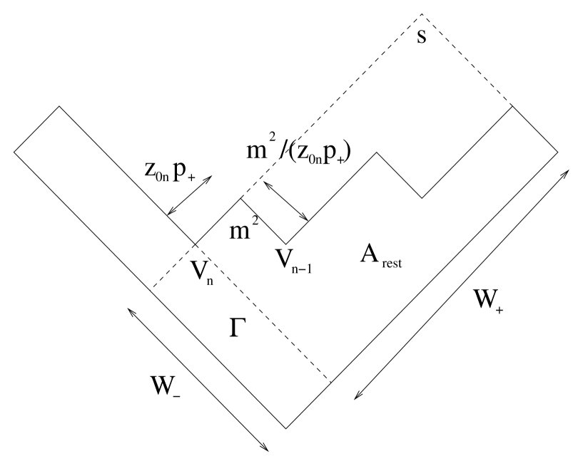
It can be shown from simple geometry in Figure 8 that the kinetic energies of the quarks along the $\pm$ light-cones are [1]

$$W_{+} = z\,p_{0+},$$ (68)

$$W_{-} = \sum^{n}_{j=1}{m_{j}^{2}\over z_{0j}p_{0+}},$$ (69)

and the total kinetic energy square at $V_{n}$ is [1]

$$s=W_{+}W_{-}=\sum^{n}_{j=1}{m^{2}z\over z_{0j}}.$$ (70)

The total differential probability of $n$-particle production is [1]

$$dP(z,s;p_{01},\dots,p_{0n})$$ (71)

$$= dz\,\delta\left(z-\sum^{n}_{j=1}z_{0j}\right)\,ds\,\delta\left(s-\sum^{n}_{j=1}{m^{2}z\over z_{0j}}\right)\,dP(p_{01},\dots,p_{0n})$$

$$= {dz\over z}\,\delta\left(1-\sum^{n}_{j=1}u_{j}\right)\,ds\,\delta\left(s-\sum^{n}_{j=1}{m^{2}\over u_{j}}\right)\,dP(p_{01},\dots,p_{0n}),$$

where $u_{j}\equiv p_{0+j}/W_{n+}$. Use the trick [1]

$$\delta\left(1-\sum^{n}_{j=1}{z_{0j}\over z}\right)\,\delta\left(s-\sum^{n}_{j=1}{m^{2}\over u_{j}}\right)$$ (72)

$$= \delta\left(W_{n+}-W_{n+}\sum^{n}_{j=1}u_{j}\right)\,\delta\left(W_{n-}-\sum^{n}_{j=1}{m^{2}\over u_{j}W_{n+}}\right)$$

$$= \delta\left(W_{n+}-\sum^{n}_{j=1}p_{0j+}\right)\,\delta\left(W_{n-}-\sum^{n}_{j=1}p_{0j-}\right)$$

$$\equiv \delta^{2}\left(p_{rest}-\sum^{n}_{j=1}p_{0j}\right),$$

where $p_{rest}=(W_{n+},W_{n-})$, to re-organize Eq. (71) as [1]

$$dP(z,s;p_{01},\dots,p_{0n}) = ds\,{dz\over z}\,(1-z)^{a}\,e^{-b\Gamma}\delta\left(p_{rest}-\sum^{n}_{j=1}p_{0j}\right)$$ (73)

$$\quad\times\prod^{n}_{j=1}N\,d^{2}p_{0j}\,\delta^{+}(p_{0j}^{2}-m^{2})\,e^{-bA_{rest}},$$

with the definition [1]

$$A_{total}\equiv\sum^{n}_{j=1}A_{j}=\Gamma+A_{rest}.$$ (74)

The claim is that $A_{total}$ is Lorentz invariant. It is called the “Area Law” [7]. Eq. (73) can be separated in the external and internal parts as in [1]

$$dP_{ext} = ds\,{dz\over z}\,(1-z)^{a}\,e^{-b\Gamma},$$ (75)

$$dP_{int} = \prod^{n}_{j=1}N\,d^{2}p_{0j}\,\delta^{+}(p_{0j}^{2}-m^{2})\,\delta\left(p_{rest}-\sum^{n}_{j=1}p_{0j}\right)\,e^{-bA_{rest}}.$$ (76)

The external part contains kinematic variables $s$, $z$ and $\Gamma$. The internal part contains dynamic variables $p_{0j}$. Eqs. (75) and (76) are the final results.

3 The Parton Model

The relevant formulas of the parton model in reference [2] are derived below. Several mistakes found in reference [2] have been corrected here.

3.1 External Cross Section Formulas

The Feynman diagram of hadrons $A$ and $B$ scattering into partons $c$ and $d$, $A+B\to c+d$, is illustrated in Figure 9. The external Mandelstam variables are defined as

$$s \equiv (P_{A}+P_{B})^{2}=2P_{A}\cdot P_{B},$$ (77)

$$t \equiv (p_{c}-P_{A})^{2}=-2p_{c}\cdot P_{A}=-{s\over 2}\,x_{T}\,{\mathcal{T}}_{c},$$ (78)

$$u \equiv (p_{c}-P_{B})^{2}=-2p_{c}\cdot P_{B}=-{s\over 2}\,x_{T}\,{1\over{\mathcal{T}}_{c}},$$ (79)

where

$$x_{T}\equiv{2\,p_{T}\over\sqrt{s}},$$ (80)

and

$${\mathcal{T}}_{c}\equiv\tan{\theta_{c}\over 2}.$$ (81)

Eq. (78) is proved as follow: In the high energy limit, $m_{i}=0,\,\forall i,$ such that $E_{i}=|{\mathbf{p}}_{i}|$.

$$E_{A}=E_{B}=|{\mathbf{P}}_{A}|=|{\mathbf{P}}_{B}|={\sqrt{s}\over 2}.$$ (82)

From Figure 9, it is obvious that

$$p_{T}=|\mathbf{p}_{c}|\sin\theta_{c}.$$ (83)

$$t = -2\,p_{c}\cdot P_{A}$$ (84)

$$= -2\,(E_{c}E_{A}-|{\mathbf{p}}_{c}||{\mathbf{P}}_{A}|\cos\theta_{c})$$ (85)

$$= -2\,(|{\mathbf{p}}_{c}||{\mathbf{P}}_{A}|-|{\mathbf{p}}_{c}||{\mathbf{P}}_{A}|\cos\theta_{c})$$ (86)

$$= -2\,p_{T}\,|\mathbf{P}_{A}|\,{1-\cos\theta_{c}\over\sin\theta_{c}}$$ (87)

$$= -2\,\left({x_{T}\sqrt{s}\over 2}\right)\left({\sqrt{s}\over 2}\right){1-(1-2\sin^{2}(\theta_{c}/2))\over 2\sin(\theta_{c}/2)\cos(\theta_{c}/2)}$$ (88)

$$= -{s\over 2}\,x_{T}\,{\mathcal{T}}_{c}.$$ (89)

Similarly,

$$u = -2\,p_{c}\cdot P_{B}$$ (90)

$$= -2\,(E_{c}E_{B}-|\mathbf{p}_{c}||\mathbf{P}_{B}|\cos(180^{\circ}-\theta_{c}))$$ (91)

$$= -2\,(E_{c}E_{B}+|\mathbf{p}_{c}||\mathbf{P}_{B}|\cos\theta_{c})$$ (92)

$$= -{s\over 2}\,x_{T}\,{1\over{\mathcal{T}}_{c}}.$$ (93)

In the massless limit, the sum rule of external Mandelstam variables is

$$s+t+u=0.$$ (94)

A fraction, $x_{i}$, of the momentum of the incoming hadron $P_{i}$ makes up the momentum of parton $p_{i}$. More specifically, we have

$$p_{a} = x_{a}\,P_{A},$$ (95)

$$p_{b} = x_{b}\,P_{B}.$$ (96)

These imply that

$$|\mathbf{p}_{a}| = {x_{a}\sqrt{s}\over 2},$$ (97)

$$|\mathbf{p}_{b}| = {x_{b}\sqrt{s}\over 2}.$$ (98)

The internal Mandelstam variables, $\hat{s}$, $\hat{t}$ and $\hat{u}$, of the partons can now be written in terms of the external Mandelstam variables, $s$, $t$ and $u$.

$$\hat{s} = (p_{a}+p_{b})^{2}=2p_{a}\cdot p_{b}=x_{a}x_{b}s,$$ (99)

$$\hat{t} = (p_{c}-p_{a})^{2}=-2p_{c}\cdot p_{a}=x_{a}t,$$ (100)

$$\hat{u} = (p_{c}-p_{b})^{2}=-2p_{c}\cdot p_{b}=x_{b}u.$$ (101)

The conservation of energy-momentum is given as

$$p_{a}+p_{b}=p_{c}+p_{d}.$$ (102)

From the expressions of the internal and external Mandelstam variables, it is easily seen that

$$p_{T}^{2}={tu\over s}={\hat{t}\hat{u}\over\hat{s}}.$$ (103)

In the massless limit, the sum rule of the internal Mendalstam variables is

$$\hat{s}+\hat{t}+\hat{u}=0,$$ (104)

or equivalently,

$$x_{a}x_{b}s+x_{a}t+x_{b}u=0$$ (105)

From Eq. (105), we have

$$x_{a}={-x_{b}u\over x_{b}s+t}={-x_{b}u/s\over x_{b}+t/s}={x_{b}x_{1}\over x_{b}-x_{2}},$$ (106)

where

$$x_{1} \equiv -{u\over s}={1\over 2}\,x_{T}\,{1\over{\mathcal{T}}_{c}},$$ (107)

$$x_{2} \equiv -{t\over s}={1\over 2}\,x_{T}\,{\mathcal{T}}_{c}.$$ (108)

Similarly,

$$x_{b}={-x_{a}t\over x_{a}s+u}={-x_{a}t/s\over x_{a}+u/s}={x_{a}x_{2}\over x_{a}-x_{1}},$$ (109)

The expression $\hat{t}=(p_{c}-p_{a})^{2}=(p_{d}-p_{b})^{2}$ can be considered separately as

$$\hat{t} = (p_{c}-p_{a})^{2}=-2p_{c}\cdot p_{a}=-{s\over 2}\,x_{T}\,x_{a}\,{\mathcal{T}}_{c},$$ (110)

$$\hat{t} = (p_{d}-p_{b})^{2}=-2p_{d}\cdot p_{b}=-{s\over 2}\,x_{T}\,x_{b}\,{1\over{\mathcal{T}}_{d}},$$ (111)

where

$${\mathcal{T}}_{d}\equiv\tan{\theta_{d}\over 2}.$$ (112)

Eqs. (110) and (111) imply that

$$x_{a}\,{\mathcal{T}}_{c}=x_{b}\,{1\over{\mathcal{T}}_{d}}.$$ (113)

The internal Mandelstam variables can be re-expressed in terms of the external angles as follow.

$$|\mathbf{p}_{a}-\mathbf{p}_{b}| = |\mathbf{p}_{c}|\cos\theta_{c}+|\mathbf{p}_{d}|\cos\theta_{d}$$ (114)

$$= {p_{T}\over\sin\theta_{c}}\,\cos\theta_{c}+{p_{T}\over\sin\theta_{d}}\,\cos\theta_{d},$$ (115)

which implies

$$|x_{a}\,\mathbf{P}_{A}-x_{b}\,\mathbf{P}_{B}| = \left|x_{a}\,{\sqrt{s}\over 2}-x_{b}\,{\sqrt{s}\over 2}\right|$$ (116)

$$= p_{T}(\cot\theta_{c}+\cot\theta_{d}),$$ (117)

or equivalently

$$x_{a}-x_{b} = x_{T}\,(\cot\theta_{c}+\cot\theta_{d})$$ (118)

$$= x_{T}\,\left({1-\tan^{2}(\theta_{c}/2)\over 2\tan(\theta_{c}/2)}+{1-\tan^{2}(\theta_{d}/2)\over 2\tan(\theta_{d}/2)}\right)$$ (119)

$$= x_{T}\,\left({1-{\mathcal{T}}_{c}^{2}\over 2{\mathcal{T}}_{c}}+{1-{\mathcal{T}}_{d}^{2}\over 2{\mathcal{T}}_{d}}\right)$$ (120)

$$= {1\over 2}\,x_{T}\,\left[\left({1\over{\mathcal{T}}_{c}}-{\mathcal{T}}_{c}\right)+\left({1\over{\mathcal{T}}_{d}}-{\mathcal{T}}_{d}\right)\right].$$ (121)

Eqs. (113) and (121) together give

$$x_{a} = {1\over 2}\,x_{T}\,\left({1\over{\mathcal{T}}_{c}}+{1\over{\mathcal{T}}_{d}}\right),$$ (122)

$$x_{b} = {1\over 2}\,x_{T}\,\left({\mathcal{T}}_{c}+{\mathcal{T}}_{d}\right).$$ (123)

Finally, the internal Mendalstam variables can be re-expressed in terms of the external angles as

$$\hat{s} = {s\over 4}\,x_{T}^{2}\,\left(2+{{\mathcal{T}}_{c}\over{\mathcal{T}}_{d}}+{{\mathcal{T}}_{d}\over{\mathcal{T}}_{c}}\right),$$ (124)

$$\hat{t} = {s\over 4}\,x_{T}^{2}\,\left(1+{{\mathcal{T}}_{c}\over{\mathcal{T}}_{d}}\right),$$ (125)

$$\hat{u} = {s\over 4}\,x_{T}^{2}\,\left(1+{{\mathcal{T}}_{d}\over{\mathcal{T}}_{c}}\right).$$ (126)

Eqs. (124)–(126) will not be used directly in this work. However it is interesting to know that the internal Mendalstam variables can be measured in terms of the external angles. Another interesting fact worth mentioning is that Eqs. (106) and (109) are still true even if ${\mathcal{T}}_{c}$ is replaced by ${\mathcal{T}}_{d}$ in Eqs. (107) and (108). This statement can be checked easily by substituting Eq. (113) into Eqs. (106) and (109) and then solving for $x_{a}$ and $x_{b}$. The interchangability of ${\mathcal{T}}_{c}$ and ${\mathcal{T}}_{d}$ will become useful later in some of the derivations below.

The differential cross section of parton production for the reaction $A+B\to c+d$ is

$$d\sigma=f_{A/a}(x_{a},Q^{2})dx_{a}\,f_{B/b}(x_{b},Q^{2})dx_{b}\,{d\hat{\sigma}\over d\hat{t}}\,d\hat{t},$$ (127)

where $f_{A/a}(x_{a},Q^{2})$ and $f_{B/b}(x_{b},Q^{2})$ are the renormalized parton distribution functions (PDF’s) of parton $a$ in hadron $A$ and of parton $b$ in hadron $B$ respectively. Although $Q^{2}$ has a simple interpretation in QED,

$$Q^{2}=(p^{\prime}-p)^{2}={1\over 2}\,E^{\prime}E\sin{\theta\over 2}$$ (128)

(where $p$ and $p^{\prime}$ are the incoming and outgoing lepton momenta and $\theta$ is the scattering angle), there is no clear understanding of what is $Q^{2}$ in hadron collisions. Some good guesses are

$$Q^{2} = 4\hat{p}^{2}_{T},$$ (129)

$$Q^{2} = {2\hat{s}\hat{t}\hat{u}\over\hat{s}^{2}+\hat{t}^{2}+\hat{u}^{2}}.$$ (130)

Although the interest of this work is not parton production per se, it serves as an intuitive starting point to introduce hadron production later.

The substitution of Eqs. (107) and (108) into Eq. (106) gives

$$x_{a}x_{b}-{1\over 2}\,x_{a}x_{T}{\mathcal{T}}_{c}={1\over 2}\,x_{b}x_{T}\,{1\over{\mathcal{T}}_{c}}.$$ (131)

Differentiating $x_{b}$ in Eq. (131) with respect to ${\mathcal{T}}_{c}$ and $x_{T}$ while keeping $x_{a}$ fixed gives

$${\partial x_{b}\over\partial{\mathcal{T}}_{c}} = {x_{a}x_{T}{\mathcal{T}}_{c}-x_{b}x_{T}\,{\mathcal{T}}_{c}^{-1}\over 2x_{a}{\mathcal{T}}_{c}-x_{T}},$$ (132)

$${\partial x_{b}\over\partial x_{T}} = {x_{b}+x_{a}{\mathcal{T}}_{c}^{2}\over 2x_{a}{\mathcal{T}}_{c}-x_{T}}.$$ (133)

Repeating the same process with $\hat{t}=-{s\over 2}\,x_{T}x_{a}{\mathcal{T}}_{c}$ yields

$${\partial\hat{t}\over\partial{\mathcal{T}}_{c}} = -{s\over 2}\,x_{T}x_{a},$$ (134)

$${\partial\hat{t}\over\partial x_{T}} = -{s\over 2}\,x_{a}{\mathcal{T}}_{c}.$$ (135)

The Jacobian now can be computed with Eqs. (132)–(135) as

$${\partial(x_{b},\hat{t})\over\partial({\mathcal{T}}_{c},x_{T})}={x_{a}\,x_{b}\,x_{T}\,s\over 2x_{a}{\mathcal{T}}_{c}-x_{T}}={x_{a}\,x_{b}\,x_{T}\,s\over 2(x_{a}-x_{1}){\mathcal{T}}_{c}}.$$ (136)

or

$${\partial(x_{b},\hat{t})\over\partial(\theta_{c},x_{T})} = {\partial(x_{b},\hat{t})\over\partial({\mathcal{T}}_{c},x_{T})}\,{d{\mathcal{T}}_{c}\over d\theta_{c}}$$ (137)

$$= {x_{a}\,x_{b}\,x_{T}\,s\over 2(x_{a}-x_{1}){\mathcal{T}}_{c}}\left({1-{\mathcal{T}}_{c}^{2}\over 2}\right)$$ (138)

$$= {s\over 2}\,{x_{a}x_{b}\over x_{a}-x_{1}}\,{x_{T}\over\sin\theta_{c}}$$ (139)

Given that $E=m_{T}\cosh y$ and $p_{z}=m_{T}\sinh y$, $dp_{z}/dy=E$. In the cylindrical coordinates,

$$dp^{3} = \pi dp_{z}\,dp_{T}^{2}$$ (140)

$$= \pi Edy\,dp_{T}^{2}.$$ (141)

With $p_{T}^{2}={s\over 2}\,x_{T}\,dx_{T}$,

$$dp_{T}^{2}={s\over 2}\,x_{T}\,dx_{T}.$$ (142)

And with

$$y={1\over 2}\,\ln{1+\cos\theta_{c}\over 1-\cos\theta_{c}},$$ (143)

there is also

$$dy={d\theta_{c}\over\sin\theta_{c}}.$$ (144)

Substitute Eqs. (142) and (144) into Eq. (141) to get

$${dp^{3}\over E} = \pi\,dy\,dp_{T}^{2}$$ (145)

$$= {\pi\over 2}\,{x_{T}\,s\over\sin\theta_{c}}\,d\theta_{c}\,dx_{T}.$$ (146)

Combine the Jacobian in Eq. (139) with Eq. (146) and obtain

$$dx_{b}\,d\hat{t}={1\over\pi}\,{x_{a}x_{b}\over x_{a}-x_{1}}\,{dp^{3}\over E}.$$ (147)

With Eq. (147), the Lorentz invariant differential parton production cross section from Eq. (127) can be written as

$$E{d^{3}\sigma\over dp^{3}}={1\over\pi}\,f_{A/a}(x_{a},Q^{2})dx_{a}\,f_{B/b}(x_{b},Q^{2})\,{x_{a}x_{b}\over x_{a}-x_{1}}\,{d\hat{\sigma}\over d\hat{t}}.$$ (148)

The inclusive cross section for $A+B\to c+X$ can be obtained from Eq. (148) by integrating over $\theta_{d}$, or equivalently by integrating over $x_{a}$ as in $dx_{a}=(x_{a}-x_{1})\,dy_{d}$. The relationship between $dy_{d}$ and $dx_{a}$ can be derived as follow. Substitute Eqs. (113), (107) and (108) into Eq. (109) and obtain

$$x_{a}{\mathcal{T}}_{c}\,{\mathcal{T}}_{d}={x_{a}\left({1\over 2}\,x_{T}{\mathcal{T}}_{d}\right)\over x_{a}-{1\over 2}\,x_{T}{\mathcal{T}}_{d}}.$$ (149)

$x_{a}$ can be isolated from Eq. (149) as

$$x_{a}-{1\over 2}\,x_{T}\,{1\over{\mathcal{T}}_{d}}=x_{1}.$$ (150)

Differentiating Eq. (150) with $x_{T}$ and $x_{1}$ held fixed yields

$$dx_{a} = {1\over 2}\,x_{T}\,{1\over{\mathcal{T}}_{d}^{2}}\,d{\mathcal{T}}_{d}$$ (151)

$$= {1\over 2}\,x_{T}\,{1\over{\mathcal{T}}_{d}}\,dy_{d}$$ (152)

$$= {1\over 2}\,x_{T}\,{x_{a}{\mathcal{T}}_{c}\over x_{b}}\,dy_{d}$$ (153)

$$= {x_{a}x_{2}\over x_{b}}\,dy_{d}$$ (154)

$$= (x_{a}-x_{1})\,dy_{d}.$$ (155)

The inclusive cross section for $A+B\to c+X$ is

$$E{d^{3}\sigma\over dp^{3}}={1\over\pi}\int^{1}_{x_{a}^{min}}dx_{a}\,f_{A/a}(x_{a},Q^{2})\,f_{B/b}(x_{b},Q^{2})\,{x_{a}x_{b}\over x_{a}-x_{1}}\,{d\hat{\sigma}\over d\hat{t}},$$ (156)

where

$$x_{a}^{min}={x_{1}\over 1-x_{2}}={x_{T}/{\mathcal{T}}_{c}\over 2-x_{T}{\mathcal{T}}_{c}}.$$ (157)

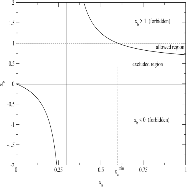
The lower limit of the integral in Eq. (156) is not zero is that $x_{a}$, as seen in Eq. (106). $x_{a}<0$ for $x_{b}<x_{2}$, which is not allowed. At $x_{b}=x_{2}$, $x_{a}\to\infty$, which is also impossible. Hence the value of $x_{a}$ is limited by a range of $x_{b}$. It can be seen in Figure 10 that $x_{a}$ is at its minimum when $x_{b}=1$ and the maximum value of $x_{a}$ is 1.

Once the formalism of parton production is complete, the derivation of the inclusive hadron production cross section can be essentially the same. The external Mandelstam variables are similarly defined,

$$s \equiv (P_{A}+P_{B})^{2}=2P_{A}\cdot P_{B},$$ (158)

$$t \equiv (P_{h}-P_{A})^{2}=-2p_{h}\cdot P_{A}=-{s\over 2}\,x_{T}{\mathcal{T}}_{h},$$ (159)

$$u \equiv (P_{h}-P_{B})^{2}=-2p_{h}\cdot P_{B}=-{s\over 2}\,x_{T}\,{1\over{\mathcal{T}}_{h}}.$$ (160)

The internal Mandelstam variables are slightly modified as

$$\hat{s} \equiv (p_{a}+p_{b})^{2}=x_{a}x_{b}s,$$ (161)

$$\hat{t} \equiv (p_{c}-p_{a})^{2}=-2p_{c}\cdot p_{a}=-2{P_{h}\over z_{c}}\cdot p_{a}={x_{a}t\over z_{c}},$$ (162)

$$\hat{u} \equiv (p_{c}-p_{b})^{2}=-2p_{c}\cdot p_{b}=-2{P_{h}\over z_{c}}\cdot p_{b}={x_{b}u\over z_{c}},$$ (163)

where

$$p_{a} = x_{a}P_{A},$$ (164)

$$p_{b} = x_{b}P_{B},$$ (165)

$$P_{h} = z_{c}p_{c}.$$ (166)

Eq. (104) combined with Eqs. (161)–(166) gives

$$z_{c}={x_{2}\over x_{b}}+{x_{1}\over x_{a}},$$ (167)

with

$$x_{1} = -{u\over s}={1\over 2}\,x_{T}\,{1\over{\mathcal{T}}_{h}},$$ (168)

$$x_{2} = -{t\over s}={1\over 2}\,x_{T}\,{\mathcal{T}}_{h},$$ (169)

$${\mathcal{T}}_{h} = \tan{\theta_{cm}\over 2}.$$ (170)

Differentiate Eq. (167) to obtain

$${\partial z_{c}\over\partial\theta_{cm}} = {1\over 4}\,\left(-{1\over x_{a}{\mathcal{T}}_{h}^{2}}+{{\mathcal{T}}_{h}\over x_{b}}\right)\,\sec^{2}{\theta_{cm}\over 2},$$ (171)

$${\partial z_{c}\over\partial x_{T}} = {1\over 2}\,\left({1\over x_{a}{\mathcal{T}}_{h}}+{{\mathcal{T}}_{h}\over x_{b}}\right),$$ (172)

$${\partial\hat{t}\over\partial\theta} = -{1\over 4}\,{x_{T}x_{a}\over z_{c}}\,\sec^{2}{\theta_{cm}\over 2},$$ (173)

$${\partial\hat{t}\over\partial x_{T}} = -{1\over 2}\,{x_{a}\over z_{c}}\,{\mathcal{T}}_{h}.$$ (174)

The Jacobian can be computed from Eqs. (171)–(174),

$${\partial(z_{c},\hat{t})\over\partial(\theta_{cm},x_{T})}={x_{T}\,s\over 2z_{c}\sin\theta_{cm}}.$$ (175)

As before,

$$d\theta_{cm}\,dx_{T}={2\over\pi s}\,{\sin\theta_{cm}\over x_{T}}\,{dp^{3}\over E},$$ (176)

such that

$$dz_{c}\,d\hat{t}={1\over\pi z_{c}}\,{dp^{3}\over E}.$$ (177)

The differential hadron production cross section is

$$d\sigma=f_{A/a}(x_{a},Q^{2})dx_{a}\,f_{B/b}(x_{b},Q^{2})dx_{b}\,{d\hat{\sigma}\over d\hat{t}}\,d\hat{t}\,D^{h}_{c}(z_{c},Q^{2})dz_{c}.$$ (178)

The major difference between the parton and hadron cross section formulas is the inclusion of the fragmentation function (FF), $D^{h}_{c}(z_{c},Q^{2})$. The inclusive hadron production cross section is

$$E\,{d^{3}\sigma\over dp^{3}}={1\over\pi}\,\int^{1}_{x_{a}^{min}}dx_{a}\int^{1}_{x_{b}^{min}}dx_{b}\,f_{A/a}(x_{a},Q^{2})\,f_{B/b}(x_{b},Q^{2})\,D^{h}_{c}(z_{c},Q^{2})\,{1\over z_{c}}\,{d\hat{\sigma}\over d\hat{t}},$$ (179)

with

$$x_{a}^{min} = {x_{1}\over 1-x_{2}},$$ (180)

$$x_{b}^{min} = {x_{a}x_{2}\over x_{a}-x_{1}}.$$ (181)

3.2 Internal Cross Section Formulas

The internal cross sections,

$${d\hat{\sigma}\over d\hat{t}}(ab\to cd;\hat{s},\hat{t})={\pi\alpha_{s}^{2}(Q^{2})\over\hat{s}^{2}}\,|\overline{\mathcal{M}}(ab\to cd)|^{2},$$ (182)

are derived by adding the leading order Feynman diagrams [13] together, with

$$|\overline{\mathcal{M}}(q_{i}q_{j}\to q_{i}q_{j})|^{2} = |\overline{\mathcal{M}}(q_{i}\overline{q}_{j}\to q_{i}\overline{q}_{j})|^{2}={4\over 9}\,{\hat{s}^{2}+\hat{u}^{2}\over\hat{t}^{2}},$$ (183)

$$|\overline{\mathcal{M}}(q_{i}q_{i}\to q_{i}q_{i})|^{2} = {4\over 9}\,\left({\hat{s}^{2}+\hat{u}^{2}\over\hat{t}^{2}}+{\hat{s}^{2}+\hat{t}^{2}\over\hat{u}^{2}}\right)-{8\over 27}\,{\hat{s}^{2}\over\hat{u}\hat{t}},$$ (184)

$$|\overline{\mathcal{M}}(q_{i}\overline{q}_{i}\to q_{i}\overline{q}_{i})|^{2} = {4\over 9}\,\left({\hat{s}^{2}+\hat{u}^{2}\over\hat{t}^{2}}+{\hat{t}^{2}+\hat{u}^{2}\over\hat{s}^{2}}\right)-{8\over 27}\,{\hat{u}^{2}\over\hat{s}\hat{t}},$$ (185)

$$|\overline{\mathcal{M}}(q_{i}\overline{q}_{i}\to gg)|^{2} = {32\over 27}\,\left({\hat{u}^{2}+\hat{t}^{2}\over\hat{u}\hat{t}}\right)-{8\over 3}\,\left({\hat{u}^{2}+\hat{t}^{2}\over\hat{s}^{2}}\right),$$ (186)

$$|\overline{\mathcal{M}}(gg\to q_{i}\overline{q}_{i})|^{2} = {1\over 6}\,\left({\hat{u}^{2}+\hat{t}^{2}\over\hat{u}\hat{t}}\right)-{3\over 8}\,\left({\hat{u}^{2}+\hat{t}^{2}\over\hat{s}^{2}}\right),$$ (187)

$$|\overline{\mathcal{M}}(q_{i}g\to q_{i}g)|^{2} = -{4\over 9}\,\left({\hat{u}^{2}+\hat{s}^{2}\over\hat{u}\hat{s}}\right)+\left({\hat{u}^{2}+\hat{s}^{2}\over\hat{t}^{2}}\right),$$ (188)

$$|\overline{\mathcal{M}}(gg\to gg)|^{2} = {9\over 2}\,\left(3-{\hat{u}\hat{t}\over\hat{s}^{2}}-{\hat{u}\hat{s}\over\hat{t}^{2}}-{\hat{s}\hat{t}\over\hat{u}^{2}}\right),$$ (189)

and

$$\alpha_{LO}(Q^{2})={12\pi\over(33-2n_{f})\log\left({Q^{2}\over\Lambda^{2}}\right)},$$ (190)

$$\alpha_{s}(Q^{2})=\alpha_{LO}(Q^{2})\left[1-{1\over 4\pi}\,{306-38n_{f}\over 33-2n_{f}}\,\alpha_{LO}(Q^{2})\log\log\left({Q^{2}\over\Lambda^{2}}\right)\right],$$ (191)

where $n_{f}$ is the number of flavors and $\Lambda_{\overline{MS}}\approx 0.2\,{\rm GeV}^{2}$ by convention.

3.3 Fragmentation Functions

The fragmentation function, $D^{h}_{q}(z,Q^{2})$, registers the number of hadrons of type $h$ with energy fraction,

$$z={2E_{h}\over Q},$$ (192)

per $dz$ generated by the initial quark $q$. Energy conservation gives

$$\sum_{h}\int^{1}_{0}zD^{h}_{q}(z,Q^{2})\,dz=1.$$ (193)

It is assumed that scaling occurs, i. e.

$$D^{h}_{q}(z,Q^{2})=D^{h}_{q}(z).$$ (194)

The multiplicity of $h$ emerging from $q$ is

$$\int^{1}_{z_{min}}D^{h}_{q}(z)\,dz,$$ (195)

where $z_{min}=2m_{h}/Q$. The fragmentation function cannot be calculated exactly by QCD. Feynman and Field have a semi-analytical parameterization [2], which is now being described below. Let $f(\eta)\,d\eta$ be the probability that the first hierarchy (rank 1) meson leaves fractional momentum $\eta$ to the remaining cascade. The function $f(\eta)$ is normalized,

$$\int^{1}_{0}f(\eta)\,d\eta=1.$$ (196)

Secondly let $F(z)\,dz$ be the probability of finding a meson (independent of rank) with fractional momentum $z$ within $dz$ in a jet. Feynman and Field assumed a simple stochastic ansatz that probability distribution is recursive. This way $F(z)$ satisfies the integral equation

$$F(z)=f(1-z)+\int^{1}_{z}{d\eta\over\eta}\,f(\eta)\,F(z/\eta).$$ (197)

The first term gives the probability that the produced meson is rank 1. The second term calculates the probability of the production of a higher rank meson recursively. Data of deep inelastic scattering experiments suggest the simple form

$$zF(z)=f(1-z)=(n+1)(1-z)^{n}.$$ (198)

The power $n=2$ gives a qualitative description of experimental data.

Next the flavor dependent part of the fragmentation function is considered. Let $\beta_{i}$ be the probability of the $q_{i}\overline{q}_{i}$ pair. The normalization condition imposes that

$$\sum^{n_{f}}_{i=1}\beta_{i}=1.$$ (199)

The isospin symmetry implies that

$$\beta_{u}=\beta_{d}=\beta.$$ (200)

Furthermore, data indicate that $\beta_{s}\approx{1\over 2}\,\beta_{u}$ and that $\beta_{c}$ and $\beta_{b}$ are small. For a quark of flavor $q$, the mean number of meson states of flavor $a\overline{b}$ at $z$ is, in analogy of Eq. (197), given by

$$P^{a\overline{b}}_{q}(z)=\delta_{aq}\beta_{b}f(1-z)+\int^{1}_{z}{d\eta\over\eta}\,f(\eta)\,\beta_{q}\,P^{a\overline{b}}_{q}(z/\eta).$$ (201)

The mean number of meson states averaged over all quarks is

$$P^{a\overline{b}}_{<q>}(z)=\sum_{c}\beta_{c}P^{a\overline{b}}_{c}(z),$$ (202)

so that

$$P^{a\overline{b}}_{<q>}(z)=\beta_{a}\beta_{b}f(1-z)+\int^{1}_{z}{d\eta\over\eta}\,f(\eta)\,P^{a\overline{b}}_{<q>}(z/\eta).$$ (203)

Comparing with Eq. (197) yields

$$P^{a\overline{b}}_{<q>}(z)=\beta_{a}\beta_{b}F(z).$$ (204)

Comparing Eqs. (201), (203) and (204) yields

$$P^{a\overline{b}}_{q}(z)=\delta_{aq}\beta_{b}f(1-z)+\beta_{a}\beta_{b}\overline{F}(z),$$ (205)

where

$$\overline{F}(z)=F(z)-f(1-z).$$ (206)

Eqs. (198) and (206) together give

$$z\overline{F}(z)=(n+1)(1-z)^{n+1}.$$ (207)

The mean number of meson state, $P^{a\overline{b}}_{q}(z)$, is related to the fragmentation function as in

$$D^{h}_{q}(z)=\sum_{a,b}\Gamma^{h}_{a\overline{b}}P^{a\overline{b}}_{q}(z),$$ (208)

where $\Gamma^{h}_{a\overline{b}}$ is the probability of $h$ containing $a\overline{b}$. For example, $\Gamma^{\pi^{+}}_{u\overline{d}}=1$ and $\Gamma^{\pi^{0}}_{u\overline{u}}=\Gamma^{\pi^{0}}_{d\overline{d}}={1\over 2}$. Substitute Eq. (205) into Eq. (208) to obtain

$$D^{h}_{q}(z)=A^{h}_{q}f(1-z)+B^{h}\overline{F}(z),$$ (209)

where

$$A^{h}_{q} = \sum_{b}\Gamma^{h}_{q\overline{b}}\beta_{b},$$ (210)

$$B^{h} = \sum_{q}\beta_{q}A^{h}_{q}.$$ (211)

As a example, given that $\beta_{u}=\beta_{d}=2\beta_{s}=\beta$ and $\beta_{c}=\beta_{b}=\beta_{t}=0$, it is easily shown that $\beta=0.4$, and

$$A^{\pi^{0}}_{u} = {1\over 2}\,\beta,$$ (212)

$$A^{\pi^{0}}_{d} = {1\over 2}\,\beta,$$ (213)

$$A^{\pi^{0}}_{s} = 0,$$ (214)

$$B^{\pi^{0}} = \beta^{2}.$$ (215)

3.4 Implementing the Feynman-Field Model

Feynman and Field calculated the invariant production cross section formula by incorporating the structure functions (or pardon distribution functions), $f_{A/a}(x_{a},Q^{2})$, obtained from DIS experiments and the fragmentation functions, $D^{h}_{q}(z,Q^{2})$, derived from a combination of stochastic arguments and parameterizations of data. The cross section formula

$$E\,{d^{3}\sigma\over dp^{3}}={1\over\pi}\sum_{a,b}\int^{1}_{x_{a}^{min}}dx_{a}\int^{1}_{x_{b}^{min}}dx_{b}\,f_{A/a}(x_{a},Q^{2})\,f_{B/b}(x_{b},Q^{2})\,D^{h}_{c}(z_{c},Q^{2})\,{1\over z_{c}}\,{d\hat{\sigma}\over d\hat{t}},$$ (216)

with

$$x_{a}^{min} = {x_{1}\over 1-x_{2}},$$ (217)

$$x_{b}^{min} = {x_{a}x_{2}\over x_{a}-x_{1}},$$ (218)

is derived explicitly in Appendix 3. The invariant cross section is of interest because it can be used to calculate a number of physical quantities. For instance, the particle number ${\mathcal{N}}_{h}$ of hadron $h$ can be calculated as [8]

$${\mathcal{N}}_{h}={{\mathcal{N}}_{p}(1+K_{h})\over\sigma^{pp}_{in}}\,\int V(r)\,E\,{d^{3}\sigma\over dp^{3}}\,W(p,r)\,{d^{3}p\over E}\,d^{3}r,$$ (219)

where ${\mathcal{N}}_{p}$ is the protons incident on the target; $W(p,r)$ is the probability of recording a pion produced in the target with coordinate $r$ and momentum $p$, $V(r)\,d^{3}r$ is the probability for the incident proton to interact in the element $d^{3}r$ in the target; $K_{h}$ is a coefficient which takes into account the probability of pion production as a result of two or more interactions in the target. Blattnig et al. [11] calculated the spectral distribution and the total cross section from the invariant cross section as in

$${d\sigma\over dE}=2\pi p\int^{\theta_{max}}_{0}d\theta\,E\,{d^{3}\sigma\over dp^{3}}\,\sin\theta,$$ (220)

and

$$\sigma=2\pi\int^{\theta_{max}}_{0}d\theta\int^{p_{max}}_{p_{min}}\,dp\,E\,{d^{3}\sigma\over dp^{3}}\,{p^{2}\sin\theta\over\sqrt{p^{2}+m^{2}_{h}}},$$ (221)

where $m_{h}$ is the mass of the produced hadron. These are just some examples to show why $E\,d^{3}\sigma/dp^{3}$ is an interesting quantity to calculate.

Monte Carlo integration package VEGAS is used to calculate Eq. (216). VEGAS uses a mixed strategy combining importance and stratified sampling. The details of this method can be found in references [3, 9]. Inputs used in VEGAS are given as follow.

$$ndim = 2,$$ (222)

$$ncall = 5000,$$ (223)

$$itmx = 5,$$ (224)

$$nprn = 0,$$ (225)

$$xl[1] = regn[1]={x_{1}\over 1-x_{2}},$$ (226)

$$xl[2] = regn[2]={x_{2}\over 1-x_{1}},$$ (227)

$$xu[1] = regn[3]=1.0,$$ (228)

$$xu[2] = regn[4]=1.0.$$ (229)

The dimension of the integration is $ndim$. The number of random calls in the Monte Carlo integration is $ncall$. The maximum number of iterations is $itmx$. The flag $nprn$ controls the initial conditions of the grids. In this case, $nprn=0$ signals a cold start. The random sampling is confined to an $n$-dimensional rectangular box. In Lepage’s original paper, the coordinates of the “lower left corner” are labelled as $xl[i]$, and those of the “upper right corner” are $xu[i]$. For a 2-dimensional integral, $i\in\{1,2\}$. Numerical Recipes adapted Lepage’s code [3] and puts $xl[i]$ and $xu[i]$ in an array labelled $regn[j]$ where $j\in\{1,\cdots,2*ndim\}$. The integrand of Eq. (216) is implemented as the function fxn and is expressed in pseudo-code as

Ψif (x_b < x_a*x2/(x_a-x1)) return 0;
Ψelse (sum all the terms in the integrand);

The inclusive cross section of $pp\to\pi^{+}X$ is chosen to illustrate the Monte Carlo integration method in this section. The most accurate parameterization of the parton distributions of proton is given by the CTEQ6 package [10]. The QCD running coupling constant, $\alpha_{s}(Q^{2})$, used in the code is the renormalized coupling constant described in Appendix 3. A typical value of $\Lambda=0.4\,{\rm GeV}$ is used inside $\alpha_{s}(Q^{2})$. The internal scattering cross sections of the reactions $q_{i}\overline{q}_{i}\to gg$ and $gg\to gg$ are excluded from the integral because gluons do not fragment into hadrons. The fragmentation functions used for this calculation are the original fragmentation functions of Feynman and Field [12]. For the $pp\to\pi\,X$ reactions, the fragmentation functions are

$$D^{\pi^{0}}_{u}(z)=D^{\pi^{0}}_{d}(z)=\left[{\beta\over 2}+\beta^{2}\left({1-z\over z}\right)\right]\,(n+1)\,(1-z)^{n},$$ (230)

$$D^{\pi^{0}}_{s}(z)=\beta^{2}\left({1-z\over z}\right)\,(n+1)\,(1-z)^{n},$$ (231)

$$D^{\pi^{-}}_{d}(z)=D^{\pi^{+}}_{u}(z)=\left[\beta+\beta^{2}\left({1-z\over z}\right)\right]\,(n+1)\,(1-z)^{n},$$ (232)

$$D^{\pi^{\pm}}_{s}(z)=D^{\pi^{+}}_{d}(z)=D^{\pi^{-}}_{u}(z)=\beta^{2}\left({1-z\over z}\right)\,(n+1)\,(1-z)^{n},$$ (233)

and for $pp\to K\,X$ reactions, the fragmentation functions are

$$D^{K^{+}}_{u}(z)=D^{K^{0}}_{d}(z)={1\over 2}\,\left[\beta+\beta^{2}\left({1-z\over z}\right)\right]\,(n+1)\,(1-z)^{n},$$ (234)

$$D^{K^{+}}_{s}(z)=D^{K^{0}}_{s}(z)=D^{K^{+}}_{d}(z)=D^{K^{0}}_{u}(z)={\beta^{2}\over 2}\,\left({1-z\over z}\right)\,(n+1)\,(1-z)^{n},$$ (235)

$$D^{\overline{K}^{0}}_{s}(z)=D^{K^{-}}_{s}(z)=\left[\beta+{\beta^{2}\over 2}\,\left({1-z\over z}\right)\right]\,(n+1)\,(1-z)^{n},$$ (236)

$$D^{K^{-}}_{d}(z)=D^{K^{-}}_{u}(z)=D^{\overline{K}^{0}}_{d}(z)=D^{\overline{K}^{0}}_{u}(z)={\beta^{2}\over 2}\,\left({1-z\over z}\right)\,(n+1)\,(1-z)^{n},$$ (237)

where $\beta=0.4$. The distributions of $c$, $b$ and $t$ quarks are sufficiently low that

$$D^{h}_{c}(z)=D^{h}_{b}(z)=D^{h}_{t}(z)=0,$$ (238)

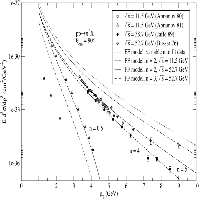
for any hadron $h$. Feynman fixed $n=2$ in his original paper. In this work, $n$ is a parameter freely adjusted to fit data. There is a subtlety involved in summing all the parton contributions over $a$ and $b$ in Eq. (216) that is related to the relative probabilitistic nature of the parton distributions. The best way to explain it is by the way of an analogy. Suppose there is a room $A$ occupied by 7 boys and 5 girls. The ratio of boys to girls in that room is 7:5, or ${7\over 12}:{5\over 12}$ in normalized format. Suppose there is another room $B$ of 14 boys and 10 girls. The ratio is also 7:5. If a superintendent wants to know the number of children in room $B$, it is not enough to know the ratio of boys to girls. He must also be given a integral multiplicative constant. In this case, 2 times 7:5 or 24 times ${7\over 12}:{5\over 12}$ gives the correct head counts which is 14:10. A similar situation arises in counting the number of partons in a hadron. The parton distributions are normalized to unity so that they give only the relative distributions of the partons. The parton distributions give only the ratios of the partons in a hadron but not their numbers. In order to sum over $a$ and $b$ partons in Eq. (216) correctly, one must be provided with an integral multiplicative constant for each of the hadrons $A$ and $B$. These multiplicative integral constants cannot be known a priorí but are determined a posteriorí by fitting data. In other words, Eq. (216) can be modified as

$$E\,{d^{3}\sigma\over dp^{3}} = {N_{A}\,N_{B}\over\pi}\,\sum_{\{a,b\}}\,\int^{1}_{x_{a}^{min}}dx_{a}\int^{1}_{x_{b}^{min}}dx_{b}$$ (239)

$$\quad\times f_{A/a}(x_{a},Q^{2})\,f_{B/b}(x_{b},Q^{2})\,D^{h}_{c}(z_{c},Q^{2})\,{1\over z_{c}}\,{d\hat{\sigma}\over d\hat{t}},$$

where $N_{A}$ and $N_{B}$ are the multiplicative constants corresponding to $f_{A/a}(x_{a},Q^{2})$ and $f_{B/b}(x_{b},Q^{2})$ respectively and $\sum_{\{a,b\}}$ is the sum over the parton types instead of a sum over the partons per se. If $A=B$, the overall multiplicative constant, $N_{A}\,N_{B}$, is an integer square. If $A\neq B$, the overall constant, $N_{A}\,N_{B}$, is still an integer. In the case of fitting the pQCD calculations to experimental data of the $pp\to\pi\,X$ reaction, a factor of 100 is missing if one simply sums over the parton types. It implies that the multiplicative constant for the parton distributions of proton is $N_{p}=10$. The cross sections for $K$ production is approximately half of that of $\pi$ production. It implies that the multiplicative constant for the $pp\to K\,X$ reaction is $N_{p}=7$. For the purpose parameterizing the shape of the kaon production cross section, the exact value of the scale is not required. Therefore $N_{p}$ in the $pp\to KX$ reactions is arbitrarily set to be the same as that of $pp\to\pi X$ reactions at $N_{p}=10$. This choice is adequate because fits to kaon experimental data are not being pursued due to a lack of experimental data.

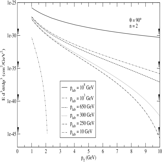
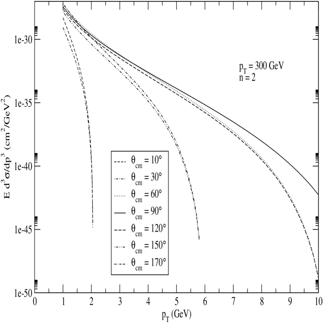
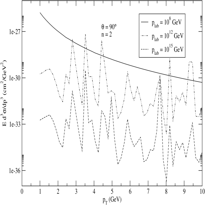
Figures 1 and 2 illustrate the features of $E\,d^{3}\sigma/dp^{3}$ plotted against $p_{T}$. Fig. 1 shows that the invariant cross section is visibly suppressed at high $p_{T}$. Fig. 2 shows that the suppression increases as $\theta_{cm}$ moves farther away from $90^{\circ}$ and that the suppression is symmetric around $\theta_{cm}=90^{\circ}$. Fig. 3 shows that the Monte Carlo code is plagued by numerical noise at excessively high $\sqrt{s}$. These illustrations summarize the global properties of the invariant production of cross sections of pions and kaons.

It is observed that the invariant production cross sections have the same basic shape regardless of the reactions, i.e. an exponentially decaying function of the form $\exp(-\alpha x^{\beta})$ at low $p_{T}$ and a suppression at high $p_{T}$ which drops off to zero before the edge of suppresion at $p_{T}\leq\sqrt{s}/2$. The cross section is at its maximum at $p_{T}=0$ and decreases monotonically in $p_{T}$. The Feynman-Field code used in this calculation assumes that $Q^{2}=4p_{T}^{2}$. In other words, by combining the previous two statements, the cross section is at its maximum at $Q^{2}=0$ and decreases monotonically in $Q^{2}$. This observation indicates that hadron fragmentation is more favorable at low $Q^{2}$ in that a parton preserves more kinetic energy to be made available for hadron fragmentation. It is also observed that the cross section is suppressed at high $p_{T}$ and that the edge of suppression of the cross section is $\sqrt{s}/2$ at low $p_{T}$ and gradually increases toward high $p_{T}$. The reason for this phenomenon is mostly due to the choice of $Q^{2}=4p_{T}$ such that $s\geq Q^{2}$ or equivalently $\sqrt{s}/2\geq p_{T}$. It turns out that the edge of suppression along $p_{T}$ is a function of $\sqrt{s}$. The comments made so far apply to any angle $\theta_{cm}$ when $\sqrt{s}$ is replaced by $\sin\theta\sqrt{s}$. These observations will be incorporated into the parameterization described in the next section.

3.5 Monte Carlo Integration

A sample ANSI-C Monte Carlo program that calculates $E\,d^{3}\sigma/dp^{3}$ written in using the vegas routine is given below. The standard Monte Carlo integration packages are taken from Numerical Recipes [3]. They include vegas2.c, rebin.c and ran2.c. The Numeical Recipes packages need the header files nrutil.h, nr.h and nrutil.c to run. The CTEQ6 package is downloadable from the web at $\underline{http://www.cteq.org}$. The original package is written in fortran but is translated to C using f2c. The translated CTEQ6 package is contained in the file Ctq6Pdf.c. The f2c libraries must be installed in the system for the translator to work. When the code is compiled in unix/linux, the following line must be typed at the command prompt to link the f2c libraries to the executable:

    $$ gcc -o pip pip.c -lf2c -lm

where pip.c is the filename of the program.

Below is a sample code that calculates the invariant production cross section of the $pp\to\pi^{+}X$ reaction.

*******************************************************************
#include <stdio.h>
#include <math.h>
#define NRANSI
#include "/recipes/c_d/nrutil.h"
#include "/recipes/c_d/nr.h"
#include "/recipes/c_d/nrutil.c"
#include "/recipes/c_d/vegas2.c"
#include "/recipes/c_d/rebin.c"
#include "/recipes/c_d/ran2.c"
#include "Ctq6Pdf.c"
#define pi 3.1415926535897932384626433
#define lambda2 0.16                            /* part of alpha_s */
#define nf 5.0                      /* number of flavors (topless) */
#define beta 0.4             /* part of the fragmentation function */
#define fac 3.893792923e-28      /* conversion from GeV^-2 to cm^2 */

long idum;

void vegas(double regn[], int ndim, double (*fxn)(double [], double),
Ψ   int init, unsigned long ncall, int itmx, int nprn,
Ψ   double *tgral, double *sd, double *chi2a);
double fxn(double *x, double wt);
doublereal ctq6pdf_(integer *iparton, doublereal *x, doublereal *q);
int setctq6_(integer *iset);
int readtbl_(integer *nu);
integer nextun_(void);
int polint_(doublereal *xa, doublereal *ya, integer *n,
Ψ    doublereal *x, doublereal *y, doublereal *dy);
doublereal partonx6_(integer *iprtn, doublereal *xx, doublereal *qq);

double x1,x2,s,t,u,Q2,as2;
float plab,d;
integer *ipartona,*ipartonb;
doublereal *q;

MAIN__(void)
{
  int t1,t2,t3,ndim=2,i,imax,init=0,ncall=5000,itmx=5,nprn=0;
  int n=2*ndim;
  integer *iset;
  double pT,dpT,pTmin=1.0,xT,Th;
  float pTmax,tmp;
  double *regn;
  double alo,as,theta;
  double *tgral,*sd,*chi2a;
  FILE *fp;

  regn=dvector(1,n);
  tgral=dvector(1,1);
  sd=dvector(1,1);
  chi2a=dvector(1,1);
  ipartona=lvector(1,1);
  ipartonb=lvector(1,1);
  q=dvector(1,1);

  *iset=1L;                                /* CTEQ6 for MSbar */
  fp=fopen("out.dat","w");

  printf("plab = ");
  scanf("%f",&plab);
  printf("theta = ");
  scanf("%f",&tmp);
  printf("d = ");
  scanf("%f",&d);
  printf("pTmax = ");
  scanf("%f",&pTmax);
  printf("length (10 or 100): ");
  scanf("%d",&imax);

  t1=time(0);

  setctq6_(iset);          /* initialization for CTEQ6 routines */
  dpT=(pTmax-pTmin)/imax;
  pT=pTmin;
  theta=tmp*pi/180.0;
  s=2.0*0.938272*plab;
  Th=tan(theta/2.0);
  regn[3]=1.0;                                        /* xa_max */
  regn[4]=1.0;         /* xb_max */

  t2=time(0);

  for(i=0;i<=imax;i++) {
    Q2=4.0*pT*pT;
    q[1]=sqrt(Q2);
    alo=12.0*pi/(33.0-2.0*nf)/log(Q2/lambda2);
    as=alo*(1.0-(306.0-38.0*nf)/4.0/pi/(33.0-2.0*nf)*alo
Ψ*log(log(Q2/lambda2)));
    as2=as*as;
    xT=2.0*pT/sqrt(s);
    x1=0.5*xT/Th;
    x2=0.5*xT*Th;
    t=-s*x2;
    u=-s*x1;
    regn[1]=x1/(1.0-x2); /* xa_min */
    regn[2]=x2/(1.0-x1); /* xb_min */
    vegas(regn, ndim, fxn, init, ncall, itmx, nprn,
Ψ  &tgral[1], &sd[1], &chi2a[1]);
    fprintf(fp,"%f\t%e\n",pT,fac*tgral[1]*100.0);
    pT+=dpT;
  }

  t3=time(0);

  fclose(fp);
  free_dvector(regn,1,n);
  free_dvector(tgral,1,1);
  free_dvector(sd,1,1);
  free_dvector(chi2a,1,1);
  free_lvector(ipartona,1,1);
  free_lvector(ipartonb,1,1);
  free_dvector(q,1,1);
  printf("\ntime used for overheads = %d seconds\n",t2-t1);
  printf("\ntime used for integrals = %d seconds\n\n\a",t3-t2);
}

double fxn(double *x, double wt) {
  double cs,z,Fbar,f,tmp;
  double sh,th,uh;        /* internal mandelstam vars */
  double sh2,th2,uh2;
  double M1,M2,M3,M4,M5;  /* inv amp */
  double Du,Dd,Ds;        /* fragmentation functions */

  z=x2/x[2]+x1/x[1];
  sh=x[1]*x[2]*s;
  th=x[1]*t/z;
  uh=x[2]*u/z;
  sh2=sh*sh;
  th2=th*th;
  uh2=uh*uh;
  M1=4.0/9.0*(sh2+uh2)/th2;
  M2=4.0/9.0*((sh2+uh2)/th2+(sh2+th2)/uh2)-8.0/27.0*sh2/uh/th;
  M3=4.0/9.0*((sh2+uh2)/th2+(th2+uh2)/sh2)-8.0/27.0*uh2/sh/th;
  M4=(uh2+th2)/uh/th/6.0-3.0/8.0*(uh2+th2)/sh2;
  M5=-4.0/9.0*(uh2+sh2)/uh/sh+(uh2+sh2)/th2;
  f=(d+1.0)*pow(1.0-z,d);
  Fbar=(1.0/z-1.0)*f;
  Ds=Dd=beta*beta*Fbar;
  Du=beta*f+Ds;

  if (x[2]<x[1]*x2/(x[1]-x1)) cs=0.0;
  else {
    cs=0.0;

    /* su->s */
    ipartona[1]=3L;
    ipartonb[1]=1L;
    cs+=ctq6pdf_(&ipartona[1],&x[1],&q[1])
Ψ*ctq6pdf_(&ipartonb[1],&x[2],&q[1])*M1*Ds;

    /* subar->s */
    ipartona[1]=3L;
    ipartonb[1]=-1L;
    cs+=ctq6pdf_(&ipartona[1],&x[1],&q[1])
Ψ*ctq6pdf_(&ipartonb[1],&x[2],&q[1])*M1*Ds;

    /* us->u */
    ipartona[1]=1L;
    ipartonb[1]=3L;
    cs+=ctq6pdf_(&ipartona[1],&x[1],&q[1])
Ψ*ctq6pdf_(&ipartonb[1],&x[2],&q[1])*M1*Du;

    /* usbar->u */
    ipartona[1]=1L;
    ipartonb[1]=-3L;
    cs+=ctq6pdf_(&ipartona[1],&x[1],&q[1])
Ψ*ctq6pdf_(&ipartonb[1],&x[2],&q[1])*M1*Du;

    /* ub->u */
    ipartona[1]=1L;
    ipartonb[1]=5L;
    cs+=ctq6pdf_(&ipartona[1],&x[1],&q[1])
Ψ*ctq6pdf_(&ipartonb[1],&x[2],&q[1])*M1*Du;

    /* ubar->u */
    ipartona[1]=1L;
    ipartonb[1]=-5L;
    cs+=ctq6pdf_(&ipartona[1],&x[1],&q[1])
Ψ*ctq6pdf_(&ipartonb[1],&x[2],&q[1])*M1*Du;

    /* uc->u */
    ipartona[1]=1L;
    ipartonb[1]=4L;
    cs+=ctq6pdf_(&ipartona[1],&x[1],&q[1])
Ψ*ctq6pdf_(&ipartonb[1],&x[2],&q[1])*M1*Du;

    /* ucbar->u */
    ipartona[1]=1L;
    ipartonb[1]=-4L;
    cs+=ctq6pdf_(&ipartona[1],&x[1],&q[1])
Ψ*ctq6pdf_(&ipartonb[1],&x[2],&q[1])*M1*Du;

    /* sd->s */
    ipartona[1]=3L;
    ipartonb[1]=2L;
    cs+=ctq6pdf_(&ipartona[1],&x[1],&q[1])
Ψ*ctq6pdf_(&ipartonb[1],&x[2],&q[1])*M1*Ds;

    /* sdbar->s */
    ipartona[1]=3L;
    ipartonb[1]=-2L;
    cs+=ctq6pdf_(&ipartona[1],&x[1],&q[1])
Ψ*ctq6pdf_(&ipartonb[1],&x[2],&q[1])*M1*Ds;

    /* sb->s */
    ipartona[1]=3L;
    ipartonb[1]=5L;
    cs+=ctq6pdf_(&ipartona[1],&x[1],&q[1])
Ψ*ctq6pdf_(&ipartonb[1],&x[2],&q[1])*M1*Ds;

    /* sbbar->s */
    ipartona[1]=3L;
    ipartonb[1]=-5L;
    cs+=ctq6pdf_(&ipartona[1],&x[1],&q[1])
Ψ*ctq6pdf_(&ipartonb[1],&x[2],&q[1])*M1*Ds;

    /* sc->s */
    ipartona[1]=3L;
    ipartonb[1]=4L;
    cs+=ctq6pdf_(&ipartona[1],&x[1],&q[1])
Ψ*ctq6pdf_(&ipartonb[1],&x[2],&q[1])*M1*Ds;

    /* scbar->s */
    ipartona[1]=3L;
    ipartonb[1]=-4L;
    cs+=ctq6pdf_(&ipartona[1],&x[1],&q[1])
Ψ*ctq6pdf_(&ipartonb[1],&x[2],&q[1])*M1*Ds;

    /* ds->d */
    ipartona[1]=2L;
    ipartonb[1]=3L;
    cs+=ctq6pdf_(&ipartona[1],&x[1],&q[1])
Ψ*ctq6pdf_(&ipartonb[1],&x[2],&q[1])*M1*Dd;

    /* dsbar->d */
    ipartona[1]=2L;
    ipartonb[1]=-3L;
    cs+=ctq6pdf_(&ipartona[1],&x[1],&q[1])
Ψ*ctq6pdf_(&ipartonb[1],&x[2],&q[1])*M1*Dd;

    /* db->d */
    ipartona[1]=2L;
    ipartonb[1]=5L;
    cs+=ctq6pdf_(&ipartona[1],&x[1],&q[1])
Ψ*ctq6pdf_(&ipartonb[1],&x[2],&q[1])*M1*Dd;

    /* dbbar->d */
    ipartona[1]=2L;
    ipartonb[1]=-5L;
    cs+=ctq6pdf_(&ipartona[1],&x[1],&q[1])
Ψ*ctq6pdf_(&ipartonb[1],&x[2],&q[1])*M1*Dd;

    /* dc->d */
    ipartona[1]=2L;
    ipartonb[1]=4L;
    cs+=ctq6pdf_(&ipartona[1],&x[1],&q[1])
Ψ*ctq6pdf_(&ipartonb[1],&x[2],&q[1])*M1*Dd;

    /* dcbar->d */
    ipartona[1]=2L;
    ipartonb[1]=-4L;
    cs+=ctq6pdf_(&ipartona[1],&x[1],&q[1])
Ψ*ctq6pdf_(&ipartonb[1],&x[2],&q[1])*M1*Dd;

    /* ud->u */
    ipartona[1]=1L;
    ipartonb[1]=2L;
    cs+=ctq6pdf_(&ipartona[1],&x[1],&q[1])
Ψ*ctq6pdf_(&ipartonb[1],&x[2],&q[1])*M1*Du;

    /* udbar->u */
    ipartona[1]=1L;
    ipartonb[1]=-2L;
    cs+=ctq6pdf_(&ipartona[1],&x[1],&q[1])
Ψ*ctq6pdf_(&ipartonb[1],&x[2],&q[1])*M1*Du;

    /* du->d */
    ipartona[1]=2L;
    ipartonb[1]=1L;
    cs+=ctq6pdf_(&ipartona[1],&x[1],&q[1])
Ψ*ctq6pdf_(&ipartonb[1],&x[2],&q[1])*M1*Dd;

    /* dubar->d */
    ipartona[1]=2L;
    ipartonb[1]=-1L;
    cs+=ctq6pdf_(&ipartona[1],&x[1],&q[1])
Ψ*ctq6pdf_(&ipartonb[1],&x[2],&q[1])*M1*Dd;

    /* uu->u */
    ipartona[1]=1L;
    ipartonb[1]=1L;
    cs+=ctq6pdf_(&ipartona[1],&x[1],&q[1])
Ψ*ctq6pdf_(&ipartonb[1],&x[2],&q[1])*M2*Du;

    /* dd->d */
    ipartona[1]=2L;
    ipartonb[1]=2L;
    cs+=ctq6pdf_(&ipartona[1],&x[1],&q[1])
Ψ*ctq6pdf_(&ipartonb[1],&x[2],&q[1])*M2*Dd;

    /* ss->s */
    ipartona[1]=3L;
    ipartonb[1]=3L;
    cs+=ctq6pdf_(&ipartona[1],&x[1],&q[1])
Ψ*ctq6pdf_(&ipartonb[1],&x[2],&q[1])*M2*Ds;

    /* uubar->u */
    ipartona[1]=1L;
    ipartonb[1]=-1L;
    cs+=ctq6pdf_(&ipartona[1],&x[1],&q[1])
Ψ*ctq6pdf_(&ipartonb[1],&x[2],&q[1])*M3*Du;

    /* ddbar->d */
    ipartona[1]=2L;
    ipartonb[1]=-2L;
    cs+=ctq6pdf_(&ipartona[1],&x[1],&q[1])
Ψ*ctq6pdf_(&ipartonb[1],&x[2],&q[1])*M3*Dd;

    /* ssbar->s */
    ipartona[1]=3L;
    ipartonb[1]=-3L;
    cs+=ctq6pdf_(&ipartona[1],&x[1],&q[1])
Ψ*ctq6pdf_(&ipartonb[1],&x[2],&q[1])*M3*Ds;

    /* gg->u,d,s */
    ipartona[1]=0L;
    ipartonb[1]=0L;
    cs+=ctq6pdf_(&ipartona[1],&x[1],&q[1])
Ψ*ctq6pdf_(&ipartonb[1],&x[2],&q[1])*M4*(Du+Dd+Ds);

    /* ug->u */
    ipartona[1]=1L;
    ipartonb[1]=0L;
    cs+=ctq6pdf_(&ipartona[1],&x[1],&q[1])
Ψ*ctq6pdf_(&ipartonb[1],&x[2],&q[1])*M5*Du;

    /* dg->d */
    ipartona[1]=2L;
    ipartonb[1]=0L;
    cs+=ctq6pdf_(&ipartona[1],&x[1],&q[1])
Ψ*ctq6pdf_(&ipartonb[1],&x[2],&q[1])*M5*Dd;

    /* sg->s */
    ipartona[1]=3L;
    ipartonb[1]=0L;
    cs+=ctq6pdf_(&ipartona[1],&x[1],&q[1])
Ψ*ctq6pdf_(&ipartonb[1],&x[2],&q[1])*M5*Ds;

    cs*=as2/sh2/z;
  }
  return cs;
}

#undef NRANSI

4 Conclusion

The Lund and Feynman-Field models are derived and implemented numerically in this work. New results based on these models will published as a separate paper.

Figure 1: A sample plot of the Feynman-Field model for $pp\to\pi^{+}X$ at different energies and $\theta_{cm}=90^{\circ}$. The plot shows that the invariant cross section is suppressed at high $p_{T}$.

Figure 2: A sample plot of the Feynman-Field model for $pp\to\pi^{+}X$ at different angles. The plot shows that the invariant cross section is symmetric around $\theta_{cm}=90^{\circ}$ and is suppressed at $\theta_{cm}\neq 90^{\circ}$.

Figure 3: A sample plot of the Feynman-Field model for $pp\to\pi^{+}X$ at excessively high energies and $\theta_{cm}=90^{\circ}$. The plot shows that the Monte Carlo code breaks down at ultra-high energies.

Figure 4: Comparisons of the Feynman-Field model fit for $pp\to\pi^{+}X$ for various $n$ at $\theta_{cm}=90^{\circ}$. The references of the data sets Abromov 80, Abramov 81, Jaffe 89 and Busser 76 are Nuclear Phys., B173 348 (1980), ZETFP 33 304 (1981), Phys. Rev., D40 2777 (1989) and Nuclear Phys., B106 1 (1976) respectively.

Figure 5: The yoyo motion of a quark-antiquark pair confined by a linear potential. The two quarks are assumed to be massless. The mass square of the meson is proportional to the area of each square. The meson shown here is at rest.

Figure 6: The breakup of a quark-antiquark pair along a surface of constant proper time $\tau$. The bold arrows represents the velocities of the produced mesons. The breakup points are labelled as vertices $V_{1}$ to $V_{n}$.

Figure 7: The geometry of the kinematics of two adjacent vertices $V_{1}$ and $V_{2}$. $V_{1}$ and $V_{2}$ are vertices or spacetime positions which also represent the energy carried by the string field. The quark moves along the positive light-cone and the antiquark moves along the negative light-cone. The antiquark of $V_{1}$ combines with the quark of $V_{2}$ to produce a meson of mass $m$. $W_{+1}$ is the energy of $V_{1}$ along $x_{+}$. $z_{+}W_{+1}$ is the fraction of energy used to create a quark from $V_{2}$. $W_{-2}$ is the energy of $V_{2}$ along $x_{-}$. $z_{-}W_{-2}$ is the fraction of energy used to create an antiquark from $V_{1}$. $A_{1}$, $A_{2}$, $A_{3}$ and $m^{2}$ are the areas of the rectangles. The figure is taken from reference [1].

Figure 8: The geometry of the kinematics of involving the total area of the spacetime diagram such that $A_{total}=\Gamma+A_{rest}$. The total energy square $s=W_{+}W_{-}$ is represented by the rectangle labelled $s$. $p_{\pm}$ is the energy of the parent quark (antiquark) along the $\pm$ light-cone coordinates. $z_{0n}p_{+}$ is the fraction of energy used to create a quark from $V_{n}$. $m^{2}/(z_{0n}p_{+})$ is the energy used to create an antiquark from $V_{n-1}$. The figure is taken from reference [1] with minor modifications.

Figure 9: Parton $a$ of hadron $A$ collides with parton $b$ of hadron $B$ producing partons $c$ and $d$. The transverse momenta, $p_{T}$, of $c$ and $d$ are equal and opposite.

Figure 10: The plot of $x_{a}$ versus $x_{b}$ with $x_{b}=x_{a}x_{2}/(x_{a}-x_{1})$. $x^{min}_{a}=x_{1}/(1-x_{2})$. The values of $x_{1}=0.5$ and $x_{2}=0.3$ are used.

References

- [1] B. Andersson, The Lund Model., (Cambridge Univ. Press, 1998).
- [2] R. D. Field, Applications of Perturbative QCD, (Addison-Wesley, 1989).
- [3] W. H. Press, S. A. Teukolsky, W. T. Vetterling and B. P. Flannery, Numerical Recipes in C, (Cambridge: Cambridge, 1997).
- [4] A. Tang, “Topics in Hadronic Physics,” Ph. D. dissertation, Physics Department, University of Wisconsin-Milwaukee (December 2002).
- [5] J. Polchinski, Introduction to String Theory, (Cambridge Univ. Press, 1998).
- [6] B. Hatfield, Quantum Field Theory of Point Particles and Strings, (Addison-Wesley, 1992).
- [7] B. Andersson, S. Mohanty and F. Söderberg, hep-ph/0106185, (16 June 2001).
- [8] V. V. Abramov, et al., Nuclear Phys., B173, 348 (1980).
- [9] G. P. Lepage, Cornell University Publication, CLNS-80/447 (1980).
- [10] J. Pumplin, D. R. Stump, J. Huston, H. L. Lai, P. Nadolsky, and W. K. Tung, hep-ph/0201195 (22 January 2002).
- [11] S. R. Blattnig, S. R. Swaminathan, A. T. Kruger, M. Ngom and J. W. Norbury, NASA Technical Paper, NASA/TP-2000-210640, (December 2000).
- [12] R. D. Field and R. P. Feynman, Nuclear Phys., B136, 1-76 (1978).
- [13] B. L. Combridge, J. Kripfganz and J. Ranft, Phys. Lett., 70B, 2, 234-238 (26 September 1977).