Quark-Hadron Duality

Abstract

Quark-hadron duality and its potential applications are discussed. We focus on theoretical efforts to model duality.

1 What is Duality?

In general, duality implies a situation in which two different languages give an accurate description of Nature. While one may be more convenient than the other in certain situations, both are correct. If we are interested in hadronic reactions, the two relevant pictures are the quark-gluon picture and the hadronic picture. In principle, we can describe any hadronic reaction in terms of quarks and gluons, by solving Quantum Chromodynamics (QCD). While this statement is obvious, it rarely has practical value, since in most cases we can neither perform nor interpret a full QCD calculation. In general, we also cannot perform a complete hadronic calculation. We will refer to the statement that, if one could perform and interpret the calculations, it would not matter at all which set of states - hadronic states or quark-gluon states - was used, as ”degrees of freedom” duality.

However, there are cases where another, more practical form of duality applies: for some reactions, in a certain kinematic regime, properly averaged hadronic observables can be described by perturbative QCD (pQCD). This statement is much more practical than the ”degrees of freedom” duality introduced above. In contrast to full QCD, pQCD calculations can be performed, and in this way, duality can be exploited and applied to many different reactions.

Duality in the latter form was first found by Bloom and Gilman in 1970 in inclusive, inelastic electron scattering [1]. Duality in this reaction is therefore commonly referred to as Bloom-Gilman duality. Recently, it was impressively confirmed to high accuracy in measurements carried out at Jefferson Lab [2].

Duality also appears in the semileptonic decay of heavy quarks [3, 4], in the reaction $e^{+}e^{-}\rightarrow hadrons$ [5], in dilepton production in heavy ion reactions [6], and in hadronic decays of the $\tau$ lepton [7].

Why should one be interested in duality? It is not only a rather interesting and surprising phenomenon, but also has many promising applications, e.g. for experiments probing the valence structure of the nucleon [8]. In inclusive electron scattering, duality establishes a connection between the resonance region and the deep inelastic region. Measurements in the resonance region have higher count rates than measurements in the deep inelastic region, and duality might be able to open up previously inaccessible regions. New duality experiments have been completed or are currently carried out at Jefferson Lab [9, 8], and there will be a large duality program at the 12 GeV upgrade of CEBAF [10]. Examples of duality and possible applications of duality will be discussed in the next section.

In order to use duality confidently to extract information from experimental data, a good understanding of duality is necessary. We need to know where it holds and how accurate it is. Our current understanding of duality is still limited. The theoretical efforts focus on modelling duality, and are discussed in Section 3.

2 Applications and Examples

Our main focus is duality in electron scattering. We will briefly review duality in other reactions, before turning to the main subject of the talk.

2.1 Duality in various reactions

For semileptonic decays of heavy quarks, duality implies that the decay rate for hadrons is determined by the decay rate of the underlying quark decay. For perfect duality, the quark decay rate $b\rightarrow cl\bar{\nu}_{l}$ is equal to the sum over all hadronic decays, $\bar{B}\rightarrow X_{c}l\bar{\nu_{l}}$, where $X_{c}$ stands for the ground state $D$ meson and its excited states. For infinitely heavy masses of the $b$ and $c$ quarks, duality was shown to hold exactly. In the realistic case of heavy, but not infinitely heavy quarks $M_{q}$, the various observables pick up correction terms of order $\frac{1}{M_{q}}$ and $\frac{1}{M_{q}^{2}}$. The precise form of the correction, in particular the question if $\frac{1}{M_{q}}$ corrections exist at all, was the subject of much debate in the literature, see e.g. [11]. It seems that this matter was resolved recently in [4], where it was shown that the form of the correction depends on the observable.

The reaction $e^{+}e^{-}\rightarrow hadrons$ is a famous example of duality [12, 5]. Using the optical theorem, the cross section for the process can be described as the imaginary part of the forward elastic scattering amplitude, where the latter either contains a sum over all possible hadrons, i.e. the vector mesons, or a sum over quark loops, including interactions with hard and soft gluons. For high enough center of mass energies, the ratio of the hadronic cross section to the $e^{+}e^{-}\rightarrow\mu^{+}\mu^{-}$ cross section is equal to $N_{c}\sum_{q}e_{q}^{2}$, where $N_{c}$ is the number of colors and $e_{q}$ is the electric charge of a quark of flavor $q$. This clearly shows that at these energies, one may use either the quark degrees of freedom or hadronic degrees of freedom. More surprising, even at low center of mass energies where the resonance bumps can be seen clearly, the ”quark result” $N_{c}\sum_{q}e_{q}^{2}$, describes the average of the ratio.

The production of dilepton pairs is the inverse reaction to $e^{+}e^{-}\rightarrow hadrons$. One prominent feature of the dilepton production rate is the broadening of the resonance peaks in the spectrum, which gave rise to the explanation that the vector meson masses drop in the medium ”dropping $\rho$-mass”. This phenomenon has also been interpreted as a quark-hadron duality induced effect [13, 6]. Just as the resonance peaks vanish for masses larger than 1.5 GeV and below the $J/\Psi$ threshold (i. e. when the only active flavors are $u$, $d$, and $s$), the resonance peaks vanish in the dilepton production. Here, this vanishing occurs at lower masses already, which was interpreted [6] as an in-medium reduction of the quark-hadron duality scale of $1.5$ GeV for active $u,d,$ and $s$ flavors. Calculations working with hadronic degrees of freedom and quark-gluon degrees of freedom produce the same effect.

2.2 Duality in inclusive electron scattering

The cross section for inclusive electron scattering is given by $\frac{d\sigma}{d\Omega dE_{f}}=\sigma_{Mott}(W_{2}+2W_{1}\tan^{2}{\frac{\vartheta_{e}}{2}})\,,$ where $\sigma_{Mott}\propto Q^{-4}$. Therefore, the cross section for high $Q^{2}$ is dropping off rapidly. Traditionally, the region where $W$, the invariant mass of the final state, is smaller than 2 GeV, is called the resonance region, and $W>2$ GeV is referred to as the deep inelastic region. This distinction is rather artificial, and one key point of quark-hadron duality is that these two regions are actually connected. It is clear that duality in inclusive electron scattering must hold in the scaling region, for $Q^{2}\rightarrow\infty$, as perturbative QCD is valid there, and therefore will describe the hadronic reaction. In deep inelastic scattering, the kinematics are such that the struck quark receives so much energy over such a small space-time region that it behaves like a free particle during the essential part of its interaction. This leads to the compellingly simple picture that the electromagnetic cross section in this kinematic region is determined by free electron-quark scattering, i.e. duality is exact for this process in the scaling region. The really interesting question is if duality will be valid approximately at lower $Q^{2}$, in a region where the cross section is dominated by resonances, which are strongly interacting hadrons, after all. The experimental data, see Fig. 1, show that duality holds even at very low $Q^{2}\approx 0.5$ GeV² [2].

Figure 1: Experimental data for $F_{2}(\xi,Q^{2})=\nu W_{2}(\xi,Q^{2})$ from Jefferson Lab [2]. The data is plotted versus Nachtmann’s variable $\xi$.

One can see clearly that the resonance data follows the scaling curve, as given by the NMC parameterization evolved to $Q^{2}=5$ GeV ². In principle, one should compare the resonance results to the pQCD results evolved to the same $Q^{2}$ at which the resonance data were taken. As the resonance $Q^{2}$ values are too low for this, choosing 5 GeV² is a very reasonable approach. Finite energy sum rules formed for the scaling (pQCD) curve and the resonance regime further quantify the validity of duality, for details see [2]. Also, moments of the data have been considered [14]. The most striking feature of the moments is that they flatten out at rather low $Q^{2}\approx 2$ GeV ².

Figure 2: Left panel: Extracted values for the magnetic form factor of the proton, from [15]. Right panel: Data from SLAC for the polarization asymmetry of the neutron, $A_{1}^{n}$, and projected data for the Jefferson Lab experiment E01-012 [16].

If duality holds very locally, i.e. for just one resonance, instead of the whole resonance region, then one may use it to extract information on the resonance region from the deep inelastic region, and vice versa. A benchmark for applying duality in this, very local, way is the extraction of the magnetic form factor of the proton from the scaling curve [17, 15]. The result is shown in Fig. 2. The qualitative agreement is very good, and quantitatively, one sees that the duality extraction undershoots the form factor parameterization somewhat. This result may give us a good idea where we are in our understanding of duality, and in our ability to extract information from the data. One important caveat in this case is that here, $G_{M}^{p}$ was extracted from the $F_{2}$ data, and a constant ratio of 2.79 was assumed for the ratio of $G_{M}$ to $G_{E}$. As we know from recent Hall A data from Jefferson Lab [18], this is not a decent assumption, and may introduce a sizable error. The good news is that new data for $F_{1}$ have recently been taken at Jefferson Lab, and an extraction of $G_{M}$ can be performed without any assumptions on the ratio $G_{M}/G_{E}$, as in elastic scattering, the electric form factor does not enter into the purely transverse $F_{1}$.

pt 0.24 3 h:L v:C 4 (549 134)(569 134) (1436 134)(1416 134) (527 134)h:R v:C 0 (549 278)(569 278) (1436 278)(1416 278) (527 278) 0.2 (549 422)(569 422) (1436 422)(1416 422) (527 422) 0.4 (549 567)(569 567) (1436 567)(1416 567) (527 567) 0.6 (549 711)(569 711) (1436 711)(1416 711) (527 711) 0.8 (549 855)(569 855) (1436 855)(1416 855) (527 855) 1 (549 134)(549 154) (549 855)(549 835) (549 89)h:C v:C 0 (771 134)(771 154) (771 855)(771 835) (771 89) 5 (993 134)(993 154) (993 855)(993 835) (993 89) 10 (1214 134)(1214 154) (1214 855)(1214 835) (1214 89) 15 (1436 134)(1436 154) (1436 855)(1436 835) (1436 89) 20 (549 134)(1436 134)(1436 855)(549 855)(549 134) (360 494)x_Bj (992 -1)Q² (GeV²) (593 747)h:L v:C Resonance Region (771 278)Deep Inelastic Region 3 (549 134)(549 134)(593 309)(638 416)(682 488)(726 539) (771 578)(815 608)(859 633)(904 653)(948 669) (993 684)(1037 696)(1081 706)(1126 716)(1170 724) (1214 731)(1259 737)(1303 743)(1347 749)(1392 753) (1436 758)(1436 758)

Figure 3: The kinematic plane. The line indicates that W = 2 GeV. The region below it corresponds to W $>$ 2 GeV (deep inelastic region), the region above it corresponds to W $<$ 2 GeV (resonance region).

Now, while extracting $G_{M}$ from deep inelastic data is a good check of our methods, this is not necessarily the ”direction” we want to take. From a practical point of view, it is very interesting to learn about the deep inelastic region from the resonance data. The valence quark region, i.e. the region of $x_{Bj}$ close to 1, is of particular interest. However, data there are scarce, as the count rate in this kinematic region is very low. This can be seen immediately by inspecting Fig. 3, and recalling that $\sigma_{Mott}\propto Q^{-4}$. If one wants to measure in the deep inelastic region at large $x_{Bj}$, one necessarily has a very large $Q^{2}$. However, if one is interested in a measurement at the very same value of $x_{Bj}$ in the resonance region, the $Q^{2}$ values may be very small, and the count rate may therefore be much larger.

One interesting, but currently not very well known quantity is the polarization asymmetry of the neutron, $A_{1}^{n}$. For $x_{Bj}\rightarrow 1$, it contains information about the valence quark spin distribution functions. There exist various, widely differing predictions for this quantity, for a review, see [19]. If one believes that duality holds very locally, one may predict $A_{1}^{n}$ from form factor data [20]. As can be seen from Fig. 2, the currently existing data from SLAC (open symbols) are plagued by very large error bars, and do not reach the region of high $x_{Bj}$ relevant for the valence quarks. The filled symbols represent $projections$ for data that are currently taken at Jefferson Lab, exploiting duality [8]. This means that data would be taken in the resonance region, and then properly averaged to obtain information on the deep inelastic region. As can be seen, the data taken in this way would have a much higher precision than the presently existing SLAC data, and would be deep in the valence quark regime of high $x_{Bj}$. However, before we can apply such a ”duality procedure” to data from the resonance region, we must understand where exactly duality holds, how exact it is, and which averaging procedure needs to be applied. The latter is especially important for polarized measurements, as one will need to take care to average only over resonances with the correct quantum numbers. Currently, we do not yet have such a firm and quantitative understanding of duality. There are several groups working on improving our theoretical understanding of duality, which is the topic of the next section.

3 Search for the Origins of Duality

The main questions that need to be addressed from the theoretical side are: Why do we observe duality? How can we see precocious scaling in a region where the interactions are strong? And, very relevant to applications of duality: For which observables in which kinematic regimes can we apply quark-hadron duality, and how precise are our results going to be? Theoretical efforts can be divided into two categories: refinement of the data analysis, e.g. use of various scaling variables, Cornwall-Norton vs Nachtmann moments, target mass corrections, averaging [21, 14, 22], and modelling [23, 24, 25, 26]. I will focus on the latter for the rest of my talk.

When modelling duality, the first goal is to gain a qualitative understanding of the phenomenon. Obviously, the situation as observed in nature is very complicated, necessitating various simplifications. Nevertheless, the goal is to incorporate the essential physical features into a model. The general approach is to choose a solvable model for hadrons, calculate the relevant observables, and compare these results to the - hypothetical - free quark results. At this point, all models assume that after the excitation from the ground state to an excited level $N$, the quark will remain in its excited state,i.e. the produced resonance will not decay. The results obtained for the transition of the quarks to a bound, excited state are summed over and compared to the case where in the final state, the binding potential is switched off, and the quark is ”free”. The latter case corresponds to the pQCD situation. A schematic view of the modelling is given in Fig. 4.

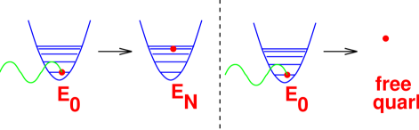
Figure 4: Schematic view of the model calculations. The left panel shows the bound-bound transition, the right panel shows the bound-free transition.

All models for duality must fulfill the following criteria:

1. The model must reproduce scaling. In addition, the scaling curve for the transition from the quark’s ground state to the excited state must lead to the same scaling curve as the transition from the ground state to a free quark state.

2. The calculated moments must flatten out for large $Q^{2}$, as observed in the data.

3. The resonance region results should oscillate around the scaling curve.

Let me now turn to one particular model, which was introduced in [23, 24]. The approach in this work was to construct a model with just a few underlying basic assumptions, which could be extended to the more realistic case. In [23, 24], we assumed that it is sufficient to incorporate relativity and confinement in a valence quark model. We also treated the quarks as scalars - while spin is crucial in nature, we assumed that for duality to be observed, it would not be necessary. In principle, we are interested in nucleon targets, i.e. in a three-body system. As this poses some technical difficulties, we assumed that only one quark would carry charge and therefore interact with the photon, the other two quarks form a spectator system. One may think of them either as an anti-quark or as a diquark. In order to further simplify the task, we also assumed that the spectator system has infinite mass. This means that instead of solving the Bethe-Salpeter equation for the two-body problem, we have to solve only a one-body equation. As we are dealing with scalar quarks, the Klein-Gordon equation needs to be solved. We model the confinement using a scalar, linear potential, $V\propto r$. As the potential enters the Klein-Gordon equation as $V^{2}$, the resulting equation resembles the Schrödinger equation for the non-relativistic harmonic oscillator. This has the advantage that the wave functions obtained in the solution are exactly the wave functions obtained for the non-relativistic harmonic oscillator, whereas the energy spectrum is given by $E_{N}\propto\sqrt{N}$, which leads to a much higher density of excited states than in the non-relativistic case, where $E_{N}^{non-rel}\propto N$. A comparison between the relativistic and the non-relativistic solutions is easily feasible in this case. A nice feature of this model is that the solutions can be obtained analytically. The two parameters needed for this model are the constituent quark mass, $m=0.33$ GeV and the string tension, which takes a value of $0.16$ GeV². None of the results depend crucially on these precise values, and we have checked that variation of these values gives reasonable results, e.g. we obtain the free case in the limit of the sting tension going to zero. While all particles, including beam and exchange particles, were treated as scalars in [23], only the quarks were treated as scalars in [24]. In the latter case, with spin $1/2$ electrons and spin $1$ photons, one deals with a conserved current.

The first requirement of duality that must be fulfilled by a model is scaling of the bound-bound transition, i.e. scaling for the case where only resonances are in the final state. Before investigating the scaling behavior, i.e. the behavior for large $Q^{2}$, we need to establish which quantity ought to scale, and which scaling variable to use. Bjorken’s variable $x_{Bj}=\frac{Q^{2}}{2M\nu}$ and scaling function $F_{2}=\nu W_{2}$ are designed for the region of $Q^{2}>>M^{2}$. Duality was observed to hold at much lower values of $Q^{2}$, where the target mass $M$ is about as large as $Q^{2}$, and the constituent quark mass, which is the relevant quantity at the considered low $Q^{2}$, is not negligible compared to $Q^{2}$. This situation demands a different scaling variable and scaling function. Bloom and Gilman used the ad hoc variable $x^{\prime}=\frac{Q^{2}}{W^{2}+Q^{2}}$, and later on [27], a variable that treats target mass and constituent quark mass on the same footing was derived. It reads $x_{cq}=\frac{1}{2M}(\sqrt{\nu^{2}+Q^{2}}-\nu)(1+\sqrt{1+\frac{4m^{2}}{Q^{2}}})$, and was derived for the case of free quarks with a momentum distribution. When deriving a scaling variable, it turns out that it is intimately connected to a scaling function, which for our case (scalar quarks), reads ${\cal{S}}_{2,cq}=|\vec{q}\,|W_{2}$. Note that all scaling variables and scaling functions must reduce to Bjorken’s variable $x_{Bj}$ and $F_{2}$ in the limit of high $Q^{2}$.

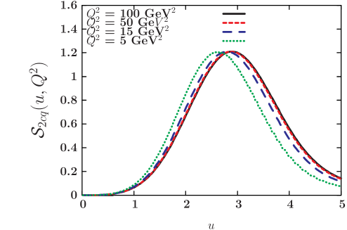
Figure 5: Scaling of the bound-bound transition for $Q^{2}\rightarrow\infty$.

The results for the scaling in the bound-bound case are shown in Fig. 5. It is clear from the figure that scaling is present: once $Q^{2}$ is high enough, the curves for different $Q^{2}$ practically coincide. Analytically, it was shown [24] that ${\cal{S}}_{2,cq}=\frac{m^{2}u_{Bj}^{2}}{\pi^{\frac{1}{2}}\beta E_{0}}\exp{\left(-\frac{(E_{0}-mu_{Bj})^{2}}{\beta^{2}}\right)}$, and that this is the same result which one obtains for the bound-free transition. It is interesting to note that the scaling function obtained in the all scalar case - where again, the bound-bound and bound-free transitions lead to the same scaling function - has a slightly different analytic form: ${\cal{S}}_{cq}=\frac{1}{4\pi^{\frac{1}{2}}\beta E_{0}}\exp{\left(-\frac{(E_{0}-mu_{Bj})^{2}}{\beta^{2}}\right)}\,.$ In the former case, one obtains that the scaling function goes to zero for the scaling variable approaching zero, as expected for valence quarks. However, we do not observe the behavior $\propto\sqrt{u}$, as predicted by Regge theory [28]. With our simple model, this was not to be expected, though, and it is interesting to observe how introducing the proper spin for the beam and exchange particles leads to a more realistic description. he moments flatten out at large $Q^{2}$, as required, and duality at low $Q^{2}$ is shown in Fig. 6 for the all scalar case (right panel) and the electromagnetic case (left panel).

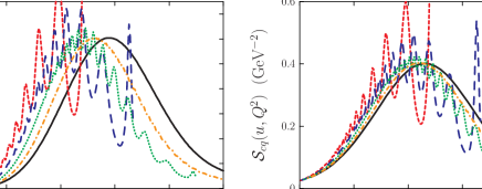
Figure 6: Duality at low $Q^{2}$ for the electromagnetic current (left panel), and the all scalar case (right panel). The solid lines show the result for large $Q^{2}$, the short dashed lines show $Q^{2}=0.5$ GeV², the long-dashed lines show $Q^{2}=1$ GeV², the dotted lines show $Q^{2}=2$ GeV², and the dash-dotted lines show $Q^{2}=5$ GeV².

A similar model is discussed in [25]. These authors consider a scalar probe and scalar quarks, and start from the semi-relativistic Hamiltonian ${\cal{H}}=\sqrt{\vec{p}\,^{2}}+\sqrt{\sigma}r$, where the quarks are massless. The solutions obtained in this approach are purely numerical. When considering scaling with respect to the many-body variable $\tilde{y}=\nu-|\vec{q}|$, scaling and local duality are observed. The authors also address the interesting question of contributions to sum rules from the time-like region, which may appear due to the binding of the quarks. The results in [25] differ in one important aspect from the results discussed previously [23, 24]: the bound-bound and bound-free transitions do not lead to the same scaling curves, they differ by about 30 %. This difference apparently stems from the different wave equations used for the two models.

4 Summary and Outlook

We have shown that duality appears in many reactions, is experimentally very well established, and has interesting and useful applications. Duality can be modelled, and with just a few basic assumptions, one can qualitatively reproduce all the features of duality. In the future, we will see more data exploring duality in various reactions - unpolarized and polarized reactions, and meson production. Theory will progress to more realistic models, including the spin of quarks and explicitly modelling the decay.

References

- [1] E. D. Bloom and F. J. Gilman, Phys. Rev. Lett. 25, 1140 (1970); E. D. Bloom and F. J. Gilman, Phys. Rev. D 4, 2901 (1971).
- [2] I. Niculescu et al., Phys. Rev. Lett. 85, 1182 (2000); 85, 1186 (2000); R. Ent, C.E. Keppel and I. Niculescu, Phys. Rev. D 62, 073008 (2000).
- [3] N. Isgur and M. B. Wise, Phys. Rev. D 43, 819 (1991).
- [4] R. Lebed and N. Uraltsev, Phys. Rev. D 62, 094011 (2000).
- [5] E. C. Poggio, H. R. Quinn, and S. Weinberg, Phys. Rev. D 13, 1958 (1976).
- [6] R. Rapp, hep-ph/0201101.
- [7] M. A. Shifman, arXiv:hep-ph/0009131.
- [8] Jefferson Lab experiment E01-012, spokespersons J.-P. Chen, S. Choi, and N. Liyanage; Jefferson Lab Experiment E93-009, spokespersons G. Dodge, S. Kuhn and M. Taiuti.
- [9] Contributions of E. Christy, C. Keppel, and I. Niculescu to these proceedings.
- [10] The Science driving the 12 GeV upgrade, edited by L. Cardman, R. Ent, N. Isgur, J.-M. Laget, C. Leemann, C. Meyer, and Z.-E. Meziani, Jefferson Lab, February 2001.
- [11] N. Isgur, Phys. Lett. B 448, 111 (1999).
- [12] see e.g. F. Halzen and A. D. Martin, ”Quarks & Leptons: An Introductory Course in Modern Particle Physics”, John Wiley & Sons, 1984.
- [13] see e.g. R. Rapp and J. Wambach, Adv. Nucl. Phys. 25, 1 (2000).
- [14] C. S. Armstrong, R. Ent, C. E. Keppel, S. Liuti, G. Niculescu and I. Niculescu, Phys. Rev. D 63, 094008 (2001).
- [15] R. Ent, C. E. Keppel and I. Niculescu, Phys. Rev. D 64, 038302 (2001).
- [16] N. Liyanage, private communication.
- [17] A. DeRujula, H. Georgi, and H. D. Politzer, Ann. Phys. (N.Y.) 103 315 (1977).
- [18] see e.g. Ed Brash, these proceedings.
- [19] N. Isgur, Phys. Rev. D 59, 034013 (1999).
- [20] W. Melnitchouk, Phys. Rev. Lett. 86, 35 (2001).
- [21] I. Niculescu, C. Keppel, S. Liuti and G. Niculescu, Phys. Rev. D 60, 094001 (1999); S. Liuti, R. Ent, C. E. Keppel and I. Niculescu, arXiv:hep-ph/0111063.
- [22] S. Simula, Phys. Lett. B 481, 14 (2000); Phys. Rev. D 64, 038301 (2001).
- [23] N. Isgur, S. Jeschonnek, W. Melnitchouk, and J. W. Van Orden, Phys. Rev. D 64, 054005 (2001).
- [24] S. Jeschonnek and J. W. Van Orden, Phys. Rev. D 65, 094038 (2002).
- [25] M. W. Paris and V. R. Pandharipande, Phys. Lett. B 514 361 (2001); M. W. Paris and V. R. Pandharipande, Phys. Rev. C 65, 035203 (2002).
- [26] F. Close and Q. Zhao, hep-ph/0202181.
- [27] R. Barbieri, J. Ellis, M. K. Gaillard, and G. G. Ross, Phys. Lett. 64B 171 (1976); R. Barbieri, J. Ellis, M. K. Gaillard, and G. G. Ross, Nucl. Phys. B117 50 (1976).
- [28] R. G. Roberts, ”The Structure of the Proton”, Cambridge University Press, 1990.