Vertex counting:
Statistical Distribution of Vertices
in Large Sets of Tree Diagrams
Petros Draggiotis and Ronald Kleiss
University of Nijmegen, the Netherlands
Abstract

We study the problem of determining the distribution of vertices of a particular given type in the set of all Feynman tree graphs in quantum field theories. We show that in almost all cases a Gaussian distribution arises asymptotically, and we compute the mean and variance of this distribution for several theories. We show the distribution’s ‘fine structure’, arising from topological sum rules, can be obtained.

1 Introduction

Recently, computational prowess in particle phenomenology has progressed to the evaluation of multi-particle scattering amplitudes, at least at the tree level, with ten or more external legs. The concomitant enormous number of Feynman graphs (e.g. 10.5 million for gluonic $2\to 8$ scattering) suggests the study of the Feynman graphs themselves as an ensemble of combinatorial objects. The number of graphs for various processes in self-interacting theories has been studied in a number of publications [1, 2], and also results for theories involving different particles have been found [3]. It is therefore natural to examine various statistical aspects of these ensembles more closely. In the present paper we deal with the problem of determining the frequecny of occurrence of particular vertices. For instance, one may wish to find the frequency of occurrence of four-gluon vertices in the ensemble of Feynman graphs for gluonic QCD: it is this kind of question that we address in this paper. The layout of the paper is as follows. First, we show that the frequency distribution of any kind of vertex tends to a Gaussian distribution as the number of external lines becomes asymptotically large. We then proceed to evaluate the parameters of these distributions for several theories, notably gluonic QCD and theories with all possible vertices present. These results hold for the ‘coarse-grained’ point of view in which the number of vertices is interpreted as a continuous, rather than a discrete, fraction of the number of legs. Subsequently, we discuss how the ‘fine structure’ of the distribution can be determined: this fine structure arises from the topological conservation laws that govern the number of vertices in any tree amplitude with a given number of legs. Finally, we turn to the more realistic case of QCD, in which both quark and gluon fields occur.

2 Gaussian limits for vertex occurrence

Consider a self-interacting theory of a single field $\varphi$. Since we will only be counting diagrams and vertices, the particular types of interactions are only important in terms of the number of legs involved in each vertex. We shall start with a quick review of the counting of diagrams. Let the theory have vertices of type $\varphi^{q+1}$ for some set of numbers $q\geq 2$ (that is, we allow any combination of 3,4,5,$\ldots$ vertices). We define the ‘potential’

$$W(\varphi)=\sum\limits_{q\geq 2}{\epsilon_{q}\over q!}\varphi^{q}$$ (1)

where $\epsilon_{q}=1$ if the vertex occurs in the action (or effective action), otherwise it is zero. If we denote the tree-level $1\to n$ amplitude by $a(n)$, we can define the amplitude-generating function by

$$\phi(x)=\sum\limits_{n\geq 1}{x^{n}\over n!}a(n)$$ (2)

Then, simple diagrammatic arguments [1] show that the Schwinger-Dyson equation for the number of diagrams is

$$\phi(x)=x+W(\phi(x))$$ (3)

Iteration of this relation, where $\phi(x)$ is a power series in $x$, then gives the number of graphs for any desired value of $n$; alternatively, the analytical structure of $\phi(x)$ as a function of $x$ informs us about the asymptotic behaviour of $a(n)$ with $n$. In particular, it is clear that in the general case $\phi(x)$ will be singular in $x$, and moreover that this singularity will be a branch cut rather than a pole. The condition for the singularity is, of course

$$\left|{d\phi(x)\over dx}\right|=\infty\;\;\Rightarrow\;\;{dx\over d\phi}=0\;\;\Rightarrow\;\;W^{\prime}(\phi)=1$$ (4)

Since $q\geq 2$ there are in general several solutions $\phi_{0}$ to this condition, and the radius of convergence of $\phi(x)$ as a power series is given by that solution $\phi_{0}$ which leads to the smallest absolute value of $x=\phi_{0}-W(\phi_{0})$. Taking this value of $\phi_{0}$, we see that, asymptotically, the number of graphs goes as

$$a(n)\sim{n!\over(\phi_{0}-W(\phi_{0}))^{n}}\;\;,$$ (5)

multiplied by subleading terms: in fact, the more precise form has been derived in [1] to read

$$a(n)\sim{n!\over n^{3/2}}{1\over(\phi_{0}-W(\phi_{0}))^{n}}\sqrt{{\phi_{0}-W(\phi_{0})\over 2\pi W^{\prime\prime}(\phi_{0})}}$$ (6)

but for the moment the leading form (5) is sufficient.

We now turn to the counting of vertices. Let us focus on the vertex of type $\varphi^{q+1}$ for some $q$ with $\epsilon_{q}=1$. We can count the occurrence of this vertex by giving it a weight $z$ in the Schwinger-Dyson equation (3), which then becomes

$$\phi(x,z)=x+W(\phi(x,z))+(z-1){\phi(x,z)^{q}\over q!}$$ (7)

The amplitude-generating function now depends on $z$ as well as on $x$. By iteration of this implicit equation we can find

$$\phi(x,z)=\sum\limits_{n\geq 1}{x^{n}\over n!}a(n;z)$$ (8)

to desired order in $x$. In the coefficient

$$a(n;z)=\sum\limits_{m\geq 0}b(n;m)z^{m}$$ (9)

which is a finite polynomial in $z$, the number $b(n;m)$ is then the number of $1\to n$ graphs with precisely $m$ vertices of type $\varphi^{q+1}$; and $a(n;1)$ is the total number of graphs. It is more instructive to consider not the number of graphs themselves but rather the probability to pick a diagram with $m$ $(q+1)$-vertices at random out of all tree graphs in the $1\to n$ amplitude. If we denote this probability by $\pi(n;m)$, we have simply

$$P_{n}(z)\equiv\sum\limits_{m\geq 0}\pi(n;m)z^{m}={a(n;z)\over a(n;1)}\;\;.$$ (10)

Putting in the leading asymptotic behaviour for $a(n)$ of Eq.(5) we therefore find that

$$\sum\limits_{m\geq 0}\pi(n;m)z^{m}\sim\left({F(\phi_{0}(1);1)\over F(\phi_{0}(z);z)}\right)^{n}\;\;\;,\;\;\;F(\varphi;z)\equiv\varphi-W(\varphi)-(z-1){\varphi^{q}\over q!}$$ (11)

and $\phi_{0}(z)$ is of course the value of $\phi(x;z)$ at the singularity nearest to the origin in the complex $x$ plane:

$$W^{\prime}(\phi_{0}(z))-(z-1){\phi_{0}(z)^{q-1}\over(q-1)!}=1\;\;.$$ (12)

The distribution of the $m$ values is determined once we know its moment-generating (or characteristic) function. It is simply related to the result we have obtained:

$$\left\langle e^{m\xi}\right\rangle \equiv \sum\limits_{k\geq 0}{\xi^{k}\over k!}\left\langle m^{k}\right\rangle=\sum\limits_{m,k\geq 0}\;\pi(n;m)\;{m^{k}\xi^{k}\over k!}$$ (13)

$$= \sum\limits_{m\geq 0}\;\pi(n;m)\;(e^{\xi})^{m}=\left({F(\phi_{0}(1);1)\over F(\phi_{0}(e^{\xi});e^{\xi})}\right)^{n}$$

But, by elementary arguments from probability theory, this implies that $m$ is distributed as the sum of $n$ independent, identically distributed random variables. The central limit theorem therefore asserts (except in special cases to which we shall come later) that for large $n$, the values of $m$ are normally distributed:

$$\pi(n;m)\sim{1\over\sqrt{2\pi n\sigma^{2}}}\exp\left(-{n\over 2\sigma(q)^{2}}\left({m\over n}-\mu(q)\right)^{2}\right)$$ (14)

with the parameters $\mu(q)$ and $\sigma(q)^{2}$ still to be determined (note that since $m$ is always integer, it is rather the ratio $m/n$ that follows the continuous normal distribution).

3 Results for various theories

Having established that the $m$ values are normally distributed, we need only to compute the mean and variance. We have, for the first two factorial moments,

$$\langle m\rangle=P_{n}^{\prime}(1)\;\;\;,\;\;\;\langle m(m-1)\rangle=P_{n}^{\prime\prime}(1)\;\;.$$ (15)

Some straightforward algebra then leads us to

$$\mu(q+1) = {f^{q}\over q!(f-W(f))}\;\;,$$

$$\sigma(q+1)^{2} = \mu(1+\mu)-\left({f^{q-1}\over(q-1)!}\right)^{2}{1\over W^{\prime\prime}(f)(f-W(f))}\;\;,$$ (16)

where $f=\phi_{0}(1)$, hence $W^{\prime}(f)=1$. Note that, since all the Taylor coefficients of $W(\varphi)$ are nonnegative, the numbers $f$, $f-W(f)$ and $W^{\prime\prime}(f)$ are all positive. As a further check, we recall the topological relation, valid for any given tree diagram:

$$\sum\limits_{k\geq 3}(k-2)m_{k}=n-1$$ (17)

where $m_{k}$ is the number of vertices of type $\varphi^{k}$ in that diagram. Indeed, it is trivially seen that

$$\sum\limits_{q\geq 2}\;\epsilon_{q}(q-1)\mu(q+1)=1\;\;.$$ (18)

In addition, we can straightforwardly extend our discussion to the case where we consider the combined distribution of two different vertex types, with $q_{1}+1$ and $q_{2}+1$ legs ($q_{1}\neq q_{2}$), by introducing two counting weights $z_{1,2}$. The result for the expected value of the product $m_{q_{1}+1}m_{q_{2}+1}$ is, then,

$$\langle m_{q_{1}+1}m_{q_{2}+1}\rangle={n^{2}+n\over(f-W(f))^{2}}{f^{q_{1}+q_{2}}\over q_{1}!q_{2}!}-{n\over W^{\prime\prime}(f)(f_{W}(f))}{f^{q_{1}+q_{2}-2}\over(q_{1}-1)!(q_{2}-1!)}\;\;,$$ (19)

which provides the additional check

$$0=\sum\limits_{q}\epsilon_{q}(q-1)^{2}\sigma(q+1)^{2}$$

$$+\sum\limits_{q_{1}\neq q_{2}}\epsilon_{q_{1}}\epsilon_{q_{2}}(q_{1}-1)(q_{2}-1)\left({\langle m_{q_{1}+1}m_{q_{2}+1}\rangle\over n}-\mu(q_{1}+1)\mu(q_{2}+1)\right)\;\;.$$ (20)

We now turn to a few concrete cases. In the first place, there is gluonic QCD, with three- and four-point vertices, so that

$$W(\varphi)={1\over 2}\varphi^{2}+{1\over 6}\varphi^{3}\;\;.$$ (21)

For $z=1$, the nearest singularity is at $x=\sqrt{3}-4/3$, reached for $f=\phi_{0}(1)=-1+\sqrt{3}$. We find that

$$\mu(3)={6\sqrt{3}-3\over 11} \;\;,\;\; \sigma(3)^{2}={52\sqrt{3}-48\over 121}\;\;\;,$$

$$\mu(4)={7-3\sqrt{3}\over 11} \;\;,\;\; \sigma(4)^{2}={13\sqrt{3}-12\over 121}\;\;.$$ (22)

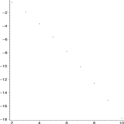
In figures 1 and 2 we give the frequency distribution of the four-point vertices for this theory, for $n=25$ (2.3$\;10^{32}$ diagrams) and $n=55$ (5.5$\;10^{91}$ diagrams).

Figure 1: Frequency distribution of the number of 4-point vertices in $\varphi^{3}+\varphi^{4}$ theory, for $n=25$. The solid line is the asymptotic estimate.

Figure 2: Frequency distribution of the number of 4-point vertices in $\varphi^{3}+\varphi^{4}$ theory, for $n=55$. The solid line is the asymptotic estimate.

Figure 3: Average fraction $\langle m\rangle/n$ for four-point vertices, as a function of $n$, in $\varphi^{3}+\varphi^{4}$ theory.

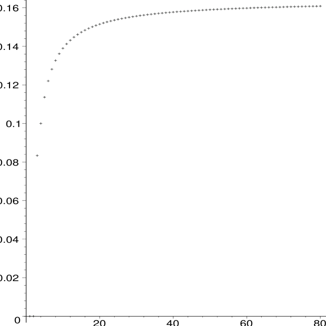
In figure 3, we give the actual value of the average number of four-point vertices as a fraction of $n$, for $1\leq n\leq 80$. The asymptotic value, 0.163986$\ldots$, is reached from below (as already evident from figures 1 and 2): the correction term appears to go as $1/4n$ in this range.

The second case of interest is a theory (like an effective theory, after tadpole and mass renormalization) where all types of vertices occur, that is, $\epsilon_{q}=1$ for all $q$. We have

$$W(\varphi)=e^{\varphi}-\varphi-1\;\;,$$ (23)

so that $f=\log(2)$, $f-W(f)=2\log(2)-1$, and $W^{\prime\prime}(f)=2$, and we have

$$\mu(q+1) = {(\log 2)^{q}\over q!(2\log 2-1)}\;\;,$$

$$\sigma(q+1)^{2} = \mu(q+1)\left[1+\mu-{(\log 2)^{q-2}\over 2(q-1)!}\right]\;\;.$$ (24)

In figure 4 we plot $\log\mu(q+1)$ for the first few values of $q$ for this theory. The values of $\sigma(q+1)^{2}$ follow quite closely: the numerical values of $\sigma(6)^{2}$ and $\mu(6)$ already differ by less than one percent.

Figure 4: $\log\mu(q)$ as a function of $q$ for a theory with all possible vertices.

4 Fine structure

In figure 5, we give the actual and asymptotic distribution of 3-point vertices in $\varphi^{3}+\varphi^{4}$ theory, for $n=35$.

Figure 5: Frequency distribution of 3-point vertices in $\varphi^{3}+\varphi^{4}$ theory, for $n=35$. The solid line is the coarse-grained asymptotic estimate.

Every Feynman diagram contains an even number of 3-point vertices. This follows of course from the topological sum rule for this theory:

$$m_{3}+2m_{4}=n-1$$ (25)

so that $m_{3}$ is either always even or always odd, depending on the parity of $n$. The asymptotic estimate does not reflect this; we shall now describe how also this ‘fine structure’ can be obtained, even in the asymptotic limit, as a consequence of the algebraic structure of the action. In order to be slightly more general, let us assume that there are two types of vertices present, one with $q+1$ legs and one with $p+1$ legs, and that we count the number of vertices of the first type. The Schwinger-Dyson equation now reads

$$\phi=x+z{\phi^{q}\over q!}+{\phi^{p}\over p!}$$ (26)

and the condition for the singularity reads

$$z{\phi^{q-1}\over(q-1)!}+{\phi^{p-1}\over(p-1)!}=1\;\;.$$ (27)

After having obtained $a(n;z)$, we can of course extract $b(n;m)$ by standard means:

$$b(n;m)={1\over 2i\pi}\int\limits_{z\sim 0}{a(n;z)\over z^{m+1}}dz\;\;,$$ (28)

where the integral is over an infinitesimal counterclockwise loop around $z=0$. Now notice that, for $z=0$, the singularity condition has not one but $p-1$ distinct solutions, which we shall denote by $\phi_{k}$:

$$\phi_{k}=(s!)^{1/s}\exp\left({2i\pi k\over s}\right)\;\;\;,\;\;\;k=0,1,2,\ldots,s-1\;\;\;,\;\;\;s\equiv p-1\;\;.$$ (29)

The corresponding values for $x=\phi_{k}-\phi_{k}^{p}/p!$ all have the same absolute value (at $z=0$, to be sure) and contribute equally to the asymptotic result. It therefore makes more sense to perform the integral not in terms of $z$ but in terms of the $\phi_{k}$, using Eq.(6). To this end, we write, for nonzero $z$, the singularity condition as

$$z={(q-1)!\over\phi^{q-1}}\left(1-{\phi^{s}\over s!}\right)={\mbox{``}H\mbox{''}(\phi^{s})\over\phi^{q-1}}$$ (30)

where by $\mbox{``}H\mbox{''}(\phi^{s})$ we denote an unspecified function of $\phi^{s}$. Inserting this expression for $z$ everywhere, we find

$$F(\phi,z)=\phi\mbox{``}H\mbox{''}(\phi^{s})\;\;\;,\;\;\;{\partial^{2}\over\partial\phi^{2}}F(\phi,z)={\mbox{``}H\mbox{''}(\phi^{s})\over\phi}\;\;\;,\;\;\;{dz\over d\phi}={\mbox{``}H\mbox{''}(\phi^{s})\over\phi^{q}}\;\;.$$ (31)

The above form for $b(n;m)$ is now a sum of loop integrals:

$$b(n;m) \sim \sum\limits_{k=0}^{s-1}\;{n!\over 2i\pi n^{3/2}}\;\int\limits_{\phi\sim\phi_{k}}\;{1\over z^{m+1}F(\phi,z)^{n}}\sqrt{{-F(\phi,z)\over 2\pi{\partial^{2}\over\partial\phi^{2}}F(\phi,z)}}{dz\over d\phi}\;d\phi$$ (32)

$$= \sum\limits_{k=0}^{s-1}\;\int\limits_{\phi\sim\phi_{k}}{1\over\phi^{n-m(q-1)}}\mbox{``}H\mbox{''}(\phi^{s})\;d\phi$$

$$= \int\limits_{\phi\sim\phi_{0}}{1\over\phi^{n-m(q-1)}}\mbox{``}H\mbox{''}(\phi^{s})\;d\phi$$

$$\hphantom{AAAAAAAA}\times\left(\sum\limits_{k=0}^{s-1}\exp\left({2i\pi k\over s}\right)^{1-n+m(q-1)}\right)\;\;,$$

owing to the $s$-fold symmetry of the unspecified function $\mbox{``}H\mbox{''}(\phi^{s})$. Now, the sum of the powers of the roots of unity in the above gives zero except when $1-n+m(q-1)$ happens to be a multiple of $s=p-1$, or in other words

$$m(q-1)+m^{\prime}(p-1)=n-1$$ (33)

for some $m^{\prime}$, which is again precisely the topological sum rule. In that case, we find exactly $s$ times the result from a single singular point, so that the normalization of the asymptotic distribution is preserved.

Two remarks are in order here. In the first place, the conclusion remains unchanged if other vertices are present, as long as these all have $ks+1$ legs ($k$ any integer larger than 1). If this algebraic symmetry is destroyed by the presence of another vertex type, there will in general be only one dominant singular point, and the vertex frequency distribution will not show any ‘quantisation’ anymore. In the second place, it is instructive to note that we arrive at the quantisation condition by working in the neighbourhood of $z=0$: once we move out to $z=1$, where the singular points are no longer symmetrically distributed, we move toward coarse-graining and a continuous distribution.

5 Vertex counting in QCD

We now turn to the more realistic case of QCD with both quarks and gluons. For simplicity we shall only consider a single quark flavour, as extensions to the case of more flavours is straightforward. We shall count the various vertices by assigning to the $q\bar{q}g$ vertex a weight $z_{q}$, and to the three- and four-gluon vertices weights $z_{3}$ and $z_{4}$, respectively. In any $1\to n$ amplitude we shall assign a factor $\bar{u}$ to an outgoing quark, a factor $v$ to an outgoing antiquark, and a factor $x$ to an outgoing gluon as before. The amplitude-generating function for an incoming quark is denoted by $\bar{\psi}$, that for an incoming antiquark by $\psi$, and that for an incoming gluon by $\phi$, again as before. The QCD Feynman rules now lead to the following coupled Schwinger-Dyson equations at the tree level:

$$\bar{\psi} = \bar{u}+z_{q}\bar{\psi}\phi\;\;\;,\;\;\;\psi=v+z_{q}\psi\phi\;\;,$$

$$\phi = x+{z_{3}\over 2}\phi^{2}+{z_{4}\over 6}\phi^{3}+z_{q}\bar{\psi}\psi\;\;,$$ (34)

We can rewrite this as an equation in terms of $\phi$ alone:

$$\phi=x+{z_{3}\over 2}\phi^{2}+{z_{4}\over 6}\phi^{3}+{z_{q}\xi\over(1-z_{q}\phi)^{2}}\;\;\;,\;\;\;\xi\equiv\bar{u}v\;\;.$$ (35)

The occurrence of the combination $\xi$ reflects fermion number conservation. The generating function $\phi$ is

$$\phi=\phi(x,\xi,\vec{z})=\sum\limits_{n_{g}\geq 0}\sum\limits_{n_{q}\geq 0}\sum\limits_{m_{3}\geq 0}\sum\limits_{m_{4}\geq 0}\sum\limits_{m_{q}\geq 0}c(n_{g},n_{q};m_{3},m_{4},m_{q}){x^{n_{g}}\over n_{g}!}{\xi^{n_{q}}\over n_{q}!^{2}}z_{3}^{m_{3}}z_{4}^{m_{4}}z_{q}^{m_{q}}$$ (36)

where $\vec{z}=(z_{3},z_{4},z_{q})$, and $c(n_{g},n_{q};m_{3},m_{4},m_{q})$ denotes the number of Feynman tree graphs with one incoming gluon, $n_{g}$ outgoing gluons, $n_{q}$ outgoing $q\bar{q}$ pairs, and precisely $m_{3}$ three-gluon vertices, $m_{4}$ four-gluon vertices and $m_{q}$ quark-gluon vertices. Again, explicit iteration of this equation gives $\phi$ as a multinomial in all its arguments, from which the number of graphs can be read off easily. Due to the larger number of counting variables the arriving at asymptotic estimates is more cumbersome in this case, but not qualitatively different. We have

$$x = F(\phi,\xi,\vec{z})$$ (37)

$$= \phi-{z_{3}\over 2}\phi^{2}-{z_{4}\over 6}\phi^{3}-{z_{q}\xi\over(1-z_{q}\phi)^{2}}\;\;,$$

and the large-$n_{g}$ behaviour is determined as before by requiring $dx/d\phi$ to vanish, which occurs when

$$\xi=\Xi(\phi,\vec{z})={1\over 2z_{q}^{2}}(1-z_{q}\phi)^{3}\left(1-z_{3}\phi-{z_{4}\over 2}\phi^{2}\right)\;\;.$$ (38)

For this value of $\xi$ we then have

$$X(\phi,\vec{z}) = F(\phi,\Xi(\phi,\vec{z}),\vec{z})$$ (39)

$$= {3\over 2}\phi-z_{3}\phi^{2}-{5\over 12}\phi^{3}+{1\over 2z_{q}}\left(1-z_{3}\phi-{z_{4}\over 2}\phi^{2}\right)^{2}\;\;.$$

By the same arguments as before, we find that the leading asymptotic behaviour is given by

$$g(n_{g},n_{q};\vec{z}) = \sum\limits_{m_{3,4,q}}c(n_{g},n_{q};m_{3},m_{4},m_{q})z_{3}^{m_{3}}z_{4}^{m_{4}}z_{q}^{m_{q}}$$ (40)

$$\sim {1\over X(\hat{\phi},\vec{z})^{n_{g}}\Xi(f,\vec{z})^{n_{q}}}\;\;,$$

where the saddle point $f$ is determined by

$$\left[{\partial\over\partial\phi}\left(\vphantom{A^{A}_{A}}n_{g}\log X(\phi,\vec{z})+n_{q}\log\Xi(\phi,\vec{z})\right)\right]_{\phi=f}\;\;.$$ (41)

From Eq.(40) it follows, by the probabilistic argument used before, that for $n_{g},n_{q}\to\infty$ the numbers $m_{3}$, $m_{4}$ and $m_{q}$ are all normally distributed. The mean values and variances are again found by taking the appropriate derivatives at $\vec{z}=(1,1,1)$. The saddle-point value is, in that case, given by

$$R(\rho,f)\equiv 6(1-\rho)-12f+3(1+\rho)f^{2}+(3-\rho)f^{3}=0\;\;,$$ (42)

where

$$n_{q}\equiv\rho N\;\;\;,\;\;\;N=n_{g}+2n_{q}\;\;.$$ (43)

The solution is given by

$$f = {1\over 3-\rho}\left\{-1-\rho-2b\sin\left[{1\over 3}\arcsin\left({2\over b^{3}}\left(\rho^{3}-9\rho^{2}+15\rho-23\right)\right)\right]\right\}\;\;,$$

$$b = \left(13-2\rho+\rho^{2}\right)^{1/2}\;\;.$$ (44)

The solution $f$ interpolates smoothly from $-1+\sqrt{3}\sim 0.732$ at $\rho=0$ to $-3/5+14/5\sin(\arcsin(282/343)/3)\sim 0.2854$ at $\rho=1/2$. The results for the mean values are

$$\langle m_{q}\rangle = N{6+3f^{2}-12\rho f^{2}-12f-18\rho f+3f^{3}+13\rho f^{3}+5\rho f^{4}\over(1-f)(-24f+5f^{3}+9f^{2}+6)}\;\;,$$

$$\langle m_{3}\rangle = N{2f(18f-12\rho f-6f^{3}+7\rho f^{3}-9f^{2}+9\rho f^{2}-6+6\rho)\over(-24f+5f^{3}+9f^{2}+6)(-2+f^{2}+2f)}\;\;,$$

$$\langle m_{4}\rangle = N{f^{2}(16f-8\rho f-5f^{3}+5\rho f^{3}-7f^{2}+5\rho f^{2}-6+6\rho)\over(-24f+5f^{3}+9f^{2}+6)(-2+f^{2}+2f)}\;\;.$$ (45)

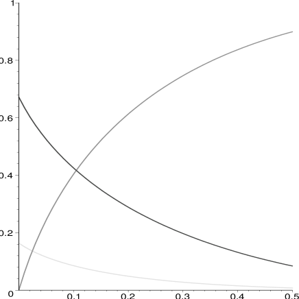
In figure 6 we give the results for the expectation values $\langle m_{j}\rangle/N$, with $j=q,3,4$.

Figure 6: Expected number of vertices of given type as a fraction of $N=n_{g}+2n_{q}$ in QCD with a single quark flavour. Along the horizontal axis we plot $\rho=n_{q}/N$. The rising curve is the result for the quark-gluon vertices, the falling curves are for the four-gluon vertex (lowest curve) and the three-gluon vertex (middle curve).

As a final check, note that the topological sum rule for the vertices in this case reads

$$m_{3}+2m_{4}+m_{q}=n_{g}+2n_{q}-2\sim N\;\;.$$ (46)

This is borne out by the numerical results, but also the analytic estimates (45) show that the combination

$$\langle m_{3}+2m_{4}+m_{q}-N\rangle$$

is precisely proportional to $R(f,\rho)$ and hence vanishes at the saddle point.

References

- [1] E. Argyres, R. Kleiss and C.G. Papadopoulos, Nucl. Phys. B391, 42, (1993)
- [2] M. Voloshin Multiparticle amplitudes at zero energy and momentum in scalar theory, Nucl. Phys. B383, 233, (1992)
- [3] P. Draggiotis and R. Kleiss, Counting tree diagrams:asymptotic results for QCD-like theories, Eur. Phys. J. C23, 701-706, (2002)