DESY 02-115
September 2002
Bulk and Brane Anomalies
In Six Dimensions

Abstract

We study anomalies of six-dimensional gauge theories compactified on orbifolds. In addition to the known bulk anomalies, brane anomalies appear on orbifold fixpoints in the case of chiral boundary conditions. At a fixpoint, where the bulk gauge group G is broken to a subgroup H, the non-abelian G-anomaly in the bulk reduces to a H-anomaly which depends in a simple manner on the chiral boundary conditions. We illustrate this mechanism by means of a SO(10) GUT model.

1 Introduction

The structure of the standard model of strong and electroweak interactions, its gauge group and field content, points towards an underlying unified theory (GUT) of all particles and interactions. The simplest GUT group which unifies the gauge interactions of the standard model is SU(5) [1]. With the present evidence for neutrino masses and mixings the larger gauge group SO(10) [2] appears particularly attractive. It contains SU(5) as well as the Pati-Salam group SU(4)$\times$SU(2)$\times$SU(2) [3] and flipped SU(5) [4] as subgroups.

The quest for unification with gravity points towards supersymmetry and higher dimensions. Orbifold compactifications [5] then provide a promising bridge to the four-dimensional world since they generically lead to chiral gauge theories as effective theories in lower dimensions. Hence, orbifold compactifications provide an attractive starting point for attempts to embed the standard model of particle physics into higher dimensional string and field theories.

Orbifold compactifications also allow to break the gauge symmetry of grand unified theories to the standard model gauge group in an attractive and simple manner. In particular, the breaking of the GUT symmetry automatically yields the required doublet-triplet splitting of Higgs fields [6]. Several SU(5) models have been constructed in five dimensions (5d) [6]-[9], whereas six dimensions are required for the breaking of SO(10) [10, 11]. Global anomaly cancellation [12] or extended supersymmetry [13] in 6d can also be used to explain the number of quark-lepton generations.

In general, orbifold compactifications lead to anomalies at orbifold fixpoints. So far, this has been studied for U(1) symmetries in 5d theories [14]-[17] and for 10d heterotic orbifolds [18] , where no bulk anomalies exist. The cancellation of the brane anomalies at orbifold fixpoints is crucial for the consistency of the orbifold compactification and the field content of the theory.

In the present paper we investigate anomalies in orbifold compactifications of 6d theories. This is motivated by recently proposed supersymmetric 6d GUT models. Contrary to five dimensions, bulk anomalies exist in six dimensions for N=1 supersymmetry, and the question arises how brane and bulk anomalies are related.

It turns out that Fujikawa’s method of calculating anomalies is particularly well suited to study this question. In section 2 we shall explicitly calculate the U(1) anomaly of a 6d Weyl fermion on the orbifold $M=\mathcal{R}^{4}\times T^{2}/Z_{2}$ and compare the result with the anomaly in flat space $M=\mathcal{R}^{6}$ and on the torus, $M=\mathcal{R}^{4}\times T^{2}$. In section 3 we extend this result to non-abelian anomalies and determine the general connection between the brane anomalies and the chiral boundary conditions at orbifold fixpoints. This pattern will be illustrated in more detail in section 4 by means of the SO(10) GUT model proposed in [19]. Our results are summarized in section 5, and some useful formulae are collected in the appendices.

2 The abelian anomaly in six dimensions

Consider a Weyl fermion $\psi$ with U(1) gauge interaction in six dimensions, which is described by the lagrangian

$${\cal L}=\bar{\psi}(z)i\Gamma^{M}D_{M}\psi(z)\;.$$ (1)

Here $D_{M}=\partial_{M}+A_{M}$, $M=1\ldots 6$, is the covariant derivative with field strength $F_{MN}=[D_{M},D_{N}]$. The 6d Weyl fermion is composed of two 4d Weyl fermions with opposite 4d chirality, $\psi=(\psi_{L},\psi_{R})$, with $\gamma_{5}\psi_{L}=-\psi_{L}$ and $\gamma_{5}\psi_{R}=\psi_{R}$; $\psi$ has negative 6d chirality, i.e. $\Gamma_{7}\psi=-\psi$, where $\Gamma_{7}$ = diag($\gamma_{5},-\gamma_{5}$).

Naive dimensional reduction to five dimensions yields a U(1) gauge theory with a Dirac fermion, $\chi=\psi_{L}+\psi_{R}$, with U(1) gauge interaction,

$${\cal L}=\bar{\chi}(z)i\gamma^{M}D_{M}\chi(z)\;,$$ (2)

where $\gamma^{M}$, $M=1\ldots 5$, are the usual 4d $\gamma$-matrices. This model has been discussed in the literature in connection with anomalies arising on the orbifold $S^{1}/Z_{2}$ [14]-[17].

We now consider the compactification of the 6d theory on the orbifold $M=\mathcal{R}^{4}\times T^{2}/Z_{2}$. The two elements of the group $Z_{2}$ are the identity and the reflection at one point on the torus $T^{2}$, e.g. $y\rightarrow-y$, where $y=(z^{5},z^{6})$. The orbifold $T^{2}/Z_{2}$ has four fixpoints, $y_{1}=(0,0)$, $y_{2}=(\pi R_{5},0)$, $y_{3}=(0,\pi R_{6})$ and $y_{4}=(\pi R_{5},\pi R_{6})$, which correspond to the four corners of a ‘pillow’. Here $R_{5},R_{6}$ are the radii of the torus in the $z^{5}$ and $z^{6}$ direction respectively. For the fermion $\psi$ we impose chiral boundary conditions,

$$\psi_{L}(x,y)=\psi_{L}(x,-y)\;,\quad\psi_{R}(x,y)=-\psi_{R}(x,-y)\;,$$ (3)

where $x$ denotes the coordinates of flat 4d Minkowski space. In terms of the complete system of mode functions (cf. appendix C), the fermions $\psi_{L}$ and $\psi_{R}$ can be expanded as

$$\psi_{L}(x,y)=\sum_{mn}\psi_{L+}^{mn}(x)\xi^{mn}_{+}(y)\;,\quad\psi_{R}(x,y)=\sum_{mn}\psi_{R-}^{mn}(x)\xi^{mn}_{-}(y)\;.$$ (4)

Invariance of the lagrangian under the $Z_{2}$ symmetry requires for the background gauge field,

$$A_{\mu}(x,y)=A_{\mu}(x,-y)\;,\quad A_{5,6}(x,y)=-A_{5,6}(x,-y)\;.$$ (5)

Note, that $A_{5,6}$ vanishes at the fixpoints $y_{i}$, $i=1\ldots 4$.

The effective action $\Gamma[A]$, which is defined by

$$e^{i\Gamma[A]}=\int D\psi D\bar{\psi}\exp\left(i\int d^{6}z{\cal L}\right)\;,$$ (6)

transforms under infinitesimal gauge transformations $\delta_{v}A_{M}=\partial_{M}v$ as

$$\delta_{v}\Gamma[A]=\int d^{6}z\,\left(\partial^{M}\left[v(z)\,J_{M}(z)\right]-v(z)\partial^{M}\!J_{M}(z)\right)\;,$$ (7)

where $J_{M}(z)=\delta\Gamma[A]/\delta A^{M}(z)$ is the U(1) current. We have kept for generality the boundary term due to the partial integration. In the case of singular currents and manifolds with boundaries, like in the orbifold case, a contribution from the boundary can survive [20]. Due to the non-invariance of the measure $D\psi D\bar{\psi}$ gauge invariance is spoiled [21],

$$\delta_{v}\Gamma[A]=-\int d^{6}z\,v(z){\cal A}(z)\;.$$ (8)

For vanishing boundary term the divergence of the current is then given by the anomaly [22],

$$\partial^{M}\!J_{M}(z)={\cal A}(z)\;,$$ (9)

which can be expressed as a trace over modes of $\psi$ and $\bar{\psi}$, respectively [21].

Let $\phi_{n}$ be a complete set of eigenfunctions $\phi_{n}$ of the hermitian operator ${\hbox to0.0pt{\hbox{$\mskip 3.0mu/$}\hss}D}^{2}=(\Gamma^{M}D_{M})^{2}$ with eigenvalues $\lambda_{n}^{2}$, i.e. ${\hbox to0.0pt{\hbox{$\mskip 3.0mu/$}\hss}D}^{2}\phi_{n}=\lambda_{n}^{2}\phi_{n}$. A left-handed 6d Weyl fermion $\psi$ can be expanded into eigenfunctions of ${\hbox to0.0pt{\hbox{$\mskip 3.0mu/$}\hss}D}^{2}$ and $(1-\Gamma_{7})/2$. Correspondingly, $\bar{\psi}$ is right-handed and can be expanded in eigenfunctions of ${\hbox to0.0pt{\hbox{$\mskip 3.0mu/$}\hss}D}^{2}$ and $(1+\Gamma_{7})/2$. The anomaly is then given by the difference of sums over left-handed and right-handed modes, respectively [21, 23, 24],

$${\cal A}(z)=\lim_{\Lambda\to\infty}\sum_{n}\left(\phi_{n}^{\dagger}(z){1-\Gamma_{7}\over 2}\phi_{n}(z)-\phi_{n}^{\dagger}(z){1+\Gamma_{7}\over 2}\phi_{n}(z)\right)e^{-\lambda_{n}^{2}/\Lambda^{2}}\;,$$ (10)

where the sum has been regularized by the ultraviolet cutoff $\Lambda$. Choosing plane waves as eigenfunctions in flat space, one obtains [23],

$${\cal A}(z) = -\lim_{\Lambda\to\infty}{\rm Tr}\int{d^{6}k\over(2\pi)^{6}}\Gamma_{7}e^{ikz}e^{-{\hbox to0.0pt{\hbox{$\mskip 1.0mu/$}\hss}D}^{2}/\Lambda^{2}}e^{-ikz}$$ (11)

$$= -\lim_{\Lambda\to\infty}{\rm Tr}\int{d^{6}k\over(2\pi)^{6}}\Gamma_{7}\exp\left({(k+iD)^{2}\over\Lambda^{2}}-{1\over 4\Lambda^{2}}[\Gamma^{M},\Gamma^{N}]F_{MN}\right)$$

$$= -\lim_{\Lambda\to\infty}{1\over 3!}{\rm Tr}\ \Gamma_{7}\left({-1\over 4\Lambda^{2}}[\Gamma^{M},\Gamma^{N}]F_{MN}\right)^{3}\Lambda^{6}\,\int{d^{6}k\over(2\pi)^{6}}e^{k^{2}}$$

$$= -\,{i^{3}\over 3!(4\pi)^{3}}\epsilon^{MNPQRS}F_{MN}F_{PQ}F_{RS}\;.$$

Here ${\rm Tr}$ denotes the trace over Dirac matrices in 6d, and after Wick rotation to Euclidean space the metric is $\eta_{MN}^{E}=-\delta_{MN}$.

If two of the six dimensions are compactified on a torus one can choose as eigenfunctions the product of 4d plane waves with the orthonormal modes $\xi^{mn}_{\pm}$ on $T^{2}$ (cf. appendix C). The sum over all modes then reads

$${\rm Tr}\int{d^{4}k\over(2\pi)^{4}}e^{k^{2}/\Lambda^{2}}\sum_{mn}e^{-{M_{m}^{2}+M_{n}^{2}\over\Lambda^{2}}}\left({\xi_{+}^{mn}}^{2}(y)+{\xi_{-}^{mn}}^{2}(y)\right)\;,$$ (12)

which, in the limit $\Lambda R_{5,6}\rightarrow\infty$, becomes the 6d sum of flat space, i.e. $\int d^{6}k/(2\pi)^{6}\exp{(k^{2}/\Lambda^{2})}$. Hence, the abelian anomaly on $M=\mathcal{R}^{4}\times T^{2}$ is identical to the one in flat space.

Consider now compactification on the orbifold $M=\mathcal{R}^{4}\times T^{2}/Z_{2}$. In this case the physical space corresponds to the pillow with corners $y_{1}=(0,0)$, $y_{2}=(\pi R_{5},0)$, $y_{3}=(0,\pi R_{6})$ and $y_{4}=(\pi R_{5},\pi R_{6})$, with half the volume of the torus. The variation of the action then reads

$$\delta_{v}\Gamma[A] = -\int d^{4}x\,\int_{T^{2}/Z_{2}}\!d^{2}y\,v(x,y)\partial^{M}\!J_{M}(x,y)$$ (13)

$$= -\int d^{4}x\,\int_{T^{2}/Z_{2}}\!d^{2}y\,v(x,y){\cal A}(x,y)\;$$ (14)

$$= -\int d^{4}x\,\int_{T^{2}}\!d^{2}y\,v(x,y){\cal A}_{cov}(x,y)\;,$$ (15)

where in the last line we have extended the integral to the covering space $T^{2}$. In this way we can resort to the trick of using mode functions on $T^{2}$ and compare more directly the result with the torus case. For the relation between ${\cal A}$ and ${\cal A}_{cov}$ see appendix D.

Another difference is that on the orbifold the chiral boundary conditions (3) have to be taken into account in the sum over the modes of $\psi$ and $\bar{\psi}$. This can be done by means of the projection operators

$${1\pm\Gamma_{7}\over 2}\hat{P}_{L(R)}\;,$$ (16)

where the 4d chirality operator acting on 6d spinors is defined as

$$\hat{P}_{L(R)}=\left(\begin{tabular}[]{cc}$P_{L(R)}$&0\\ 0&$P_{L(R)}$\end{tabular}\right)\;,$$ (19)

and $P_{L(R)}=(1\mp\gamma_{5})/2$ is the usual 4d chiral projector. The operators in eq. (16) single out the components $\psi_{L(R)}$ of the 6d Weyl spinor $\psi$. For the anomaly one then obtains (cf. (11)),

$${\cal A}_{cov}(x,y) = \lim_{\Lambda\to\infty}{\rm Tr}\int{d^{4}k\over(2\pi)^{4}}e^{ikx}\sum_{mn}e^{-{\hbox to0.0pt{\hbox{$\mskip 1.0mu/$}\hss}D}^{2}/\Lambda^{2}}e^{-ikx}$$

$$\hskip 17.07182pt\times\left[{1-\Gamma_{7}\over 2}\left(\hat{P}_{L}{\xi_{+}^{mn}}^{2}(y)+\hat{P}_{R}{\xi_{-}^{mn}}^{2}(y)\right)\right.$$

$$\hskip 28.45274pt\left.-{1+\Gamma_{7}\over 2}\left(\hat{P}_{R}{\xi_{+}^{mn}}^{2}(y)+\hat{P}_{L}{\xi_{-}^{mn}}^{2}(y)\right)\right],$$

which is conveniently expressed as

$${\cal A}_{cov}(x,y) = -{1\over 2}\lim_{\Lambda\to\infty}{\rm Tr}\int{d^{4}k\over(2\pi)^{4}}e^{k^{2}/\Lambda^{2}}\sum_{mn}e^{-{M_{m}^{2}+M_{n}^{2}\over\Lambda^{2}}}\exp{\left({-1\over 4\Lambda^{2}}[\Gamma^{M},\Gamma^{N}]F_{MN}\right)}$$

$$\hskip 34.14322pt\times\left[\Gamma_{7}\left({\xi_{+}^{mn}}^{2}(y)+{\xi_{-}^{mn}}^{2}(y)\right)+\left(\hat{P}_{R}-\hat{P}_{L}\right)\left({\xi_{+}^{mn}}^{2}(y)-{\xi_{-}^{mn}}^{2}(y)\right)\right]\ .$$

The term proportional to $(\xi_{+}^{2}+\xi_{-}^{2})$ is identical to the anomaly on the torus, up to a factor $1/2$. Hence, we obtain on the covering space half the bulk anomaly of flat space. This is plausible since we have projected out half of the modes. In fact we can write the torus wavefunction as a sum of two orbifold wavefunctions with opposite parities and recover the result of eq. (12). Remember anyway that the orbifold bulk anomaly on the physical space is larger by a factor 2 (cf. appendix D), so that locally one cannot distinguish the global properties of the space.

On the other hand, the sum over the difference of modes, $(\xi_{+}^{2}-\xi_{-}^{2})$, is finite (cf. appendix C), and independent of the cut-off,

$$\sum_{mn}\left({\xi_{+}^{mn}}^{2}(y)-{\xi_{-}^{mn}}^{2}(y)\right)=\delta_{O}(y)\;.$$ (22)

Correspondingly, taking the limit $\Lambda\rightarrow\infty$, the term proportional to ${\rm Tr}\left(\hat{P}_{R}-\hat{P}_{L}\right)\left([\Gamma^{M},\Gamma^{N}]F_{MN}\right)^{3}$ vanishes, whereas a term ${\rm Tr}\left(\hat{P}_{R}-\hat{P}_{L}\right)\left([\Gamma^{M},\Gamma^{N}]F_{MN}\right)^{2}$ survives, proportional to the 4d anomaly. Combining both terms we finally obtain for the anomaly,

$${\cal A}_{cov}(x,y)=-\,{1\over 2}{i^{3}\over 3!(4\pi)^{3}}\epsilon^{MNPQRS}F_{MN}F_{PQ}F_{RS}+{i^{2}\over 2!(4\pi)^{2}}\delta_{O}(y)\epsilon^{\mu\nu\rho\sigma}F_{\mu\nu}F_{\rho\sigma}\;.$$ (23)

As described in the appendix D, the anomaly on the physical space $T^{2}/Z_{2}$ reads then

$${\cal A}(x,y)=-\,{i^{3}\over 3!(4\pi)^{3}}\epsilon^{MNPQRS}F_{MN}F_{PQ}F_{RS}+{i^{2}\over 2!(4\pi)^{2}}\delta_{O}(y)\epsilon^{\mu\nu\rho\sigma}F_{\mu\nu}F_{\rho\sigma}\;.$$ (24)

The interpretation of this result is obvious: the first term is the usual 6d bulk anomaly, and the second term, generated by the chiral boundary conditions at the orbifold fixpoints, is a localized 4d anomaly. Note that the sum of the 4d anomalies at the fixpoints equals the 4d anomaly of the zero mode $\psi_{L}^{00}$. In fact the contributions of the massive modes to the integrated anomaly compensate each other for every Kaluza-Klein level $(m,n)$. In the effective 4d low energy theory therefore only the contribution of the zero modes survives, if the bulk anomaly vanishes.

For comparison, it is instructive to compute also the abelian anomaly in five dimensions, on the orbifold $M=\mathcal{R}^{4}\times S^{1}/Z_{2}$. The two fixpoints are $y_{1}=0$ and $y_{2}=\pi R_{5}$, with $y=z^{5}$. The chiral boundary conditions are again given by eq. (3). Fermions are now four-component spinors, $\chi=\psi_{L}+\psi_{R}$, and left- and right-handed spinors can be expanded in terms of $\xi^{m}_{+}$ and $\xi^{m}_{-}$, respectively (cf. appendix C). The trace formula (2) for the 6d anomaly then becomes

$${\cal A}_{cov}(x,y) = \lim_{\Lambda\to\infty}{\rm Tr}\int{d^{4}k\over(2\pi)^{4}}e^{ikx}\sum_{m}e^{-{\hbox to0.0pt{\hbox{$\mskip 1.0mu/$}\hss}D}^{2}/\Lambda^{2}}e^{-ikx}$$ (25)

$$\hskip 34.14322pt\times\left[\left(P_{L}{\xi_{+}^{m}}^{2}(y)+P_{R}{\xi_{-}^{m}}^{2}(y)\right)-\left(P_{R}{\xi_{+}^{m}}^{2}(y)+P_{L}{\xi_{-}^{m}}^{2}(y)\right)\right]\;,$$

which yields

$${\cal A}_{cov}(x,y) = -\lim_{\Lambda\to\infty}{\rm Tr}\int{d^{4}k\over(2\pi)^{4}}e^{k^{2}/\Lambda^{2}}\sum_{m}e^{-{M_{m}^{2}\over\Lambda^{2}}}\exp{\left({-1\over 4\Lambda^{2}}[\Gamma^{M},\Gamma^{N}]F_{MN}\right)}$$ (26)

$$\hskip 73.97733pt\times\left[\gamma_{5}\left({\xi_{+}^{m}}^{2}(y)-{\xi_{-}^{m}}^{2}(y)\right)\right]\ .$$

As on the torus, the sum over the differences of modes, $(\xi_{+}^{2}-\xi_{-}^{2})$, is finite, and one finally obtains

$${\cal A}_{cov}(x,y)={\cal A}(x,y)={1\over 2}\left(\delta(y)+\delta(y-\pi R^{5})\right){i^{2}\over 2!(4\pi)^{2}}\epsilon^{\mu\nu\rho\sigma}F_{\mu\nu}F_{\rho\sigma}\;.$$ (27)

This result has previously been obtained [14] by direct evaluation of the divergence of the 5d U(1) current, using the known 4d anomaly, and also by means of Fujikawa’s method [16].

3 The non-abelian anomaly

The abelian anomaly (24) is most conveniently written as differential form. With

$$A=A_{M}dz^{M}\;,\quad F=dA={1\over 2}F_{MN}dz^{M}dz^{N}\;,$$ (28)

one obtains for the 6-form $\hat{{\cal A}}={\cal A}(z)dz^{1}\ldots dz^{6}$,

$$\hat{{\cal A}}=-\,{i^{3}\over(2\pi)^{3}}F^{3}+\delta_{O}(y)dz^{5}dz^{6}{i^{2}\over(2\pi)^{2}}F^{2}\;,$$ (29)

where wedge products are understood.

Consider now a 6d Weyl fermion $\psi$ in a non-abelian background field which is an element of the Lie algebra, i.e. $D_{M}=\partial_{M}+A_{M}$ and $A_{M}=iA_{M}^{a}T^{a}$, where $T^{a}$ are the generators of the group G. Field strength and gauge variation are now

$$F=dA+A^{2}\;,\quad\delta_{v}A=dv+[A,v]\;,$$ (30)

where $v=iv^{a}T^{a}$. The variation of the effective action, neglecting the boundary term, is given by

$$\delta_{v}\Gamma[A]=-\int d^{6}z\,v^{a}(z)\left({\cal A}^{a}(z)+\Delta_{WZ}^{a}(z)\right)\;.$$ (31)

The non-abelian anomaly ${\cal A}^{a}+\Delta_{WZ}^{a}$ satisfies the Wess-Zumino consistency conditions [25]. It differs from the covariant anomaly ${\cal A}^{a}$ by $\Delta_{WZ}^{a}$, a local polynomial in the gauge field [24]. Since we are only interested in the question of anomaly cancellation, we can ignore this difference and consider just the covariant anomaly which is again given by a trace formula [24],

$${\cal A}^{a}(z)=\lim_{\Lambda\to\infty}\sum_{n}\left(\phi_{n}^{\dagger}(z)T^{a}{1-\Gamma_{7}\over 2}\phi_{n}(z)-\phi_{n}^{\dagger}(z)T^{a}{1+\Gamma_{7}\over 2}\phi_{n}(z)\right)e^{-\lambda_{n}^{2}/\Lambda^{2}}\;.$$ (32)

A calculation completely analogous to the one in section 2 then yields for the non-abelian anomaly on the orbifold $\mathcal{R}^{4}\times T^{2}/Z_{2}$,

$$\hat{{\cal A}}^{a}(x,y)=-\;{i^{3}\over(2\pi)^{3}}{\rm tr}\left(T^{a}F^{3}\right)\;+\;\delta_{O}(y)dz^{5}dz^{6}{i^{2}\over(2\pi)^{2}}{\rm tr}\left(T^{a}F^{2}\right)\;,$$ (33)

where ${\rm tr}$ denotes the trace over the fermion representation of the group G.

Boundary conditions at orbifold fixpoints can be used to break the group G to a symmetric subgroup H. This is achieved by means of an automorphism of the Lie algebra, characterized by a parity operator $P$, with $P^{2}=I$. For the gauge field $A$, the corresponding boundary conditions read

$$PA_{\mu}(x,-y)P^{-1} = +A_{\mu}(x,y)\;,\quad PA_{5,6}(x,-y)P^{-1}=-A_{5,6}(x,y)\;.$$ (34)

Note, that $P$ acts differently on the generators $T^{\tilde{a}}$ of $H$ and $T^{\hat{a}}$ of $G/H$,

$$PT^{\tilde{a}}P^{-1}=+T^{\tilde{a}}\;,\quad PT^{\hat{a}}P^{-1} = -T^{\hat{a}}\;,$$ (35)

allowing zero modes only for $A^{\tilde{a}}_{\mu}$ and $A^{\hat{a}}_{5,6}$. Also the 6d gauge transformations are restricted to those with $\partial_{\mu}v^{\hat{a}}(x,0)=0\,,\partial_{5,6}v^{\tilde{a}}(x,0)=0$. Hence, only the local symmetry corresponding to $H$ is present at the orbifold fixed point.

The 6d Weyl fermion, $\psi=(\psi_{L},\psi_{R})$, splits into two, in general reducible, representations of H, $\psi=(\psi_{1},\psi_{2})$, which have positive and negative parity, respectively,

$$P\psi_{1}(x,y)=+\psi_{1}(x,y)\;,\quad P\psi_{2}(x,y)=-\psi_{2}(x,y)\;.$$ (36)

The chiral boundary condition (3) then becomes

$$P\psi_{L1}(x,-y) = +\psi_{L1}(x,y)\;,\quad P\psi_{L2}(x,-y)=-\psi_{L2}(x,y)\;,$$ (37)

$$P\psi_{R1}(x,-y) = -\psi_{R1}(x,y)\;,\quad P\psi_{R2}(x,-y)=+\psi_{R2}(x,y)\;.$$ (38)

These boundary conditions allow only two 4d zero modes, one left- and one right-handed fermion in two different representations of H, which can be characterized by the projection operators $P_{1}=(1+P)/2$ and $P_{2}=(1-P)/2$.

We can now again calculate the non-abelian anomaly on the orbifold with the new boundary conditions which break G to H. The anomaly is given by the same expression as (2) except for the mode sum which has to be replaced by

$$\sum_{mn}e^{-{M_{m}^{2}+M_{n}^{2}\over\Lambda^{2}}}\left\{{1-\Gamma_{7}\over 2}\left[\left(\hat{P}_{L}P_{1}+\hat{P}_{R}P_{2}\right){\xi_{+}^{mn}}^{2}(y)+\left(\hat{P}_{L}P_{2}+\hat{P}_{R}P_{1}\right){\xi_{-}^{mn}}^{2}(y)\right]\right.$$

$$\hskip 22.76228pt\left.-{1+\Gamma_{7}\over 2}\left[\left(\hat{P}_{R}P_{1}+\hat{P}_{L}P_{2}\right){\xi_{+}^{mn}}^{2}(y)+\left(\hat{P}_{R}P_{2}+\hat{P}_{L}P_{1}\right){\xi_{-}^{mn}}^{2}(y)\right]\right\}\;.$$ (39)

This expression can again conveniently be written in the form of eq. (2), with the mode sum,

$$\sum_{mn}e^{-{M_{m}^{2}+M_{n}^{2}\over\Lambda^{2}}}\left\{\Gamma_{7}\left({\xi_{+}^{mn}}^{2}(y)+{\xi_{-}^{mn}}^{2}(y)\right)\right.$$

$$\hskip 42.67912pt\left.+\left(\hat{P}_{R}-\hat{P}_{L}\right)\left(P_{1}-P_{2}\right)\left({\xi_{+}^{mn}}^{2}(y)-{\xi_{-}^{mn}}^{2}(y)\right)\right\}\;.$$ (40)

Note that, as before, $\hat{P}_{R}-\hat{P}_{L}=$ diag$(\gamma_{5},\gamma_{5})$, while $P_{1}-P_{2}=P$.

The final expression for the anomaly then reads

$$\hat{{\cal A}}^{a}(x,y) = -\,{i^{3}\over(2\pi)^{3}}{\rm tr}\left(T^{a}F^{3}\right)+\delta_{O}(y)dz^{5}dz^{6}{i^{2}\over(2\pi)^{2}}{\rm tr}\left((P_{1}-P_{2})T^{a}F^{2}\right)$$ (41)

$$= -\,{i^{3}\over(2\pi)^{3}}{\rm tr}\left(T^{a}F^{3}\right)+\delta_{O}(y)dz^{5}dz^{6}{i^{2}\over(2\pi)^{2}}{\rm tr}\left(PT^{a}F^{2}\right)\;.$$ (42)

The only difference with respect to eq. (33), the anomaly in the case without symmetry breaking, is the appearance of projection operators, and therefore of the parity operator $P$, in the second term. At the fixpoint, the group G is broken to the subgroup H. It is therefore consistent to have in the fixpoint term of the anomaly projection operators $P_{1}$ and $P_{2}$ for the two different representations of H. The relative sign is different, since the chiral boundary conditions (37), (38) associate a 4d left-handed fermion with $P_{1}$ and a 4d right-handed fermion with $P_{2}$.

At the fixpoint only the gauge group $H$ can act, and the gauge variation $\partial_{\mu}v^{\hat{a}}$ for the coset $G/H$ vanishes there. Correspondingly, for the localized anomaly the trace ${\rm tr}\left(PT^{\hat{a}}F^{2}\right)$ vanishes for any generator $T^{\hat{a}}$ belonging to the coset $G/H$, since we have

$${\rm tr}\left(PT^{\hat{a}}F^{2}\right)=-{\rm tr}\left(PT^{\hat{a}}F^{2}\right)=0\;,$$ (43)

from $PT^{\hat{a}}=-T^{\hat{a}}P$ and $PF^{2}=F^{2}P$.

Similarly, also the bulk anomaly at the fixpoint is non-zero only for generators $T^{\tilde{a}}$ belonging to $H$. In fact, there the non-vanishing fields are $F^{\tilde{a}}_{\mu\nu},F^{\tilde{a}}_{56}$ and $F^{\hat{a}}_{\mu 5},F^{\hat{a}}_{\mu 6}$. Hence, the only completely antisymmetric terms are of the type

$${\rm tr}\left(T^{a}T^{\tilde{a}}T^{\tilde{a}^{\prime}}T^{\tilde{a}^{\prime\prime}}\right)\epsilon^{\mu\nu\rho\sigma}F^{\tilde{a}}_{\mu\nu}F^{\tilde{a}^{\prime}}_{\rho\sigma}F^{\tilde{a}^{\prime\prime}}_{56}\;,$$ (44)

corresponding to the bulk $H$ anomaly term, and the mixed piece

$${\rm tr}\left(T^{a}T^{\tilde{a}}T^{\hat{a}}T^{\hat{a}^{\prime}}\right)\epsilon^{\mu\nu\rho\sigma}F^{\tilde{a}}_{\mu\nu}F^{\hat{a}}_{\rho 5}F^{\hat{a}^{\prime}}_{\sigma 6}\;.$$ (45)

Both group traces vanish identically for generators $T^{a}$ belonging to $G/H$, since they contain an odd number of generators of $G/H$, with negative parity.

So at the fixed point the non-abelian anomaly is restricted to the subgroup $H$ of the original group $G$. But while the brane anomaly contains only $F^{\tilde{a}}_{\mu\nu}$ and reduces automatically to the anomaly of the unbroken subgroup $H$, in the bulk piece an additional mixed term (45) survives.

If we integrate over the compact space, we obtain two contributions that affect the low energy effective 4d theory: on one side part of the bulk anomaly survives and gives rise to derivative interactions between the zero modes and the Kaluza-Klein tower of the gauge field, on the other hand the localized piece reduces to the 4d anomaly of the zero modes, as in the case of the abelian anomaly.

Therefore, in order to have a viable 4d low energy theory, we need to impose the vanishing of the irreducible bulk anomaly and also require an anomaly-free configuration for the zero modes.

4 An SO(10) GUT model

We are now ready to consider a more interesting example, the SO(10) GUT model proposed in ref. [19]. We consider SO(10) Yang-Mills theory in 6d with N=1 supersymmetry. The gauge fields $A_{M}$ and the gauginos $\lambda_{1}$, $\lambda_{2}$ are conveniently grouped into vector and chiral multiplets of the unbroken N=1 supersymmetry in 4d,

$$A=(A_{\mu},\lambda_{1})\;,\quad\Sigma=(A_{5,6},\lambda_{2})\;.$$ (46)

Here $A$ and $\Sigma$ are matrices in the adjoint representation of SO(10).

Symmetry breaking is achieved by compactification on the orbifold $T^{2}/(Z_{2}^{I}\times Z_{2}^{PS}\times Z_{2}^{GG})$. The discrete symmetries $Z_{2}$ break the extended supersymmetry. They also break the SO(10) gauge group down to the subgroups SO(10), G_PS=SU(4)$\times$SU(2)$\times$SU(2), G_GG=SU(5)$\times$U(1)_X and G_fl=SU(5)${}^{\prime}\times$U(1)^′, at the four fixpoints $y_{1}=y_{O}=(0,0)$, $y_{2}=y_{PS}=(\pi R_{5}/2,0)$, $y_{3}=y_{GG}=(0,\pi R_{6}/2)$ and $y_{4}=y_{fl}=(\pi R_{5}/2,\pi R_{6}/2)$,

$$P_{I}A(x,y_{O}-y)P_{I}^{-1} = \eta_{I}A(x,y_{O}+y)\;,$$ (47)

$$P_{PS}A(x,y_{PS}-y)P_{PS}^{-1} = \eta_{PS}A(x,y_{PS}+y)\;,$$ (48)

$$P_{GG}A(x,y_{GG}-y)P_{GG}^{-1} = \eta_{GG}A(x,y_{GG}+y)\;,$$ (49)

$$P_{fl}A(x,y_{fl}-y)P_{fl}^{-1} = \eta_{fl}A(x,y_{fl}+y)\;.$$ (50)

Here $P_{I}=I$, the matrices $P_{PS}$ and $P_{GG}$ are given in the appendix, and $P_{fl}=P_{GG}P_{PS}$, with $\eta_{fl}=\eta_{GG}\eta_{PS}$. The parities are chosen as $\eta_{I}=\eta_{PS}=\eta_{GG}=+1$. The extended supersymmetry is broken by choosing in the corresponding equations for $\Sigma$ all parities $\eta_{i}=-1$.

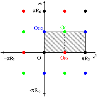
Figure 1: Orbifold $T^{2}/(Z_{2}^{I}\times Z_{2}^{PS}\times Z_{2}^{GG})$ with the fixpoints $O$, $O_{PS}$, $O_{GG}$, and $O_{fl}$.

Figure 1 shows the four fixpoints, together with their three images each, on the covering space $T^{2}$, with $z^{5}\in(-\pi R_{5},\pi R_{5}]$ and $z^{6}\in(-\pi R_{6},\pi R_{6}]$. The physical region is obtained by folding the shaded region along the dotted line and gluing the edges. The result is a ‘pillow’ with the four fixpoints as corners. The unbroken gauge group of the effective 4d theory is given by the intersection of the SO(10) subgroups at the fixpoints. In this way one obtains the standard model group with an additional U(1) factor, G${}_{SM^{\prime}}$= SU(3)$\times$SU(2)$\times$U(1)${}_{Y}\times$U(1)_X. The zero modes of the vector multiplet $A$ form the gauge fields of G${}_{SM^{\prime}}$.

Matter and Higgs fields have been introduced motivated by the coset spaces E₈/(SO(10)$\times$H_F) where H_F is a subgroup of SU(3)$\times$U(1) [26]-[29], which have previously been discussed in connection with 4d supersymmetric $\sigma$-models. In the case H${}_{F}=$SU(3)$\times$U(1) the complex structure, and the corresponding representation of chiral multiplets is unique,

$$\Omega=({\bf 16},{\bf 3})_{1}+({\bf 16^{*}},{\bf 1})_{3}+({\bf 10},{\bf 3^{*}})_{2}+({\bf 1},{\bf 3})_{4}\;.$$ (51)

The SO(10) representations can in principle account for three quark-lepton generations, contained in the three 16’s of SO(10), one mirror generation 16^∗ and Higgs fields in the 10’s. For bulk fields, however, only split multiplets appear as zero modes in the effective 4d theory.

It is remarkable that the requirement of SO(10) bulk anomaly cancellation determines the distribution of the SO(10) multiplets between bulk and branes. The vector multiplet is a 45-plet of SO(10) which has a 6d anomaly. The irreducible anomalies of fermions in the adjoint, vector and spinor representations are related by (cf. [30]),

$$a_{(4)}({\bf 45})=2a_{(4)}({\bf 10})\;,\quad a_{(4)}({\bf 16})=a_{(4)}({\bf 16^{*}})=-a_{(4)}({\bf 10})\;.$$ (52)

Since fermions in vector and hypermultiplets have opposite chirality, the irreducible anomaly of the vector multiplet can be canceled by adding two 10-plet hypermultiplets, $H_{1}$ and $H_{2}$. The complex structure (51) then requires all three 10-plets, and, consequently, also the 16^∗-plet to be bulk fields whereas the three 16’s have to reside on branes.

As discussed in [19], one can obtain the supersymmetric standard model with right-handed neutrinos as effective 4d theory from this distribution of fields. A vacuum expectation value of 16^∗ can then break $B-L$ and generate Majorana neutrino masses. To achieve this, the parities of the hypermultiplets have to be properly chosen,

$$P_{I}H(x,y_{O}-y) = \eta_{I}H(x,y_{O}+y)\;,$$ (53)

$$P_{PS}H(x,y_{PS}-y) = \eta_{PS}H(x,y_{PS}+y)\;,$$ (54)

$$P_{GG}H(x,y_{GG}-y) = \eta_{GG}H(x,y_{GG}+y)\;,$$ (55)

with $\eta_{i}=\pm 1$ ($i=I,PS,GG$). The parities of the three 10-plets $H_{1}$, $H_{2}$, $H_{3}$ and the 16^∗-plet $\Phi^{c}$ are listed in table 1. All hypermultiplets split under the extended 6d supersymmetry into two N=1 4d chiral multiplets, $H=(H,H^{\prime})$. The two 4d left-handed fermions in the two chiral multiplets, $h_{L}$ and $h_{L}^{\prime}$, transform with respect to G as complex conjugates of each other. The 6d Weyl fermion is $h=(h_{L},h_{L}^{{}^{\prime}c})$. Invariance of the action requires that the parities of the 4d multiplets $H$ and $H^{\prime}$ are opposite. We have denoted by $\eta_{i}$ the parities of the first 4d chiral multiplet, and we have chosen $\eta_{I}=+1$.

The discrete symmetry $Z_{PS}$ implies automatically a splitting between the SU(2) doublets and the SU(3) triplets contained in the 10-plets. The choice $\eta_{PS}=+1$ leads to massless SU(2) doublets and massive colour triplets (cf. table 1). Choosing further $\eta_{GG}=+1$ for $H_{1}$ and $\eta_{GG}=-1$ for $H_{2}$, selects the doublet $H^{c}$ from the SU(5) 5^∗-plet contained in $H_{1}$, and the doublet $H$ from the SU(5) 5-plet of $H_{2}$ (cf. table 1). The doublets $H^{c}$ and $H$ have the quantum numbers of the Higgs fields $H_{d}$ and $H_{u}$, respectively, in the supersymmetric standard model.

$\begin{array}[h]{|c||cc|cc|cc|cc|}\hline\cr\mbox{SO(10)}&\vrule\lx@intercol\hfil\mathbf{10}\hfil\lx@intercol\vrule\lx@intercol\\ \hline\cr G_{PS}&\vrule\lx@intercol\hfil(\mathbf{1},\mathbf{2},\mathbf{2})\hfil\lx@intercol\vrule\lx@intercol&\vrule\lx@intercol\hfil(\mathbf{1},\mathbf{2},\mathbf{2})\hfil\lx@intercol\vrule\lx@intercol&\vrule\lx@intercol\hfil(\mathbf{6},\mathbf{1},\mathbf{1})\hfil\lx@intercol\vrule\lx@intercol&\vrule\lx@intercol\hfil(\mathbf{6},\mathbf{1},\mathbf{1})\hfil\lx@intercol\vrule\lx@intercol\\ \hline\cr G_{GG}&\vrule\lx@intercol\hfil\mathbf{5}^{\ast}{}_{-2}\hfil\lx@intercol\vrule\lx@intercol&\vrule\lx@intercol\hfil\mathbf{5}{}_{+2}\hfil\lx@intercol\vrule\lx@intercol&\vrule\lx@intercol\hfil\mathbf{5}^{\ast}{}_{-2}\hfil\lx@intercol\vrule\lx@intercol&\vrule\lx@intercol\hfil\mathbf{5}{}_{+2}\hfil\lx@intercol\vrule\lx@intercol\\ \hline\cr&\vrule\lx@intercol\hfil H^{c}\hfil\lx@intercol\vrule\lx@intercol&\vrule\lx@intercol\hfil H\hfil\lx@intercol\vrule\lx@intercol&\vrule\lx@intercol\hfil G^{c}\hfil\lx@intercol\vrule\lx@intercol&\vrule\lx@intercol\hfil G\hfil\lx@intercol\vrule\lx@intercol\\ {}\hfil&Z_{2}^{PS}&Z_{2}^{GG}&Z_{2}^{PS}&Z_{2}^{GG}&Z_{2}^{PS}&Z_{2}^{GG}&Z_{2}^{PS}&Z_{2}^{GG}\\ \hline\cr\hline\cr H_{1}&+&+&+&-&-&+&-&-\\ \hline\cr H_{2}&+&-&+&+&-&-&-&+\\ \hline\cr H_{3}&-&+&-&-&+&+&+&-\\ \hline\cr\end{array}$ $\begin{array}[h]{|c||cc|cc|cc|cc|}\hline\cr\mbox{SO(10)}&\vrule\lx@intercol\hfil\mathbf{16}^{\ast}\hfil\lx@intercol\vrule\lx@intercol\\ \hline\cr G_{PS}&\vrule\lx@intercol\hfil(\mathbf{4}^{\ast},\mathbf{2},\mathbf{1})\hfil\lx@intercol\vrule\lx@intercol&\vrule\lx@intercol\hfil(\mathbf{4}^{\ast},\mathbf{2},\mathbf{1})\hfil\lx@intercol\vrule\lx@intercol&\vrule\lx@intercol\hfil(\mathbf{4},\mathbf{1},\mathbf{2})\hfil\lx@intercol\vrule\lx@intercol&\vrule\lx@intercol\hfil(\mathbf{4},\mathbf{1},\mathbf{2})\hfil\lx@intercol\vrule\lx@intercol\\ \hline\cr G_{GG}&\vrule\lx@intercol\hfil\mathbf{10}^{\ast}{}_{+1}\hfil\lx@intercol\vrule\lx@intercol&\vrule\lx@intercol\hfil\mathbf{5}_{-3}\hfil\lx@intercol\vrule\lx@intercol&\vrule\lx@intercol\hfil\mathbf{10}^{\ast}{}_{+1}\hfil\lx@intercol\vrule\lx@intercol&\vrule\lx@intercol\hfil\mathbf{5}_{-3},\mathbf{1}{}_{+5}\hfil\lx@intercol\vrule\lx@intercol\\ \hline\cr{}\hfil&\vrule\lx@intercol\hfil Q^{c}\hfil\lx@intercol\vrule\lx@intercol&\vrule\lx@intercol\hfil L^{c}\hfil\lx@intercol\vrule\lx@intercol&\vrule\lx@intercol\hfil U,E\hfil\lx@intercol\vrule\lx@intercol&\vrule\lx@intercol\hfil D,N\hfil\lx@intercol\vrule\lx@intercol\\ {}\hfil&Z_{2}^{PS}&Z_{2}^{GG}&Z_{2}^{PS}&Z_{2}^{GG}&Z_{2}^{PS}&Z_{2}^{GG}&Z_{2}^{PS}&Z_{2}^{GG}\\ \hline\cr\Phi^{c}&-&-&-&+&+&-&+&+\\ \hline\cr\end{array}$

Table 1: Parity assignment for the bulk $\mathbf{10}$ and $\mathbf{16}^{\ast}$ hypermultiplets. $H^{c}=H_{d}$ and $H=H_{u}$.

For the set of SO(10) fields given by eq. (51) the irreducible bulk anomalies cancel, but reducible bulk anomalies remain. In particular, the reducible anomaly of the 45 is not canceled by the anomalies of the three 10’s and the 16^∗, and the variation of the effective action reads

$$\delta_{v}\Gamma[A]=c\int{\rm tr}\left(vdA\right){\rm tr}\left(F^{2}\right)\;,$$ (56)

where $c$ is a constant. This reducible anomaly can be canceled by the Green-Schwarz mechanism [31], where an antisymmetric tensor field $B$ with axion-like coupling is introduced,

$$S_{B}=c\int B{\rm tr}\left(F^{2}\right)\;.$$ (57)

Requiring $B$ to transform as

$$\delta_{v}B=-{\rm tr}\left(vdA\right)\;,$$ (58)

one obviously has $\delta_{v}\Gamma[A]+\delta_{v}S_{B}=0$.

In addition to the bulk anomalies one has to worry about the brane anomalies induced at the four fixpoints by the chiral boundary conditions. Note that these anomalies contain also $F^{2}$ as do the reducible anomalies, but cannot be canceled by the Green-Schwarz mechanism since they contain also information about the group index, absent in the case of the singlet field $B$.

In terms of the two 4d left-handed fermions contained in the chiral multiplets $H$ and $H^{\prime}$ the left-handed 6d Weyl fermion is given by $h=(h_{L},h_{L}^{{}^{\prime}c})$. It transforms with respect to SO(10) and its subgroups like $h_{L}$. The chiral boundary conditions (53)-(55) together with the corresponding equations for $H^{\prime}$ are then the analogue of the chiral boundary condition (37), (38) discussed in section 3. The SO(10) bulk symmetry is now broken to different subgroups at the four fixpoints. Correspondingly, bulk fields split into representations of the common subgroup $G_{SM^{\prime}}$.

Consider as an example the 10-plet $H_{1}$, with the parities listed in the table. The split multiplets can be described by projection operators which act on the SO(10) 10-plet, i.e. $P_{H^{c}}$, $P_{H}$, $P_{G^{c}}$ and $P_{G}$. Different sums project on representations of the fixpoint GUT groups, in obvious notation,

$$P_{H^{c}}+P_{H}=P_{(1,2,2)}\;,\quad P_{G^{c}}+P_{G}=P_{(6,1,1)}\;,$$ (59)

$$P_{H^{c}}+P_{G^{c}}=P_{(5^{*},-2)}\;,\quad P_{H}+P_{G}=P_{(5,2)}\;,$$ (60)

$$P_{H^{c}}+P_{G}=\tilde{P}_{(5^{*},-2)}\;,\quad P_{H}+P_{G^{c}}=\tilde{P}_{(5,2)}\;,$$ (61)

where $\tilde{P}$ denote projection operators of flipped SU(5).

It is straightforward to calculate the nonabelian anomaly following the procedure discussed in the previous section and generalizing to the presence of three parities. The sum over modes now involves the projection operators on all the states listed in the table as well as mode functions with the corresponding parities. Instead of (3) one obtains

$$\sum_{mn}e^{-{M_{m}^{2}+M_{n}^{2}\over\Lambda^{2}}}\left\{{1-\Gamma_{7}\over 2}\left[\hat{P}_{L}\left(P_{H^{c}}{\xi_{+++}^{mn}}^{2}+P_{H}{\xi_{++-}^{mn}}^{2}+P_{G^{c}}{\xi_{+-+}^{mn}}^{2}+P_{G}{\xi_{+--}^{mn}}^{2}\right)\right.\right.$$

$$\hskip 65.44142pt\left.\left.+\hat{P}_{R}\left(P_{H^{c}}{\xi_{---}^{mn}}^{2}+P_{H}{\xi_{--+}^{mn}}^{2}+P_{G^{c}}{\xi_{-+-}^{mn}}^{2}+P_{G}{\xi_{-++}^{mn}}^{2}\right)\right]\right.$$

$$\hskip 19.91684pt\left.-{1+\Gamma_{7}\over 2}\left[\hat{P}_{R}\left(P_{H^{c}}{\xi_{+++}^{mn}}^{2}+P_{H}{\xi_{++-}^{mn}}^{2}+P_{G^{c}}{\xi_{+-+}^{mn}}^{2}+P_{G}{\xi_{+--}^{mn}}^{2}\right)\right.\right.$$

$$\hskip 65.44142pt\left.\left.+\hat{P}_{L}\left(P_{H^{c}}{\xi_{---}^{mn}}^{2}+P_{H}{\xi_{--+}^{mn}}^{2}+P_{G^{c}}{\xi_{-+-}^{mn}}^{2}+P_{G}{\xi_{-++}^{mn}}^{2}\right)\right]\right\}\;.$$ (62)

As in section 3 the various terms can be combined into two expressions which yield the bulk and brane anomalies, respectively,

$$\sum_{mn}e^{-{M_{m}^{2}+M_{n}^{2}\over\Lambda^{2}}}\left\{\Gamma_{7}{1\over 4}\sum_{bc}\left({\xi_{+bc}^{mn}}^{2}+{\xi_{-(-b)(-c)}^{mn}}^{2}\right)\right.$$

$$\hskip 36.98866pt\left.+\left(\hat{P}_{R}-\hat{P}_{L}\right)\left(P_{H^{c}}\left({\xi_{+++}^{mn}}^{2}-{\xi_{---}^{mn}}^{2}\right)+P_{H}\left({\xi_{++-}^{mn}}^{2}-{\xi_{--+}^{mn}}^{2}\right)\right.\right.$$

$$\hskip 102.43008pt\left.\left.+P_{G^{c}}\left({\xi_{+-+}^{mn}}^{2}-{\xi_{-+-}^{mn}}^{2}\right)+P_{G}\left({\xi_{+--}^{mn}}^{2}-{\xi_{-++}^{mn}}^{2}\right)\right)\right\}\;;$$ (63)

here we have neglected a contribution to the bulk anomaly which vanishes in the limit $\Lambda\rightarrow\infty$. Given the relations for sums over mode differences given in appendix C, one finally obtains for the anomaly,

$$\hat{{\cal A}}^{a}_{cov\,\,{\bf 10}}(x,y) = -\,{1\over 8}{i^{3}\over(2\pi)^{3}}{\rm tr}_{\bf 10}\left(T^{a}F^{3}\right)$$ (64)

$$+{1\over 4}{i^{2}\over(2\pi)^{2}}dz^{5}dz^{6}\left[\;\delta_{O}(y){\rm tr}_{\bf 10}\left(T^{a}F^{2}\right)\right.$$

$$\hskip 85.35826pt\left.+\delta_{PS}(y){\rm tr}_{\bf 10}\left((P_{(1,2,2)}-P_{(6,1,1)})T^{a}F^{2}\right)\right.$$

$$\hskip 85.35826pt\left.+\delta_{GG}(y){\rm tr}_{\bf 10}\left((P_{(5^{*},-2)}-P_{(5,2)})T^{a}F^{2}\right)\right.$$

$$\hskip 85.35826pt\left.+\delta_{fl}(y){\rm tr}_{\bf 10}\left((\tilde{P}_{(5^{*},-2)}-\tilde{P}_{(5,2)})T^{a}F^{2}\right)\right]\;.$$

Going to the physical space $T^{2}/(Z_{2}^{I}\times Z_{2}^{PS}\times Z_{2}^{GG})$, the bulk anomaly changes by a factor 8, whereas the fixpoint contributions only by a factor 4 (cf. appendix D). The final result reads

$$\hat{{\cal A}}^{a}_{\bf 10}(x,y) = -\,{i^{3}\over(2\pi)^{3}}{\rm tr}_{\bf 10}\left(T^{a}F^{3}\right)$$ (65)

$$+\,{i^{2}\over(2\pi)^{2}}dz^{5}dz^{6}\left[\;\delta_{O}(y){\rm tr}_{\bf 10}\left(T^{a}F^{2}\right)\right.$$

$$\hskip 85.35826pt\left.+\delta_{PS}(y){\rm tr}_{\bf 10}\left((P_{(1,2,2)}-P_{(6,1,1)})T^{a}F^{2}\right)\right.$$

$$\hskip 85.35826pt\left.+\delta_{GG}(y){\rm tr}_{\bf 10}\left((P_{(5^{*},-2)}-P_{(5,2)})T^{a}F^{2}\right)\right.$$

$$\hskip 85.35826pt\left.+\delta_{fl}(y){\rm tr}_{\bf 10}\left((\tilde{P}_{(5^{*},-2)}-\tilde{P}_{(5,2)})T^{a}F^{2}\right)\right]\;.$$

At the fixpoints the SO(10) anomaly is reduced to an anomaly of the unbroken subgroup, with a coefficient which is determined by the difference of the anomalies into which the 10-plet is split. Since SO(10) is anomaly free in 4d, and also $(\mathbf{1},\mathbf{2},\mathbf{2})$ and $(\mathbf{6},\mathbf{1},\mathbf{1})$ have no $G_{PS}$ anomaly, one is left with SU(5)${}^{2}\times$U(1)_X and U(1)${}_{X}^{3}$ anomalies at $y_{GG}$ and $y_{fl}$. Using eqs. (60)–(61) one easily verifies that the anomaly integrated over $T^{2}/Z_{2}^{3}$ equals the anomaly of the zero mode $H^{c}_{1}$.

It is now straightforward to write down the anomaly of the 16^∗-plet, given the parities and split multiplets listed in the table,

$$\hat{{\cal A}}^{a}_{\bf 16^{*}}(x,y) = -\,{i^{3}\over(2\pi)^{3}}{\rm tr}_{\bf 16^{*}}\left(T^{a}F^{3}\right)$$

$$+{i^{2}\over(2\pi)^{2}}\,dz^{5}dz^{6}\left[\delta_{0}(y){\rm tr}_{\bf 16}\left(T^{a}F^{2}\right)\right.$$

$$\hskip 85.35826pt+\left.\delta_{PS}(y){\rm tr}_{\bf 16^{*}}\left((P_{(4,1,2)}-P_{(4^{*},2,1)})T^{a}F^{2}\right)\right.$$

$$\hskip 85.35826pt\left.+\delta_{GG}(y){\rm tr}_{\bf 16^{*}}\left((P_{(5,-3)}+P_{(1,+5)}-P_{(10^{*},1)})T^{a}F^{2}\right)\right.$$

$$\hskip 85.35826pt\left.+\delta_{fl}(y){\rm tr}_{\bf 16^{*}}\left((\tilde{P}_{(5,-3)}+\tilde{P}_{(1,+5)}-\tilde{P}_{(10^{*},1)})T^{a}F^{2}\right)\right]\;.$$

Contrary to the 10-plet anomaly, also on the PS fixpoint an anomaly is generated. The integrated anomaly equals again the sum of the contributions from the zero modes $D$ and $N$.

The 45-plet of gauginos contributes to the bulk anomaly. At the fixpoint $y_{PS}$, it splits into $(\mathbf{15},\mathbf{1},\mathbf{1})$, $(\mathbf{1},\mathbf{3},\mathbf{1})$, $(\mathbf{1},\mathbf{1},\mathbf{3})$ and $(\mathbf{6},\mathbf{2},\mathbf{2})$, which are all anomaly free. At $y_{GG}$ and $y_{fl}$ the split multiplets are $\mathbf{24}_{0}$, $\mathbf{1}_{0}$, $\mathbf{10}_{+4}$ and $\mathbf{10}^{\ast}_{-4}$; since $\mathbf{10}_{+4}$ and $\mathbf{10}^{\ast}_{-4}$ have the same parities at these fixpoints [10], no anomaly is induced.

Summing all anomalies, of the 45, the three 10’s and the 16^∗ , the irreducible bulk anomalies cancel, and the reducible bulk anomaly can be canceled by the Green-Schwarz mechanism. There remain, however, brane anomalies with contributions from the 10-plet $H_{3}$ and the 16^∗-plet $\Phi^{c}$,

$$\hat{{\cal A}}^{a}_{brane}(x,y) = {i^{2}\over(2\pi)^{2}}dz^{5}dz^{6}\left\{\delta_{PS}(y){\rm tr}_{\bf 16^{*}}\left((P_{(4,1,2)}-P_{(4^{*},2,1)})T^{a}F^{2}\right)\right.$$

$$\hskip 85.35826pt\left.+\delta_{GG}(y)\left[{\rm tr}_{\bf 10}\left((P_{(5^{*},-2)}-P_{(5,2)})T^{a}F^{2}\right)\right.\right.$$

$$\hskip 113.81102pt\left.\left.+{\rm tr}_{\bf 16^{*}}\left((P_{(5,-3)}+P_{(1,+5)}-P_{(10^{*},1)})T^{a}F^{2}\right)\right]\right.$$

$$\hskip 85.35826pt\left.+\delta_{fl}(y)\left[{\rm tr}_{\bf 10}\left((\tilde{P}_{(5^{*},-2)}-\tilde{P}_{(5,2)})T^{a}F^{2}\right)\right.\right.$$

$$\hskip 113.81102pt\left.\left.+{\rm tr}_{\bf 16^{*}}\left((\tilde{P}_{(5,-3)}+\tilde{P}_{(1,+5)}-\tilde{P}{(10^{*},1)})T^{a}F^{2}\right)\right]\right\}\;.$$

The result can be written in a simpler manner by noticing that

$$P_{PS} = P_{(4,1,2)}-P_{(4^{*},2,1)}\;,$$ (68)

$$P_{GG} = P_{(5^{*},-2)}-P_{(5,2)}=P_{(5,-3)}+P_{(1,+5)}-P_{(10^{*},1)}\;,$$ (69)

$$P_{fl} = \tilde{P}_{(5^{*},-2)}-\tilde{P}_{(5,2)}=\tilde{P}_{(5,-3)}+\tilde{P}_{(1,+5)}-\tilde{P}_{(10^{*},1)}\;,$$ (70)

so we have for arbitrary matter content

$$\hat{{\cal A}}^{a}_{brane}(x,y) = {i^{2}\over(2\pi)^{2}}dz^{5}dz^{6}\sum_{allfields}\left[\eta_{PS}\delta_{PS}(y){\rm tr}\left(P_{PS}T^{a}F^{2}\right)\right.$$ (71)

$$\hskip 28.45274pt\left.+\eta_{GG}\delta_{GG}(y){\rm tr}\left(P_{GG}T^{a}F^{2}\right)+\eta_{PS}\eta_{GG}\delta_{fl}(y){\rm tr}\left(P_{fl}T^{a}F^{2}\right)\right]\;.$$

Hence the sign of the anomaly at the orbifold fixpoints depends on the signs of the $\eta_{i}$. The full brane anomaly is given by a simple trace containing the parity operators. Note, that the brane anomalies of the 10-plets $H_{1}$ and $H_{2}$ cancel each other due to the different values of $\eta_{GG}$.

It is important to realize that the conditions for vanishing brane anomalies are stronger than those requiring only the vanishing of the zero mode anomalies. This can be seen clearly from the formula above. Integrating over the compact dimensions, we obtain

$$\hat{{\cal A}}^{a}_{brane}(x) = \frac{1}{4}{i^{2}\over(2\pi)^{2}}\sum_{allfields}{\rm tr}\left(\left[\eta_{PS}P_{PS}+\eta_{GG}P_{GG}+\eta_{PS}\eta_{GG}P_{fl}\right]T^{a}F^{2}\right)\;.$$ (72)

Clearly, the vanishing of the trace containing all parities does not imply the vanishing of the single contributions in eq. (71).

The cancellation of the brane anomalies (4) requires additional degrees of freedom. One possibility is to add multiplets at the fixpoints, whose contribution gives rise to a boundary term in eq. (7). In this case the matter content at each brane has to be matched to cancel the corresponding anomaly. A simpler solution has been discussed in [19], the addition of two more bulk fields: one 10-plet, $H_{4}$, and one 16-plet, $\Phi$. Such a ‘partial doubling’ is familiar from supersymmetric $\sigma$-models [32]. In this case the irreducible and reducible bulk anomalies as well as all brane anomalies cancel. Note, that this choice of fields is still consistent with an eventual embedding of all bulk and brane fields in to the 248 of $E_{8}$ in 10d. Dimensional reduction of N=1 supersymmetry in 10d yields N=4 supersymmetry in 4d. Hence, the multiplicity of 4d chiral multiplets with quantum numbers of the coset $E_{8}/(SO(10)\times H_{F})$ has to be less than or equal to four. In the model under consideration it would be four for the bulk fields $H_{3,4}$ and $\Phi,\Phi^{c}$, two for the bulk fields $H_{1}$ and $H_{2}$, and one for the three 16’s on the brane. The phenomenology of this model will be discussed elsewhere.

5 Conclusions

We have analyzed bulk and brane anomalies of 6d gauge theories compactified on orbifolds. As in 5d theories, chiral boundary conditions at orbifold fixpoints lead to brane anomalies in addition to the 6d bulk anomalies.

For orbifold compactifications Fujikawa’s method of calculating anomalies via the Jacobian of the path-integral measure is particularly well suited. It yields the covariant anomaly as sum over mode functions of the chiral fermions. Hence, boundary conditions at orbifold fixpoints, which project out some of the modes, can be directly incorporated. For the discussion of anomaly cancellations the covariant anomaly is sufficient although it does not satisfy the Wess-Zumino consistency conditions.

The main result of our analysis is very simple. The bulk anomaly on the orbifold equals the anomalies in flat space and on the torus. Further, at a fixpoint with unbroken symmetry H, the non-abelian anomaly of the bulk symmetry G reduces to an anomaly of H. If a bulk multiplet of G is split into several multiplets of H at a fixpoint, the H-anomaly is a sum of contributions of the split multiplets, with signs which are determined by their parities. The integrated anomaly equals the anomaly of the zero modes.

For a given orbifold gauge model one can now easily determine all bulk and brane anomalies whose cancellation strongly restricts allowed compactifications as well as possible bulk and brane fields. In principle, it is straightforward to extend these results from six dimensions to eight and ten dimensions, and to include also gravitational anomalies.

Acknowledgement
We would like to thank S. Groot Nibbelink, A.  Hebecker, H. P. Nilles, H. B. Nielsen, E. Poppitz and R. Rattazzi for helpful discussions.

Appendices

Appendix A Conventions

In Minkowski space we shall work in the metric

$$\eta_{MN}=\mbox{diag}(1,-1,-1,-1,-1,-1)~{},$$ (A.1)

where $M,N=0,1,2,3,5,6$.

The $\Gamma$-matrices in 6 dimensions, satisfying as usual $\{\Gamma_{M},\Gamma_{N}\}=2\eta_{MN}$, can be taken to be

$$\Gamma^{\mu}=\left(\begin{tabular}[]{cc}$\gamma^{\mu}$&0\\ 0&$\gamma^{\mu}$\end{tabular}\right)\;,\quad\Gamma^{5}=\left(\begin{tabular}[]{cc}0&$i\gamma_{5}$\\ $i\gamma_{5}$&0\end{tabular}\right)\;,\quad\Gamma^{6}=\left(\begin{tabular}[]{cc}0&$-\gamma_{5}$\\ $\gamma_{5}$&0\end{tabular}\right)\;,$$ (A.8)

with $\mu=0,1,2,3$. Here $\gamma^{\mu},\gamma^{5}$ are the 4d $\gamma$-matrices in the notation of Itzykson-Zuber [33]. In particular we have

$$\gamma_{5}=i\gamma^{0}\gamma^{1}\gamma^{2}\gamma^{3}\;,$$ (A.9)

and

$$\mbox{Tr}\left[\gamma_{5}\gamma^{\mu}\gamma^{\nu}\gamma^{\rho}\gamma^{\sigma}\right]=-4i\epsilon^{\mu\nu\rho\sigma}\;,$$ (A.10)

where we have chosen the convention $\epsilon^{0123}=+1$.

In 6d we define the analogous of $\gamma_{5}$, $\Gamma_{7}(=\Gamma^{7})$, by

$$\Gamma_{7}=\Gamma^{0}\Gamma^{1}\Gamma^{2}\Gamma^{3}\Gamma^{5}\Gamma^{6}=\left(\begin{array}[]{cc}\gamma_{5}&0\\ 0&-\gamma_{5}\end{array}\right)~{}.$$ (A.13)

Then,

$$\mbox{Tr}\left[\Gamma_{7}\Gamma^{M}\Gamma^{N}\Gamma^{O}\Gamma^{P}\Gamma^{Q}\Gamma^{R}\right]=8\epsilon^{MNOPQR}~{},$$ (A.14)

where the antisymmetric tensor is chosen as $\epsilon^{012356}=+1$. Note that in our conventions $\Gamma^{7}$ differs by a sign from that of [23].

To compute the change of the measure in the path integral, we perform a Wick rotation and work in Euclidean space:

$$x^{4}=ix^{0}~{},~{}~{}~{}~{}\Gamma^{4}=i\Gamma^{0}~{},$$ (A.15)

with the metric

$$\eta^{E}_{MN}=\mbox{diag}(-1,-1,-1,-1,-1,-1)=-\delta_{MN}~{}.$$ (A.16)

$\Gamma_{7}$ and $\gamma_{5}$ are unchanged, i.e. we redefine them by

$$\Gamma_{7} = -i\Gamma^{4}\Gamma^{1}\Gamma^{2}\Gamma^{3}\Gamma^{5}\Gamma^{6}=i\Gamma^{1}\Gamma^{2}\Gamma^{3}\Gamma^{4}\Gamma^{5}\Gamma^{6}\;,$$ (A.17)

$$\gamma^{5} = \gamma^{4}\gamma^{1}\gamma^{2}\gamma^{3}=-\gamma^{1}\gamma^{2}\gamma^{3}\gamma^{4}\;.$$ (A.18)

Also the euclidean antisymmetric tensors are left unaffected, i.e.

$$\epsilon^{123456} = \epsilon^{123056}=-\epsilon^{012356}=-1\;,$$ (A.19)

$$\epsilon^{1234} = \epsilon^{1230}=-\epsilon^{0123}=-1\;.$$ (A.20)

Then the traces over the euclidean $\gamma$-matrices are given by

$$\mbox{Tr}\left[\gamma_{5}\gamma^{\mu}\gamma^{\nu}\gamma^{\rho}\gamma^{\sigma}\right]=+4\epsilon^{\mu\nu\rho\sigma}\;,$$ (A.21)

and

$$\mbox{Tr}\left[\Gamma_{7}\Gamma^{M}\Gamma^{N}\Gamma^{O}\Gamma^{P}\Gamma^{Q}\Gamma^{R}\right]=+8i\epsilon^{MNOPQR}~{},$$ (A.22)

where the $\epsilon$-tensors carry euclidean indices.

The gauge fields of the euclidean Yang-Mills theory are introduced as

$$A_{M}=iA_{M}^{a}T^{a}~{},$$ (A.23)

where $T^{a}$ denote the hermitian generators of a Lie algebra. The field strength tensor is given by

$$F_{MN}=[D_{M},D_{N}]~{},$$ (A.24)

with $D_{M}=\partial_{M}+A_{M}$. Then, the kinetic term is

$${\cal L}=\frac{1}{4kg^{2}}\mbox{Tr}\left[F_{MN}F^{MN}\right]~{},$$ (A.25)

where $g$ is a gauge coupling and $\mbox{Tr}\left[T^{a}T^{b}\right]=k\delta^{ab}$.

In the text we present the anomaly in the euclidean space. To obtain the usual expressions for the anomaly, note that the gauge field in the traditional notation and in Minkowski space is given by

$${\cal F}_{MN}=-iF_{MN}\quad\mbox{and}\quad{\cal F}_{0M}=F_{4M}\;,$$ (A.26)

where $M,N$ are spatial indices. So we have

$$\epsilon^{MNPQRS}F_{MN}F_{PQ}F_{RS}=i^{2}\epsilon^{MNPQRS}{\cal F}_{MN}{\cal F}_{PQ}{\cal F}_{RS}$$ (A.27)

$$\epsilon^{\mu\nu\rho\sigma}F_{\mu\nu}F_{\rho\sigma}=i\epsilon^{\mu\nu\rho\sigma}{\cal F}_{\mu\nu}{\cal F}_{\rho\sigma}\;.$$ (A.28)

Appendix B SO(10) matrices

As well-known, the vector representation of SO(10) is given by the $10\times 10$ real orthogonal matrices. Its Lie algebra in the same representation corresponds to the antisymmetric $10\times 10$ real matrices. From these properties is then straightforward to realize that the vector and the adjoint representations of SO(10) are always anomaly free in any dimension $2n$ with even $n$, since the trace of an odd number of generators vanishes exactly. So, e.g. in 4d, SO(10) is usually regarded as a safe group with respect to anomalies.

The traces of an even number of generators are non-vanishing. For the case of four generators, giving the 6d bulk non-abelian anomaly, the normalization of the traces in the adjoint and spinor representation with respect to the vector representation for SO(N) reads (cf. [30])

$$\mbox{ tr}_{\bf adj}F^{4} = (N-8)\mbox{ tr}_{\bf vec}F^{4}+3\left(\mbox{ tr}_{\bf vec}F^{2}\right)^{2}\;,$$ (B.1)

$$\mbox{ tr}_{\bf spin}F^{4} = -2^{(N-10)/2}\mbox{ tr}_{\bf vec}F^{4}+3\,2^{(N-14)/2}\left(\mbox{ tr}_{\bf vec}F^{2}\right)^{2}\;.$$ (B.2)

For the case of two generators, instead

$$\mbox{ tr}_{\bf adj}F^{2} = (N-2)\mbox{ tr}_{\bf vec}F^{2}\;,$$ (B.3)

$$\mbox{ tr}_{\bf spin}F^{2} = 2^{(N-8)/2}\mbox{ tr}_{\bf vec}F^{2}\;.$$ (B.4)

Without loss of generality, we can take the group breaking parities in the vector representation to be

$$P_{PS}=\left(\begin{array}[]{ccccc}-\sigma^{0}&0&0&0&0\\ 0&-\sigma^{0}&0&0&0\\ 0&0&-\sigma^{0}&0&0\\ 0&0&0&\sigma^{0}&0\\ 0&0&0&0&\sigma^{0}\end{array}\right)\;,$$ (B.10)

$$P_{GG}=\left(\begin{array}[]{ccccc}\sigma^{2}&0&0&0&0\\ 0&\sigma^{2}&0&0&0\\ 0&0&\sigma^{2}&0&0\\ 0&0&0&\sigma^{2}&0\\ 0&0&0&0&\sigma^{2}\end{array}\right)\;,$$ (B.16)

where $\sigma^{0}$ is the $2\times 2$ unity matrix, while $\sigma^{2}$ is the Pauli matrix. These operators belong to the involutive automorphisms of the Lie algebra of SO(10) and single out as invariant subalgebra the maximal compact subalgebras of the SO(10), i.e. SO(6)$\times$ SO(4) and SU(5)$\times$U(1) respectively. Note that $P_{PS}$ is a group element of SO(10) and therefore we have also in this case, using $P_{PS}^{T}=P_{PS}$ and $P_{PS}T^{a}=T^{a}P_{PS}$,

$${\rm tr}\left(P_{PS}T^{a}\{T^{b},T^{c}\}\right)=-{\rm tr}\left(P_{PS}T^{a}\{T^{b},T^{c}\}\right)=0\;.$$ (B.17)

Therefore the anomaly on the Pati-Salam fixpoint is given only by the contribution of the spinor representation.

$P_{GG}$ and correspondingly $P_{fl}=P_{PS}P_{GG}$ are not SO(10) group elements and so a non-vanishing anomaly arises also from the vector representation at $y_{GG}$ and $y_{fl}$.

Appendix C Mode functions on $T^{2}$

On the torus $T^{2}$ functions $\phi(x,y)$, with $y=(z^{5},z^{6})$, can be expanded with respect to the following orthonormal basis,

$$\phi(x,y)=\sum_{m,n;a,b,c}\phi^{mn}_{abc}(x)\xi^{mn}_{abc}(y)\;.$$ (C.1)

Here $m,n$ are integers and $a,b,c=+,-$, with

$$\xi_{+bc}^{mn}(y)={1\over\sqrt{2\pi^{2}R_{5}R_{6}2^{\delta_{m,0}\delta_{n,0}}}}\cos\left({mz^{5}\over R_{5}}+{nz^{6}\over R_{6}}\right)\;,$$ (C.2)

$$\xi_{-(-b)(-c)}^{mn}(y)={1\over\sqrt{2\pi^{2}R_{5}R_{6}}}\sin\left({mz^{5}\over R_{5}}+{nz^{6}\over R_{6}}\right)\;;$$ (C.3)

$b(c)$ are $+$ or $-$ for $m(n)$ even or odd, respectively. The integers $m$ and $n$ run in the region $n\geq 0$ for $m=0$, and $\infty>n>-\infty$ for $m>0$, for example.

Mode functions for all $m$ and $n$, even or odd, will be collectively denoted by $\xi_{\pm}^{mn}$. The two sets of mode functions, $\xi_{+}$ and $\xi_{-}$, are related by differentiation,

$$\partial_{5}\xi^{mn}_{+bc} = -M_{m}\xi^{mn}_{-bc}\;,\quad M_{m}={m\over R_{5}}\;,$$ (C.4)

$$\partial_{5}\xi^{mn}_{-bc} = +M_{m}\xi^{mn}_{+bc}\;,$$ (C.5)

$$\partial_{6}\xi^{mn}_{+bc} = -M_{n}\xi^{mn}_{-bc}\;,\quad M_{n}={n\over R_{6}}\;,$$ (C.6)

$$\partial_{5}\xi^{mn}_{-bc} = +M_{n}\xi^{mn}_{+bc}\;,$$ (C.7)

and satisfy the orthonormality conditions

$$\int_{-\pi R_{5}}^{\pi R_{5}}dz^{5}\int_{-\pi R_{6}}^{\pi R_{6}}dz^{6}\ \xi^{mn}_{abc}(y)\ \xi^{m^{\prime}n^{\prime}}_{a^{\prime}b^{\prime}c^{\prime}}(y)=\delta_{mm^{\prime}}\delta_{nn^{\prime}}\delta_{aa^{\prime}}\delta_{bb^{\prime}}\delta_{cc^{\prime}}\;.$$ (C.8)

The mode functions are even/odd under reflections at the four fixpoints of the orbifold $T^{2}/(Z_{2}^{I}\times Z_{2}^{PS}\times Z_{2}^{GG})$, $y_{1}\equiv y_{O}=(0,0)$, $y_{2}\equiv y_{PS}=(\pi R_{5}/2,0)$, $y_{3}\equiv y_{GG}=(0,\pi R_{6}/2)$, $y_{4}\equiv y_{fl}=(\pi R_{5}/2,\pi R_{6}/2)$,

$$\xi^{mn}_{\pm bc}(-y) = \pm\xi^{mn}_{\pm bc}(y)\;,$$ (C.9)

$$\xi^{mn}_{a\pm c}(y_{2}-y) = \pm\xi^{mn}_{a\pm c}(y_{2}+y)\;,$$ (C.10)

$$\xi^{mn}_{ab\pm}(y_{3}-y) = \pm\xi^{mn}_{ab\pm}(y_{3}+y)\;,$$ (C.11)

$$\xi^{mn}_{a\pm\pm}(y_{4}-y) = \pm\xi^{mn}_{a\pm\pm}(y_{4}+y)\;.$$ (C.12)

Furthermore, the following completeness relations hold,

$$\sum_{mn}\left(\xi^{mn2}_{+++}(y)-\xi^{mn2}_{---}(y)\right) = \delta_{++}(y)\;,$$ (C.13)

$$\sum_{mn}\left(\xi^{mn2}_{++-}(y)-\xi^{mn2}_{--+}(y)\right) = \delta_{+-}(y)\;,$$ (C.14)

$$\sum_{mn}\left(\xi^{mn2}_{+-+}(y)-\xi^{mn2}_{-+-}(y)\right) = \delta_{-+}(y)\;,$$ (C.15)

$$\sum_{mn}\left(\xi^{mn2}_{+--}(y)-\xi^{mn2}_{-++}(y)\right) = \delta_{--}(y)\;,$$ (C.16)

where

$$\delta_{++}(y) = {1\over 4}\left(\delta_{O}(y)+\delta_{PS}(y)+\delta_{GG}(y)+\delta_{fl}(y)\right)\;,$$ (C.17)

$$\delta_{+-}(y) = {1\over 4}\left(\delta_{O}(y)+\delta_{PS}(y)-\delta_{GG}(y)-\delta_{fl}(y)\right)\;,$$ (C.18)

$$\delta_{-+}(y) = {1\over 4}\left(\delta_{O}(y)-\delta_{PS}(y)+\delta_{GG}(y)-\delta_{fl}(y)\right)\;,$$ (C.19)

$$\delta_{--}(y) = {1\over 4}\left(\delta_{O}(y)-\delta_{PS}(y)-\delta_{GG}(y)+\delta_{fl}(y)\right)\;,$$ (C.20)

with

$$\delta_{O}(y) = {1\over 4}\left(\delta(y+y_{1})+\delta(y+y_{1}-2y_{2})\right.$$ (C.21)

$$\hskip 14.22636pt\left.+\delta(y+y_{1}-2y_{3})+\delta(y+y_{1}-2y_{4})\right)\;,$$

$$\delta_{PS}(y) = {1\over 4}\left(\delta(y+y_{2})+\delta(y+y_{2}-2y_{2})\right.$$ (C.22)

$$\hskip 14.22636pt\left.+\delta(y+y_{2}-2y_{3})+\delta(y+y_{2}-2y_{4})\right)\;,$$

$$\delta_{GG}(y) = {1\over 4}\left(\delta(y+y_{3})+\delta(y+y_{3}-2y_{2})\right.$$ (C.23)

$$\hskip 14.22636pt\left.+\delta(y+y_{3}-2y_{3})+\delta(y+y_{3}-2y_{4})\right)\;,$$

$$\delta_{fl}(y) = {1\over 4}\left(\delta(y+y_{4})+\delta(y+y_{4}-2y_{2})\right.$$ (C.24)

$$\hskip 14.22636pt\left.+\delta(y+y_{4}-2y_{3})+\delta(y+y_{4}-2y_{4})\right)\;.$$

Summing over all even and odd modes yields

$$\sum_{mn}\left(\xi^{mn2}_{+}(y)-\xi^{mn2}_{-}(y)\right) = \sum_{bc}\sum_{mn}\left(\xi^{mn2}_{+bc}(y)-\xi^{mn2}_{-(-b)(-c)}(y)\right)$$ (C.25)

$$= \delta_{++}(y)+\delta_{+-}(y)+\delta_{-+}(y)+\delta_{--}(y)$$

$$= \delta_{O}(y)\;.$$

A complete set of orthonormal modes $\xi^{m}_{\pm b}$ on the circle $S^{1}$ is obtained by dimensional reduction,

$$\xi^{m}_{\pm b}(z^{5})\equiv\sqrt{2\pi R_{6}}~{}\xi_{\pm bc}^{m0}(y)~{}.$$ (C.26)

The corresponding orthonormality and completeness relations are ($y=z^{5}$),

$$\int_{-\pi R_{5}}^{\pi R_{5}}dy\ \xi^{m}_{ab}(y)\ \xi^{m^{\prime}}_{a^{\prime}b^{\prime}}(y)=\delta_{mm^{\prime}}\delta_{aa^{\prime}}\delta_{bb^{\prime}}\;,$$ (C.27)

$$\sum_{m}\left(\xi^{m2}_{+}(y)-\xi^{m2}_{-}(y)\right) = \sum_{b}\sum_{m}\left(\xi^{m2}_{+b}(y)-\xi^{m2}_{-b}(y)\right)$$ (C.28)

$$= {1\over 2}\left(\delta(y)+\delta(y-\pi R_{5})\right)\;.$$

Appendix D Physical versus covering space anomalies

D.1 $T^{2}/Z_{2}$

The physical space of the orbifold $T^{2}/Z_{2}$ can be parameterize by the rectangle $\left((-\pi R_{5},\pi R_{5}],[0,\pi R_{6}]\right)$, while the covering space is given by the torus, i.e. $\left((-\pi R_{5},\pi R_{5}],(-\pi R_{6},\pi R_{6}]\right)$. Let us extend a smooth function $f$ on the orbifold to the whole covering space using the orbifold symmetry, keeping

$$\int_{T^{2}/Z_{2}}\!d^{2}y\,f(y)\,=\int_{T^{2}}\!d^{2}y\,f_{cov}(y)\;.$$ (D.1)

It is then easy to see that we have

$$f_{cov}(z^{5},z^{6})=\left\{\begin{array}[]{ll}{1\over 2}f(z^{5},z^{6})\;,&\hskip 28.45274ptz^{6}\geq 0\\ {1\over 2}f(z^{5},-z^{6})\;,&\hskip 28.45274ptz^{6}<0\end{array}\right.$$ (D.4)

Note on the other hand that both spaces contain fully the same fixed points, i.e. $y_{1}=(0,0)$, $y_{2}=(\pi R_{5},0)$, $y_{3}=(0,\pi R_{6})$ and $y_{4}=(\pi R_{5},\pi R_{6})$. For a localized delta-function at any fixpoint $y_{i}$ we have therefore automatically

$$\int_{T^{2}/Z_{2}}\!d^{2}y\,\delta(y-y_{i})\;=\int_{T^{2}}\!d^{2}y\,\delta(y-y_{i})\;.$$ (D.5)

So for a generic covering function

$${\cal A}_{cov}(y)=f_{cov}(y)+\delta(y-y_{i})\;,$$ (D.6)

the physical function on the orbifold $y\in T^{2}/Z_{2}$ reads simply

$${\cal A}(y)=2f_{cov}(y)+\delta(y-y_{i})\;.$$ (D.7)

D.2 $T^{2}/(Z_{2}\times Z_{2}\times Z_{2})$

The physical space of the orbifold $T^{2}/(Z_{2}\times Z_{2}\times Z_{2})$ can be parameterized by the rectangle $\left([0,\pi R_{5}),[0,\pi R_{6}/2]\right)$, while the covering space is given again by the torus, i.e. $\left((-\pi R_{5},\pi R_{5}],(-\pi R_{6},\pi R_{6}]\right)$. The volume of the torus is eight times the volume of the orbifold $T^{2}/(Z_{2}\times Z_{2}\times Z_{2})$. So for any smooth function respecting the orbifold symmetry, we can again define

$$\int_{T^{2}/Z_{2}^{3}}\!d^{2}y\,f(y)\;=\int_{T^{2}}\!d^{2}y\,f_{cov}(y)\;.$$ (D.8)

Then the function on the covering space, satisfying the above relation, is given by

$$f_{cov}(y)=\left\{\begin{array}[]{ll}{1\over 8}f(y)\;,&\hskip 28.45274pty\in T^{2}/Z_{2}^{3}\\ {1\over 8}f(P(y))\;,&\hskip 28.45274pty\notin T^{2}/Z_{2}^{3},P(y)\in T^{2}/Z_{2}^{3}\\ \end{array}\right.$$ (D.11)

where $P$ is the action of the orbifold parities that brings $y$ from the torus inside the physical space.

Note on the other hand that the torus contains four times more fixpoints than the orbifold physical space, as shown in fig. 1. Then for a localized function on a fixpoint, we have for $i=O,PS,GG,fl$ (cf. appendix C)

$$\int_{T^{2}/Z^{3}_{2}}\!d^{2}y\,\delta_{i}(y)\;={1\over 4}\int_{T^{2}}\!d^{2}y\,\delta_{i}(y)\;.$$ (D.12)

So, generically, for a covering function on the torus given by

$${\cal A}_{cov}(y)=f_{cov}(y)+\delta_{i}(y)\;,$$ (D.13)

we obtain on the orbifold $T^{2}/(Z_{2}\times Z_{2}\times Z_{2})$ the physical function

$${\cal A}(y)=8f_{cov}(y)+4\delta_{i}(y)\;.$$ (D.14)

References

[1]
H. Georgi, S. L. Glashow, Phys. Rev. Lett. 32 (1974) 438
[2]
H. Georgi, Particles and Fields 1974, ed. C. E. Carlson (AIP, NY, 1975)
p. 575;
H. Fritzsch, P. Minkowski, Ann. of Phys. 93 (1975) 193
[3]
J. C. Pati, A. Salam, Phys. Rev. D 10 (1974) 275
[4]
S. M. Barr, Phys. Lett. B 112 (1982) 219;
J. P. Derendinger, J. E. Kim, D. V. Nanopoulos, Phys. Lett. B 139 (1984) 170
[5]
L. J. Dixon, J. A. Harvey, C. Vafa, E. Witten, Nucl. Phys. B 261 (1985) 678