Extracting the Pomeron-Pomeron Cross Section from Diffractive Mass Spectra

Abstract

We have calculated the mass distribution ($d\sigma/dM_{X}$) as observed by UA8 Collaboration in the inclusive reaction $p\bar{p}\rightarrow pX\bar{p}$ at $\sqrt{s}=630\,GeV$, using the Interacting Gluon Model (IGM) with Double Pomeron Exchange (DPE) included. The only new parameter is the $I\!\!P$-$I\!\!P$ cross section, which we can extract from fitting experimental data. We compare our results with the values obtained in the UA8 study. Assuming a constant Pomeron-Pomeron total cross section ($\sigma_{I\!\!PI\!\!P}=1\,mb$), we make predictions for $d\sigma/dM_{X}$ at Tevatron and LHC energies.

I Introduction

After ten years of work at HERA, an impressive amount of knowledge about the Pomeron has been accumulated, especially about its partonic composition and parton distribution functions. Less known are its interaction properties. Whereas the Pomeron-nucleon cross section has been often discussed in the literature, the recently published data by the UA8 Collaboration [1] have shed some light on the Pomeron-Pomeron interaction. In [1] the Double Pomeron Exchange (DPE) cross section was written as the product of two flux factors with the $I\!\!P$-$I\!\!P$ cross section, $\sigma_{I\!\!PI\!\!P}$, being thus directly proportional to this quantity. This simple formula relies on the validity of the Triple-Regge model, on the universality of the Pomeron flux factor and on the existence of a factorization formula for DPE processes. However, for these processes the factorization hypothesis has not been proven and is still matter of debate [2, 3, 4, 5]. In [6] it was shown that factorizing and non-factorizing DPE models may be experimentally distinguished in the case of dijet production.

Fitting the measured mass spectra allowed for the determination of $\sigma_{I\!\!PI\!\!P}$ and its dependence on $M_{X}$, the mass of the diffractive system. The first observation of the UA8 analysis was that the measured diffractive mass ($M_{X}$) spectra show an excess at low values that can hardly be explained with a constant (i.e., independent of $M_{X}$) $\sigma_{I\!\!PI\!\!P}$. Even after introducing some mass dependence in $\sigma_{I\!\!PI\!\!P}$ they were not able to fit the spectra in a satisfactory way. Their conclusion was that the low $M_{X}$ excess may have some physical origin like, for example glueball formation.

Although the analysis performed in [1] is standard, it is nevertheless useful to confront it with other, also successful, descriptions of the diffractive interaction. One of them is the one provided by the Interacting Gluon Model (IGM)[7]. This model describes only certain aspects of hadronic collisions, related to energy flow and energy deposition in the central rapidity region. It should not be regarded as an alternative to a field-theoretical approach to diffractive amplitudes, but rather as an extension of the naive parton model. The reason for using it here is that it may be good enough to account for energy flow in an economic way. The deeper or more subtle aspects of the underlying field theory probably (this is our belief) do not manifest themselves in energy flow, but rather in other quantities like the total cross section. Inspite of its simplicity, this model can teach us a few things and predict another few. This is encouraging because in the near future new data about DPE from CDF will be available [8]. In this work we would like to address the UA8 data with the IGM. As it will be seen, according to our analysis the low mass behavior of the $M_{X}$ spectra can be explained with a constant $I\!\!P$-$I\!\!P$ cross section.

II The IGM

The IGM has been described at length, especially in [7] and more recently in [11]. In the past we have successfully modified the IGM in such way as to include in it hadronic single diffractive dissociation processes [9, 10, 11, 12] and applied it to hadronic collisions and HERA-photoproduction data ($M_{X}^{2}$ distributions and leading particles spectra of $p$, $\pi$, $K$ and $J/\psi$).

The main idea of the model is that nucleon-nucleon collisions at high energies can be treated as an incoherent sum of multiple gluon-gluon collisions, the valence quarks playing a secondary role in particle production. While this idea is well accepted for large momentum transfer between the colliding partons, being on the basis of some models of minijet and jet production (for example HIJING [13]), in the IGM its validity is extended down to low momentum transfers, only slightly larger than $\Lambda_{QCD}$. At first sight this is not justified because at lower scales there are no independent gluons, but rather a highly correlated configuration of color fields. There are, however, some indications coming from lattice QCD calculations, that these soft gluon modes are not so strongly correlated. One of them is the result obtained in [14], namely that the typical correlation length of the soft gluon fields is close to $0.3\,fm$. Since this length is still much smaller than the typical hadron size, the gluon fields can, in a first approximation, be treated as uncorrelated. Another independent result concerns the determination of the typical instanton size in the QCD vaccum, which turns out to be of the order of $0.3\,fm$ [15]. As it is well known (and has been recently applied to high energy nucleon-nucleon and nucleus-nucleus collisions) instantons are very important as mediators of soft gluon interactions [16]. The small size of the active instantons lead to short distance interactions between soft gluons, which can be treated as independent.

These two results taken together suggest that a collision between the two gluon clouds (surrounding the valence quarks) may be viewed as a sum of independent binary gluon-gluon collisions, which is the basic idea of our model. Developing the picture above with standard techniques and enforcing energy-momentum conservation, the IGM becomes the ideal tool to study energy flow in high energy hadronic collisions, in particular leading particle production and energy deposition. Confronting this simple model with several and different data sets we obtained surprisingly good agreement with experiment.

As indicated in the recent literature [2, 3, 4, 5, 6], one of the crucial issues in diffractive physics is the possible breakdown of factorization. As stated in [3] one may have Regge and hard factorization. Our model does not rely on any of them. In the language used in [3], we need and use a “diffractive parton distribution” and we do not really need to talk about “flux factor” or “distribution of partons in the Pomeron”. Therefore there is no Regge factorization implied. However, we will do this connection in Eq. (14), in order to make contact with the Pomeron pdf’s parametrized by the H1 and ZEUS collaborations. As for hard factorization, it is valid as long as the scale $\mu$ is large. In the IGM, as it will be seen, the scale is given by $\mu^{2}=xys$, a number which sometimes is larger than $3-4\,GeV^{2}$ but sometimes is smaller, going down to values only slightly above $\Lambda_{QCD}^{2}$. When the scale is large ($\mu^{2}>p_{T_{mim}}^{2}$) we employ Eq. (8) and when it is smaller ($m^{2}_{0}<\mu^{2}<p_{T_{mim}}^{2}$) we use Eq. (7). Therefore, in part of the phase space we are inside the validity domain of hard factorization, but very often we are outside this domain. From the practical point of view, Eq. (8), being defined at a semihard scale, relies on hard factorization for the elementary $gg\rightarrow gg$ interaction, uses parton distribution function extracted from DIS and an elementary cross section $\hat{\sigma}_{gg}$ taken from standard pQCD calculations. The validity of the factorizing-like formula Eq. (7) of our paper is an assumption of the model. In fact, the relevant scale there is $m_{0}^{2}\simeq\Lambda_{QCD}^{2}$ and, strictly speaking, there are no rigorously defined parton distributions, neither elementary cross sections. However, using Eq. (7) has non-trivial consequences which were in the past years supported by an extensive comparison with experimental data.

III Double Pomeron Exchange

Double Pomeron exchange processes, inspite of their small cross sections, appear to be an excellent testing ground for the IGM because they are inclusive measurements and do not involve particle identification, dealing only with energy flow. In what follows, we briefly mention our main formulas. For further discussion we refer to the works [9, 10, 11].

A Kinematics

In Fig. 1 we show schematically the IGM picture of a double Pomeron exchange event in a proton-antiproton collision. The interaction follows then the usual IGM [7] picture, namely: the valence quarks fly through essentially undisturbed whereas the gluonic clouds of both projectiles interact strongly with each other (by gluonic clouds we understand a sort of “effective gluons” which include also their fluctuations seen as $\bar{q}q$ sea pairs). The proton (antiproton) looses fraction $x$ ($y$) of its original momentum and gets excited forming what we call a leading jet carrying $x_{p}=1-x$ ($x_{\bar{p}}=1-y$) fraction of the initial momentum.

According to the IGM [11], the probability to form a fireball carrying momentum fractions $x$ and $y$ of two colliding hadrons (see Fig. 1) is given by:

$$\chi(x,y) = \frac{\chi_{0}}{2\pi\sqrt{D_{xy}}}$$ (1)

$$\times \exp\left\{-\frac{1}{2D_{xy}}\,\left[\langle y^{2}\rangle(x-\langle x\rangle)^{2}+\langle x^{2}\rangle(y-\langle y\rangle)^{2}-2\langle xy\rangle(x-\langle x\rangle)(y-\langle y\rangle)\right]\right\},$$ (2)

where

$$D_{xy}=\langle x^{2}\rangle\langle y^{2}\rangle-\langle xy\rangle^{2}\,\,\,\,\,\,\,\,\,\,\,\,\,\,\,\,\,\,\,\,;\,\,\,\,\,\,\,\,\,\,\,\,\,\,\,\,\,\,\,\,\langle x^{n}y^{m}\rangle=\int_{0}^{x_{max}}\!dx^{\prime}\,x^{\prime n}\,\int_{0}^{y_{max}}\!dy^{\prime}\,y^{\prime m}\,\omega(x^{\prime},y^{\prime}),$$ (3)

with $\chi_{0}$ being a normalization factor defined by the condition that

$$\int_{0}^{1}\!dx\,\int_{0}^{1}\!dy\,\chi(x,y)\theta(xy-K_{min}^{2})=1$$ (4)

with $K_{min}=\frac{m_{0}}{\sqrt{s}}$ being the minimal inelasticity defined by the mass $m_{0}$ of the lightest possible central gluonic cluster.

As it can be seen from (2), the probability that the incoming hadrons release an energy of $\sqrt{xys}$ is a two-dimensional gaussian function of $x$ and $y$ with maximum governed by the momenta $\langle x\rangle$ and $\langle y\rangle$ (particular cases of (3)), which, in turn, depend on the integration limits $x_{max}$ and $y_{max}$. By reducing these maximal value we select events in which the energy released by the proton and by the antiproton is small (i.e., $M_{X}$ is small) and at the same time two rapidity gaps will be formed. This is how we define our “kinematical Pomeron”: a set of gluons belonging to the proton (or antiproton) carrying altogether a small fraction of the parent hadron momentum. The function $\omega(x^{\prime},y^{\prime})$ will be discussed below. In the formulation of the IGM $x_{max}=y_{max}=1$ if only non-diffractive processes are present. In the model, diffraction (double Pomeron exchange) means reducing $y_{max}$ ($x_{max}$ and $y_{max}$). Although this procedure is somewhat arbitrary and we could choose any small number for the integration limits, this freedom of choice is dramatically reduced if we use single diffractive events (SPE) as a guide. In [9] we have shown that the choice leading to the best description of diffractive mass spectra is $y_{max}=y$. Actually, using this cut in (3) and some simple approximations (described in [9] and also in the appendix) we could obtain the analytical formula for the single diffractive mass spectrum:

$$\frac{dN_{SPE}}{dM_{X}^{2}}\, = \,\frac{\chi_{0}}{\pi\sqrt{c}}\frac{1}{M_{X}^{2}}\frac{1}{[\ln\left(\frac{M_{X}^{2}}{m_{0}^{2}}\right)]^{1/2}}\exp\left\{-\,\frac{\left[1\,-\,c\ln\left(\frac{M_{X}^{2}}{m_{0}^{2}}\right)\right]^{2}}{c\ln\left(\frac{M_{X}^{2}}{m_{0}^{2}}\right)}\right\}$$ (5)

where $c$ is a constant (discussed below). This spectrum shape is in very good agreement with a wide body of data. Based on our previous success we shall assume here that in double Pomeron exchange we have $x_{max}=x$ and $y_{max}=y$ and consequently $x_{max}\,y_{max}\,=xy\,=\frac{M_{x}^{2}}{s}$.

In [8] it has been conjectured that the ratio of two-gap to one-gap rates could be used to test QCD aspects of gap formation. We therefore calculate in the appendix, with the same approximations, the analytical expression for the DPE mass spectrum, which turns out to be:

$$\frac{dN_{DPE}}{dM_{X}^{2}}\, = \,\frac{\chi_{0}^{{}^{\prime}}}{\pi c^{\prime}}\frac{1}{M_{X}^{2}}\,\frac{\ln\left(\frac{s}{M_{X}^{2}}\right)}{\ln\left(\frac{M_{X}^{2}}{m_{0}^{2}}\right)}\,\exp\left\{-\,\frac{2\cdot\left[1\,-\,c^{\prime}\ln\left(\frac{M_{X}^{2}}{m_{0}^{2}}\right)\right]^{2}}{c^{\prime}\ln\left(\frac{M_{X}^{2}}{m_{0}^{2}}\right)}\right\}$$ (6)

Both expressions (5) and (6) are dominated by the $1/M^{2}_{X}$ factor. This garantees a pronounced fall with increasing diffractive masses, which is confirmed by the numerical calculations (which have no approximation) presented below.

B Dynamics

The spectral function, $\omega(x^{\prime},y^{\prime})$, contains all the dynamical input of the IGM. Their soft and semihard components are given by (cf. [17]):

$$\omega^{S}(x^{\prime},y^{\prime})\,=\,\frac{\hat{\sigma}^{S}_{gg}(x^{\prime}y^{\prime}s)}{\sigma(s)}\,G(x^{\prime})\,G(y^{\prime})\,\theta\left(x^{\prime}y^{\prime}-K_{min}^{2}\right),$$ (7)

$$\omega^{H}(x^{\prime},y^{\prime})\,=\,\frac{\hat{\sigma}^{H}_{gg}(x^{\prime}y^{\prime}s)}{\sigma(s)}\,G(x^{\prime})\,G(y^{\prime})\,\theta\left(x^{\prime}y^{\prime}-\frac{4p_{T_{min}}^{2}}{s}\right),$$ (8)

where $G$’s denote the effective number of gluons from the corresponding projectiles (approximated by the respective gluonic structure functions), $\hat{\sigma}^{S}_{gg}$ and $\hat{\sigma}^{H}_{gg}$ are the soft and semihard gluonic cross sections, $p_{T_{min}}$ is the minimum transverse momentum for minijet production and $\sigma=\sigma_{I\!\!PI\!\!P}$ denotes the Pomeron-Pomeron cross section.

In order to be more precise, the function $G(x^{\prime})$ ($G(y^{\prime})$) represents the momentum distribution of the gluons belonging to the proton (antiproton) subset called Pomeron and $x^{\prime}$ ($y^{\prime}$) is the momentum fraction of the proton (antiproton) carried by one of these gluons. We shall therefore use the notation $G(x^{\prime})=G_{I\!\!P}(x^{\prime})$. This function should not be confused with the momentum distribution of the gluons inside the Pomeron, $f_{g/I\!\!P}(\beta)$.

The Pomeron for us is just a collection of gluons which belong to the diffracted proton (antiproton). In our previous works we have assumed that these gluons behave like all other ordinary gluons in the proton and have therefore the same momentum distribution. The only difference is the momentum sum rule, which for the gluons in $I\!\!P$ is:

$$\int_{0}^{1}\!dx^{\prime}\,x^{\prime}\,G_{I\!\!P}(x^{\prime})\,=\,p_{d}$$ (9)

where $p_{d}=0.05$ (see [9, 12]) instead of $p=0.5$, which holds for the entire gluon population in the proton.

In order to make contact with the analysis performed by HERA experimental groups we consider two possible momentum distributions for the gluons inside $I\!\!P$. A hard one:

$$f^{h}_{g/I\!\!P}(\beta) = a_{h}\,(1\,-\,\beta)$$ (10)

and a “super-hard” (as it is called in [5]) or “leading gluon” (as it is called in [18]) one:

$$f^{sh}_{g/I\!\!P}(\beta) = a_{sh}\,\beta^{7}\,(1\,-\,\beta)^{0.3}$$ (11)

where $\beta$ is the momentum fraction of the Pomeron carried by the gluons and the superscripts $h$ and $sh$ denote hard and superhard respectively. The constants $a_{h}$ and $a_{sh}$ will be fixed by the sum rule (9). In the past [10], following the same formalism, we have also considered a soft gluon distribution for the Pomeron of the type

$$f^{s}_{g/I\!\!P}(\beta)=6\,\frac{(1\,-\,\beta)^{5}}{\beta}$$ (12)

but we found that this “soft Pomeron” distribution was incompatible with the single diffractive mass spectra measured at HERA [19]. This Pomeron profile was also ruled out by other types of observables, as concluded in Refs. [20] and [21].

We shall use the Donnachie-Landshoff Pomeron flux factor, which, after the integration in the $t$ variable, is approximately given by [5]:

$$f_{I\!\!P/p}(x_{I\!\!P})\simeq C\,x_{I\!\!P}^{1-2\alpha_{I\!\!P}}\simeq C\,\frac{1}{x_{I\!\!P}}$$ (13)

where $x_{I\!\!P}$ is the fraction of the proton momentum carried by the Pomeron and the normalization constant $C$ will be fixed later, also with the help of (9). Noticing that $\beta=\frac{x}{x_{I\!\!P}}$ the distribution $G_{I\!\!P}(y)$ needed in eqs. (7) and (8) is then given by the convolution:

$$G^{h,sg}_{I\!\!P}(y) = \int_{y}^{1}\!\frac{dx_{I\!\!P}}{x_{I\!\!P}}\,f_{I\!\!P/p}(x_{I\!\!P})\,f^{h,sg}_{g/I\!\!P}(\frac{y}{x_{I\!\!P}})$$ (14)

We shall use also the “diffractive gluon distribution” given by:

$$G_{I\!\!P}(y)=a\,\frac{(1\,-\,y)^{5}}{y}$$ (15)

where $a$ is fixed by the sum rule. With (15) we could obtain a very good description of diffractive mass spectra [9, 10]. Therefore we shall keep using it here.

We are implicitly assuming that all gluons from $p$ and $\bar{p}$ participating in the collision (i.e., those emitted from the upper and lower vertex in Fig. 1) have to form a color singlet. Only then two large rapidity gaps will form separating the diffracted proton, the $M_{X}$ system and the diffracted antiproton, which is the experimental requirement defining a DPE event.

We can now calculate the diffractive mass distribution $M_{X}$ using the $\chi(x,y)$ function by simply performing a change of variables:

$$\frac{1}{\sigma}\frac{d\sigma}{dM_{X}}\, = \,\int_{0}^{1}\!dx\,\int_{0}^{1}\!dy\,\chi(x,y)\,\delta\left[M_{X}-\sqrt{xys}\right]\,\theta\left(xys-m_{0}^{2}\right)$$ (16)

$$= \frac{2\,M_{X}}{s}\,\int_{\frac{M_{X}^{2}}{s}}^{1}\!dx\,\frac{1}{x}\,\chi\left[x,y=\frac{M_{X}^{2}}{xs}\right]\,\theta(M_{X}^{2}-m_{0}^{2})$$ (17)

IV Numerical Results and Discussion

We start evaluating Eq. (17) with the inputs that were already fixed by other applications of the IGM [9, 10], namely, (15) with $p_{d}=0.05$. In Fig. 2 we show the numerical results for DPE mass distribution. We have fixed the parameter $\sigma$ ($\equiv\sigma_{I\!\!PI\!\!P}$) appearing in Eq. (7) and Eq. (8), to $0.5\,mb$ (solid lines) and $1.0\,mb$ (dashed lines). In both cases our curves were normalized to the “AND” (Fig. 2a) and “OR” (Fig. 2b) data samples of [1]. We emphasize that, in this approach, since we have fixed all parameters using previous data on leading particle formation and single diffractive mass spectra, there are no free parameters here, except $\sigma_{I\!\!PI\!\!P}$.

As one can see from the figures, in our model we obtain the fast increase of spectra in the low mass region without the use of a $M_{X}$ dependent $I\!\!P$-$I\!\!P$ cross section and this quantity seems to be approximately $\sigma_{I\!\!PI\!\!P}\simeq 0.5\,mb$. This is the main message of this note.

In order to investigate the sensitivity of Eq. (17) to the value of $p_{d}$, we show in Fig. 3 with arbitrary units, diffractive mass spectra obtained with $p_{d}=0.025$ (dash-dotted line), $0.05$ (solid line) and $0.1$ (dashed line). The three curves have the same normalization and we observe that, as $p_{d}$ increases our mass spectrum becomes softer. It is interesting to remark that, in the actual calculations, the parameter $p_{d}$ appears always divided by $\sigma_{I\!\!PI\!\!P}$ in the computation of the moments (3). In fact, they form one single parameter. Assuming that the Pomeron profile is universal, we could disentangle one from the other, fitting $p_{d}$ from the analysis of previous data [9, 10] and now extracting $\sigma_{I\!\!PI\!\!P}$ from the the UA8 data.

We next replace (15) by the convolution (14) to see which of the previously considered Pomeron profiles, hard or superhard, gives the best fit of the UA8 data. In doing so, we shall keep everything else the same, i.e., $p_{d}=0.05$ and $\sigma_{I\!\!PI\!\!P}=0.5\,mb$. In Fig. 4a we compute (14) and show $y\,G_{I\!\!P}(y)$ for Eq. (15) (solid line), the hard distribution (10) (dashed line) and the superhard (11) (dash-dotted line). For the sake of comparison, Fig. 4b shows the corresponding diffractive mass spectra normalized to the unity with same notation. We see that, for harder Pomeron profiles we “dig a hole” in the low mass region of the spectrum.

In Fig. 5, we repeat the fitting procedure used in Fig. 2 for the Pomeron profiles shown in Fig. 4. We fix $p_{d}=0.05$, $\sigma_{I\!\!PI\!\!P}=0.5\,mb$. Solid, dashed and dash-dotted lines represent respectively Eq. (15), hard and superhard Pomerons. Note that the solid lines are the same as in Fig. 2. Looking at the figure, at first sight, we might be tempted to say that Eq. (15) gives the best agreement with data and a somewhat worse description can be obtained with the hard Pomeron (in dashed lines), the superhard being discarded. However, comparing the dashed lines in Fig. 2 and Fig. 5 and observing that they practically coincide with each other, we conclude that the same curve can be obtained either with (15) and $\sigma_{I\!\!PI\!\!P}=1.0\,mb$ (dashed line in Fig. 2) or with (14), (10) and $\sigma_{I\!\!PI\!\!P}=0.5\,mb$ (dashed line in Fig. 5). In other words we can trade the “hardness” of the Pomeron with its interaction cross section. The following two objects give an equally good description of data: i) a Pomeron composed by more and softer gluons and with a larger cross section and ii) a Pomeron made by fewer, harder gluons with a smaller interaction cross section. We have checked that this reasoning can be extended to the superhard Pomeron. Although, apparently disfavoured by Fig. 5 (dash-dotted lines), it might still fit the data provided that $\sigma_{I\!\!PI\!\!P}<0.25\,mb$. Given the uncertainties in the data and the limitations of the model, we will not try for the moment to refine this analysis. It seems possible to describe data in a number of different ways. We conclude then that nothing exotic has been observed and also that the Pomeron-Pomeron cross section is bounded to be $\sigma_{I\!\!PI\!\!P}<1.0\,mb$.

In Fig. 6a we compare our predictions for $d\sigma/dM_{X}\,(mb/GeV)$ at Tevatron ($\sqrt{s}=2\,TeV$) and in Fig. 6b for LHC ($\sqrt{s}=14\,TeV$) assuming an $M_{X}$-independent $\sigma_{I\!\!PI\!\!P}=1.0\,mb$ (and using (15)) with predictions made by Brandt et al. [1] for two values of effective Pomeron intercepts ($\alpha(0)=1+\varepsilon$), $\varepsilon=0.0$ and $0.035$.

Although the normalization of our curves is arbitrary, the comparison of the shapes reveals a striking difference between the two predictions. Whereas the points (from [1]) show spectra broadening with the c.m.s. energy, we predict (solid lines) the opposite behavior: as the energy increases we observe a (modest) narrowing for $d\sigma/dM_{X}$. This small effect means that the diffractive mass becomes a smaller fraction of the available energy $\sqrt{s}$. In other words, the “diffractive inelasticity” decreases with energy and consequently the “diffracted leading particles” follow a harder $x_{F}$ spectrum. Physically, in the context of the IGM, this means that the deposited energy is increasing with $\sqrt{s}$ (due the minijets) but it will be mostly released outside the phase space region that we are selecting.

We are not able to make precise statements about the diffractive cross section (in particular about its normalization) with our simple model. Nevertheless, the narrowing of $d\sigma_{DPE}/dM_{X}$ suggests a slower increase (with $\sqrt{s}$) of the integrated distribution $\sigma_{DPE}$. We found this same effect [9] also for $\sigma_{SPE}$. This trend is welcome and is one of the possible mechanisms responsible for the suppression of diffractive cross sections at higher energies relative to Regge theory predictions.

In Fig. 7 we show the ratio $R(M_{X})$ defined by:

$$R(M_{X})=\frac{\frac{1}{\sigma_{DPE}}\,\frac{d\sigma_{DPE}}{dM_{X}}}{\frac{1}{\sigma_{SPE}}\,\frac{d\sigma_{SPE}}{dM_{X}}}$$ (18)

This quantity involves only distributions previously normalized to unity and does not directly compare the cross sections (which are numerically very different for DPE and single diffraction). In $R$ the dominant $1/M^{2}_{X}$ factors cancel, as suggested by the comparison between (5) and (6), and we can better analyse the details of the distributions which may contain interesting dynamical information. The most prominent feature of Fig. 7 is the rise of the ratio with $M_{X}$, almost by one order of magnitude in the mass range considered. This can be qualitatively attributed to the fact that, in single diffractive events the object $X$ has larger rapidities than the corresponding cluster formed in DPE events. As a consequence, when energy is released from the incoming particles in a SPE event, it goes more to kinetic energy of the $X$ system (i.e., larger momentum $P_{X}$ and rapidity $Y_{X}$) and less to its mass. In DPE, although less energy is released, it goes predominantly to the mass $M_{X}$ of the difractive cluster, which is then at lower values of $Y_{X}$. In order to illustrate this behavior, we show in Fig. 8 the rapidity distributions of the $X$ system (which has $M_{X}$). All curves are normalized to unity and with them we just want to draw attention to the dramatically different positions of the maxima of these distributions. The solid and dashed lines show $1/\sigma\,d\sigma/dY_{X}$ for DPE (curves on the left) and SPE (curves on the right) computed at $\sqrt{s}=630\,GeV$ and $\sqrt{s}=2000\,GeV$, respectively. We can clearly observe that DPE and SPE rapidity distributions are separated by three units of rapidity and this difference stays nearly constant as the c.m.s. energy increases. The location of maxima in $1/\sigma\,d\sigma/dY_{X}$ and their energy dependence are predictions of our model.

To summarize: we have further developed our model for hadronic collisions and included double Pomeron exchange events. With only one new parameter, $\sigma_{I\!\!PI\!\!P}$, we could fit the data recently published by the UA8 collaboration and make predictions for the DPE mass spectra at Tevatron and LHC energies. Our main conclusion is that $\sigma_{I\!\!PI\!\!P}\simeq 0.5\,mb$ and constant with $M_{X}$ is favored by experimental data. We predict that the ratio between (normalized) double $I\!\!P$-$I\!\!P$ exchange and single diffractive mass distributions grows with $M_{X}$.

V Appendix

In what follows we shall often make use of our kinematical constraint between $x_{m}(\equiv x_{max})$ and $y_{m}(\equiv y_{max})$:

$$x_{m}y_{m}\,=xy\,=\frac{M_{X}^{2}}{s}$$ (19)

The moments of $\omega^{S}(x^{\prime},y^{\prime})$ and $\omega^{H}(x^{\prime},y^{\prime})$ are given by:

$$\langle x^{n}y^{m}\rangle_{S}=\int_{0}^{x_{m}}\!dx^{\prime}\,x^{\prime n}\,\int_{0}^{y_{m}}\!dy^{\prime}\,y^{\prime m}\,\omega^{S}(x^{\prime},y^{\prime})=\int^{x}_{\frac{xm^{2}_{0}}{M^{2}_{X}}}\!dx^{\prime}\,x^{\prime n}\,\int_{\frac{m^{2}_{0}}{x^{\prime}s}}^{\frac{M^{2}_{X}}{xs}}\!dy^{\prime}\,y^{\prime m}\,\omega^{S}(x^{\prime},y^{\prime})$$ (20)

$$\langle x^{n}y^{m}\rangle_{H}=\int_{0}^{x_{m}}\!dx^{\prime}\,x^{\prime n}\,\int_{0}^{y_{m}}\!dy^{\prime}\,y^{\prime m}\,\omega^{H}(x^{\prime},y^{\prime})=\int^{x}_{\frac{4xp_{T_{min}}^{2}}{M^{2}_{X}}}\!dx^{\prime}\,x^{\prime n}\,\int_{\frac{4p_{T_{min}}^{2}}{x^{\prime}s}}^{\frac{M^{2}_{X}}{xs}}\!dy^{\prime}\,y^{\prime m}\,\omega^{H}(x^{\prime},y^{\prime})$$ (21)

In order to obtain analytical expressions we shall, in the following set $\omega^{H}(x^{\prime},y^{\prime})=0$ because at the relevant energies hard processes are not yet dominant. We shall keep only the low $x$ dominating factor of the gluon distribution:

$$G_{I\!\!P}(x^{\prime})\,=\,\frac{1}{x^{\prime}}$$ (22)

We shall neglect the $x^{\prime}$ and $y^{\prime}$ dependence of the cross sections and assume that:

$$\frac{p_{d}^{2}\,\sigma_{gg}}{\sigma_{I\!\!PI\!\!P}}\,=\,c$$ (23)

With all these approximations (20) can be rewritten as:

$$\langle x^{n}\,y^{m}\rangle\, = \,\int_{0}^{x_{m}}\,dx^{\prime}\,x^{\prime n}\,\int_{0}^{y_{m}}\,dy^{\prime}\,y^{\prime m}\,\omega(x^{\prime},y^{\prime})\,\theta\left(x^{\prime}y^{\prime}-\frac{m_{0}^{2}}{s}\right)$$ (24)

$$= \,c\,\int_{0}^{x_{m}}\,dx^{\prime}\,x^{\prime n-1}\,\int_{0}^{y_{m}}\,dy^{\prime}\,y^{\prime m-1}\,\theta\left(x^{\prime}y^{\prime}-\frac{m_{0}^{2}}{s}\right)$$ (25)

$$= \,c\,\int_{\frac{m_{0}^{2}}{sy_{m}}}^{x_{m}}\,dx^{\prime}\,x^{\prime n-1}\,\int_{\frac{m_{0}^{2}}{sx}}^{y_{m}}\,dy^{\prime}\,y^{\prime m-1}.$$ (26)

A Case n=1, m=0

$$\langle x\rangle\, = \,c\,\int_{\frac{m_{0}^{2}}{sy_{m}}}^{x_{m}}\,dx^{\prime}\,\int_{\frac{m_{0}^{2}}{sx}}^{y_{m}}\,\frac{dy^{\prime}}{y^{\prime}}\,=\,c\,\int_{\frac{m_{0}^{2}}{sy_{m}}}^{x_{m}}\,dx^{\prime}\,\ln\left(\frac{y_{m}s}{m_{0}^{2}}\cdot x^{\prime}\right)$$ (27)

$$= \,c\cdot\frac{m_{0}^{2}}{y_{m}s}\cdot\left[\left(\frac{M_{X}^{2}}{m_{0}^{2}}\right)\,\ln\left(\frac{M_{X}^{2}}{m_{0}^{2}}\right)\,-\,\left(\frac{M_{X}^{2}}{m_{0}^{2}}\right)\,+\,1\,\right]$$ (28)

$$\simeq \,c\cdot\left(\frac{M_{X}^{2}}{s}\right)\cdot\frac{1}{y_{m}}\cdot\ln\left(\frac{M_{X}^{2}}{m_{0}^{2}}\right)\,=\,c\cdot x_{m}\cdot\ln\left(\frac{M_{X}^{2}}{m_{0}^{2}}\right)$$ (29)

By symmetry we have:

$$\langle y\rangle\,\simeq\,c\cdot\left(\frac{M_{X}^{2}}{s}\right)\cdot\frac{1}{x_{m}}\cdot\ln\left(\frac{M_{X}^{2}}{m_{0}^{2}}\right)\,=\,c\cdot y_{m}\cdot\ln\left(\frac{M_{X}^{2}}{m_{0}^{2}}\right)$$ (30)

B Case n=2, m=0

$$\langle x^{2}\rangle\, = \,c\,\int_{\frac{m_{0}^{2}}{sy_{m}}}^{x_{m}}\,dx^{\prime}\,x^{\prime}\,\int_{\frac{m_{0}^{2}}{sx}}^{y_{m}}\,\frac{dy^{\prime}}{y^{\prime}}\,=\,c\,\int_{\frac{m_{0}^{2}}{sy_{m}}}^{x_{m}}\,dx^{\prime}\,x^{\prime}\,\ln\left(\frac{y_{m}s}{m_{0}^{2}}\cdot x\right)$$ (31)

$$\simeq \,c\cdot\left(\frac{m_{0}^{2}}{y_{m}s}\right)^{2}\cdot\frac{1}{2}\left(\frac{M_{X}^{2}}{m_{0}^{2}}\right)^{2}\ln\left(\frac{M_{X}^{2}}{m_{0}^{2}}\right)$$ (32)

$$\simeq \,\frac{1}{2}\left(\frac{M_{X}^{2}}{s}\right)\cdot\frac{1}{y_{m}}\cdot\langle y\rangle\,=\,\frac{1}{2}\cdot x_{m}\cdot\langle x\rangle$$ (33)

Again, by symmetry, we have:

$$\langle y^{2}\rangle\,\simeq\,=\,\frac{1}{2}\left(\frac{M_{X}^{2}}{s}\right)\cdot\frac{1}{x_{m}}\cdot\langle y\rangle\,=\,\frac{1}{2}\cdot y_{m}\cdot\langle y\rangle$$ (34)

C Case n=1, m=1

$$\langle xy\rangle\, = \,c\,\int_{\frac{m_{0}^{2}}{sy_{m}}}^{x_{m}}\,dx^{\prime}\,\int_{\frac{m_{0}^{2}}{sx}}^{y_{m}}\,dy^{\prime}\,=\,c\,\int_{\frac{m_{0}^{2}}{sy_{m}}}^{x_{m}}\,dx^{\prime}\,\left[y_{m}\,-\,\frac{m_{0}^{2}}{sx^{\prime}}\right]$$ (35)

$$= \,c\,\left[\left(x_{m}y_{m}\right)\,-\,\frac{m_{0}^{2}}{s}\right]\,-\,c\cdot\frac{m_{0}^{2}}{s}\ln\left(\frac{x_{m}y_{m}\cdot s}{m_{0}^{2}}\right)\,\simeq c\cdot\left(\frac{M_{X}^{2}}{s}\right)\,\simeq\,0$$ (36)

Inserting the approximate expressions for the moments into (2) we obtain:

$$\chi(x,y)\, \simeq \,\frac{\chi_{0}}{2\pi\sqrt{D_{xy}}}\cdot\exp\left\{-\frac{\langle y^{2}\rangle(x-\langle x\rangle)^{2}+\langle x^{2}\rangle(y-\langle y\rangle)^{2}}{2D_{xy}}\right\},$$ (37)

$$D_{xy}\, \simeq \,\langle x^{2}\rangle\langle y^{2}\rangle$$ (38)

or

$$\chi(x,y)\,\simeq\,\frac{\chi_{0}}{2\pi\sqrt{\langle x^{2}\rangle\langle y^{2}\rangle}}\cdot\exp\left[-\,\frac{(x-\langle x\rangle)^{2}}{2\langle x^{2}\rangle}\,-\,\frac{(y-\langle y\rangle)^{2}}{2\langle y^{2}\rangle}\right].$$ (39)

The diffractive mass distribution will be given by:

$$\frac{dN}{dM_{X}^{2}}\, = \,\int_{0}^{1}\!dx\,\int_{0}^{1}\!dy\,\chi(x,y)\,\delta\left(M^{2}_{X}-xys\right)\,\theta\left(xy-\frac{m_{0}^{2}}{s}\right)$$ (40)

$$= \frac{1}{s}\,\int_{{}_{\frac{M_{X}^{2}}{s}}}^{1}\!\frac{dx}{x}\,\chi\left(x,\frac{M_{X}^{2}}{xs}\right),$$ (41)

In order to proceed further let us first notice that $x_{m}$ and $y_{m}$ in the formulas for $<x^{n}y^{m}>$ above will have the meaning of the $x$ and $y$ because of the $\delta(M_{X}^{2}-xys)$ constraint. Therefore:

$$\langle x\rangle=a\cdot\frac{1}{y_{m}}\,=\,\frac{a}{y}\,\,\,\,\,\,\,;\,\,\,\,\,\,\,\langle y\rangle=a\cdot\frac{1}{x_{m}}\,=\,\frac{a}{x}$$ (42)

$$\langle x^{2}\rangle=\frac{1}{2}\frac{a}{y}\cdot\left(\frac{M_{X}^{2}}{s}\right)\cdot\frac{1}{y}\,=\,\frac{b}{y^{2}}\,\,\,\,\,\,\,;\,\,\,\,\,\,\,\langle y^{2}\rangle=\frac{1}{2}\frac{a}{x}\cdot\left(\frac{M_{X}^{2}}{s}\right)\cdot\frac{1}{x}\,=\,\frac{b}{x^{2}}$$ (43)

where

$$a\,=\,c\cdot\left(\frac{M_{X}^{2}}{s}\right)\ln\left(\frac{M_{X}^{2}}{m_{0}^{2}}\right)\,\,\,\,\,\,\,;\,\,\,\,\,\,\,b\,=\,\frac{1}{2}a\left(\frac{M_{X}^{2}}{s}\right)$$ (44)

It then follows that:

$$\exp\left[-\,\frac{(x-\langle x\rangle)^{2}}{2\langle x^{2}\rangle}\,-\,\frac{(y-\langle y\rangle)^{2}}{2\langle y^{2}\rangle}\right]\,=\,$$ (45)

$$\exp\left[-\,\frac{\left(x-\frac{a}{y}\right)^{2}}{2\frac{b}{y^{2}}}-\,\frac{\left(y-\frac{a}{x}\right)^{2}}{2\frac{b}{x^{2}}}\right]\,=\,\exp\left[-\,\frac{(xy\,-\,a)^{2}}{b}\right].$$ (46)

Using once again that $xy=\frac{M_{X}^{2}}{s}$ we arrive at:

$$\exp\left[-\,\frac{(xy\,-\,a)^{2}}{b}\right]\, = \,\exp\left\{-\,\frac{2\,\left[\frac{M_{X}^{2}}{s}-c\left(\frac{M_{X}^{2}}{s}\right)\ln\left(\frac{M_{X}^{2}}{m_{0}^{2}}\right)\right]^{2}}{c\left(\frac{M_{X}^{2}}{s}\right)^{2}\ln\left(\frac{M_{X}^{2}}{m_{0}^{2}}\right)}\right\}$$ (47)

$$= \,\exp\left\{-\,\frac{2\,\left[1\,-\,c\ln\left(\frac{M_{X}^{2}}{m_{0}^{2}}\right)\right]^{2}}{c\ln\left(\frac{M_{X}^{2}}{m_{0}^{2}}\right)}\right\}$$ (48)

The total $\chi(x,y)$ is then:

$$\chi(x,y)\,=\,\frac{\chi_{0}}{\pi c\left(\frac{M_{X}^{2}}{s}\right)\ln\left(\frac{M_{X}^{2}}{m_{0}^{2}}\right)}\exp\left\{-\,\frac{2\,\left[1\,-\,c\ln\left(\frac{M_{X}^{2}}{m_{0}^{2}}\right)\right]^{2}}{c\ln\left(\frac{M_{X}^{2}}{m_{0}^{2}}\right)}\right\}$$ (49)

leading to

$$\frac{dN}{dM_{X}^{2}}\, = \,\frac{\chi_{0}}{\pi c}\frac{1}{M_{X}^{2}}\,\frac{\ln\left(\frac{s}{M_{X}^{2}}\right)}{\ln\left(\frac{M_{X}^{2}}{m_{0}^{2}}\right)}\,\exp\left\{-\,\frac{2\cdot\left[1\,-\,c\ln\left(\frac{M_{X}^{2}}{m_{0}^{2}}\right)\right]^{2}}{c\ln\left(\frac{M_{X}^{2}}{m_{0}^{2}}\right)}\right\}$$ (50)

which is exactly Eq. (6).

Acknowledgements: This work has been supported by FAPESP, CNPQ (Brazil) and KBN (Poland).

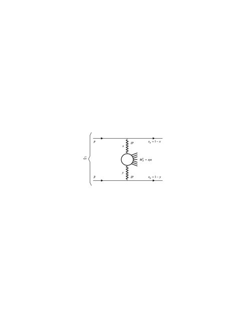
FIG. 1.: IGM picture for a double Pomeron exchange process.

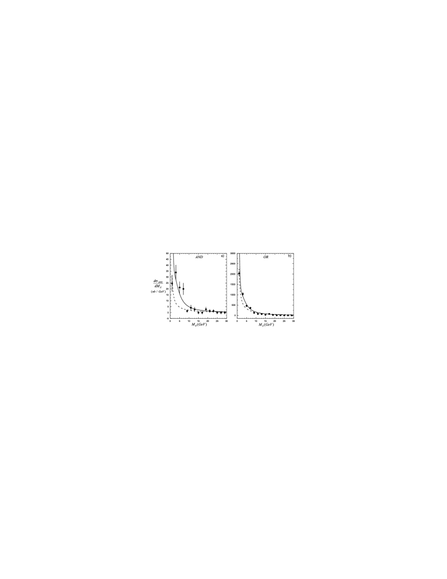
FIG. 2.: IGM DPE diffractive mass distributions: Solid and dashed lines show the numerical results with $\sigma_{I\!\!PI\!\!P}$ equal to $0.5\,mb$ and $1.0\,mb$, respectively. Our curves were normalized to the “AND” (a) and “OR” (b) data samples of [1].

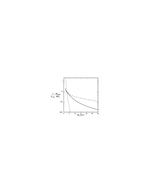
FIG. 3.: IGM DPE diffractive mass distributions, in arbitrary units, with $p_{d}=0.025$ (dash-dotted line), $0.05$ (solid line) and $0.1$ (dashed line). In all cases $\sigma_{I\!\!PI\!\!P}=0.5\,mb$.

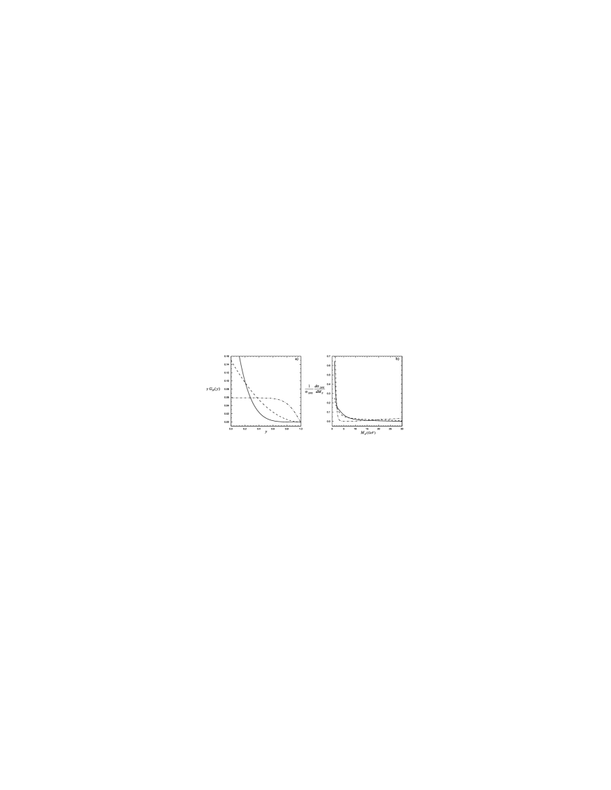
FIG. 4.: a) Diffractive gluon distributions: solid line was calculated with Eq. (15), dashed and dash-dotted lines, calculated by Eq. (14), represent the “hard” and “super-hard” Pomeron profiles, given respectively by Eq. (10) and (11); b) Diffractive mass distributions, normalized to the unity, for the same cases showed in a). In all cases $p_{d}=0.05$ and $\sigma_{I\!\!PI\!\!P}=0.5\,mb$.

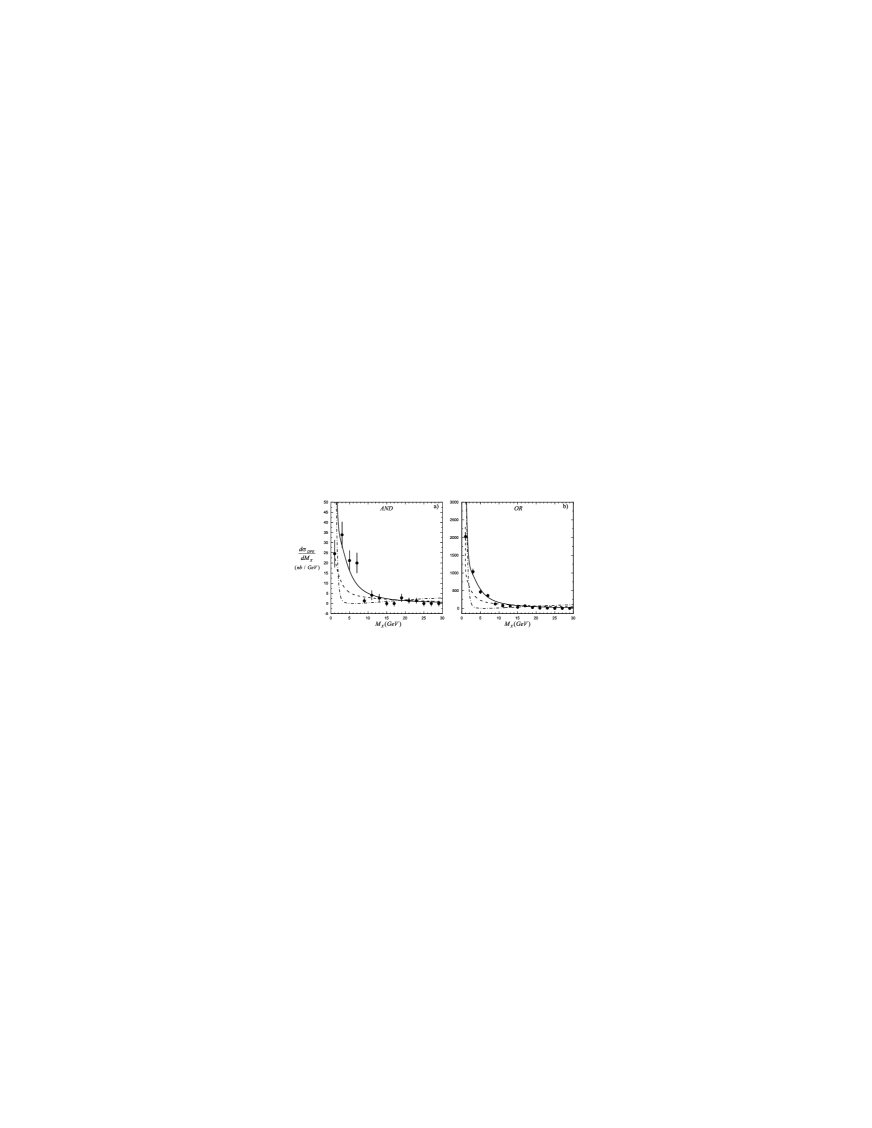
FIG. 5.: IGM DPE diffractive mass distributions: Solid, dashed and dash-dotted lines follow the same notation of Fig. 4. Our curves were obtained with $p_{d}=0.05$ and $\sigma_{I\!\!PI\!\!P}=0.5\,mb$ and normalized to the data samples of [1].

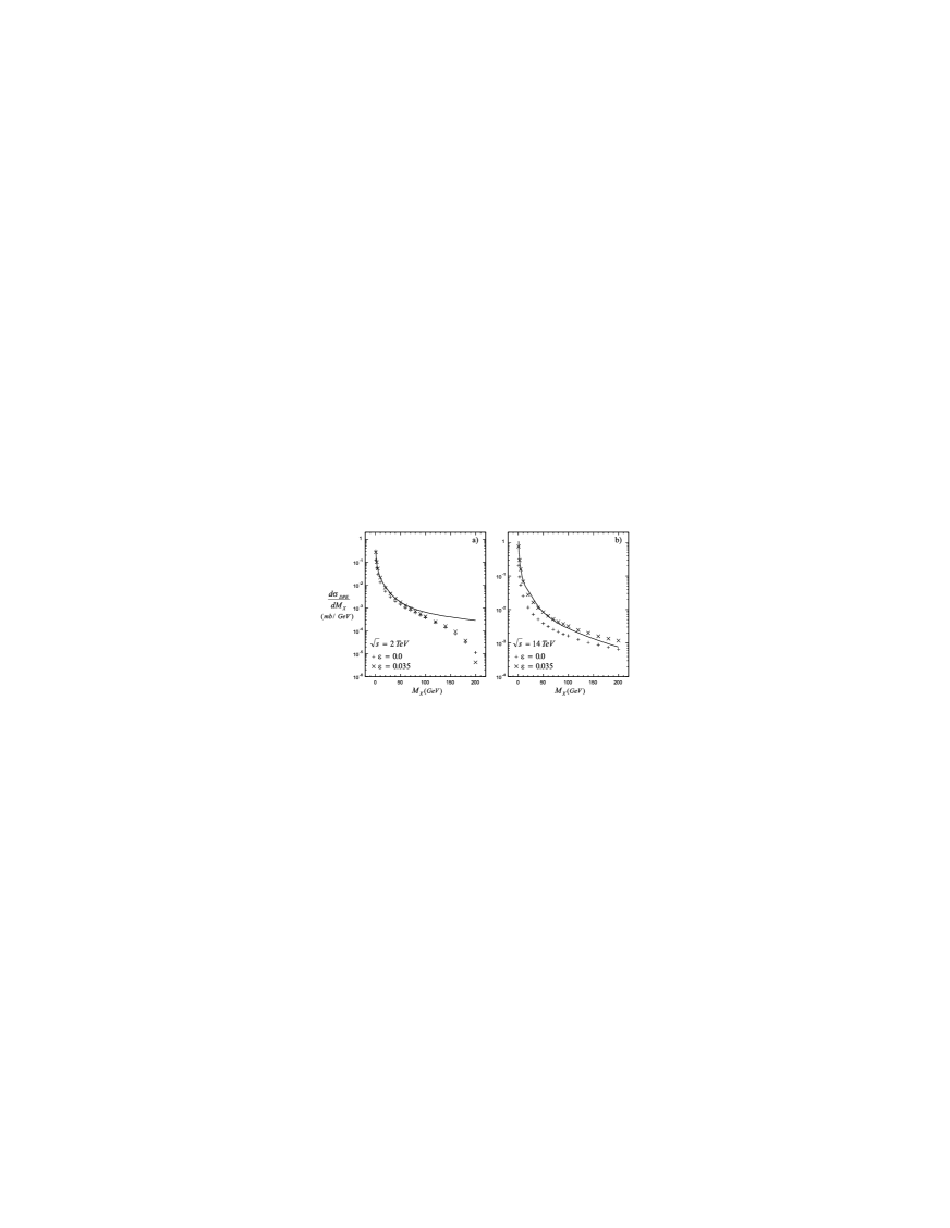
FIG. 6.: IGM predictions for $d\sigma/dM_{X}$ at Tevatron and at LHC with $\sigma_{I\!\!PI\!\!P}=1.0\,mb$. Cross($+$) and Cross($\times$) are predictions made by Brandt et al. [1] for two values of effective Pomeron intercepts $\alpha(0)=1+\varepsilon$.

FIG. 7.: Ratio double/single Pomeron exchange mass distributions as a function of $M_{X}$. In both cases we have assumed $\sigma_{I\!\!PI\!\!P}=1.0\,mb$ (for DPE processes) and $\sigma_{pI\!\!P}=1.0\,mb$ (for SPE processes).

FIG. 8.: Double and single Pomeron exchange normalized rapidity ($Y_{X}$) distributions. In both cases we have assumed $\sigma_{I\!\!PI\!\!P}=1.0\,mb$ (for DPE processes) and $\sigma_{pI\!\!P}=1.0\,mb$ (for SPE processes).

REFERENCES

• [1] A. Brandt et al., UA8 Collaboration, Eur. Phys. J. C25, (2002) 361.
• [2] J.C. Collins, L. Frankfurt and M. Strikman, Phys. Lett. B307, (1993) 161.
• [3] A. Berera and D.E. Soper. Phys. Rev. D53, (1996) 6162.
• [4] A. Berera and J.C. Collins, Nucl. Phys. B474, (1996) 183.
• [5] L. Alvero, J.C. Collins, J. Terron and J.J. Witmore, Phys. Rev. D59, (1999) 074022.
• [6] A. Berera, Phys. Rev. D62, (2000) 014015.
• [7] G.N. Fowler, F.S. Navarra, M. Plümer, A. Vourdas, R.M. Weiner and G. Wilk, Phys. Rev. C40, (1989) 1219.
• [8] K. Goulianos, Acta Phys. Polon. B33, (2002) 3467.
• [9] F.O. Durães, F.S. Navarra and G. Wilk, Phys. Rev. D55, (1997) 2708 and references therein.
• [10] F.O. Durães, F.S. Navarra and G. Wilk, Phys. Rev. D56, (1997) R2449.
• [11] F.O. Durães, F.S. Navarra and G. Wilk, Phys. Rev. D58, (1998) 094034.
• [12] F.O. Durães, F.S. Navarra and G. Wilk, Mod. Phys. Lett. A13, (1998) 2873 and Braz. J. Phys. 28, (1998) 505.
• [13] X.N. Wang, Phys. Rev. D43, (1991) 104; X.N. Wang and M. Gyulassy, Phys. Rev. D45, (1992) 844.
• [14] A. di Giacomo and H. Panagopoulos, Phys. Lett. B285, (1992) 133.
• [15] For a review of instanton calculations, see T. Schaefer and E. Shuryak, Rev. Mod. Phys. 70, (1998) 323.
• [16] E.V. Shuryak and I. Zahed, Phys. Rev. D62, (2000) 085014; E.V. Shuryak, Phys. Lett. B486, (2000) 378.
• [17] F.O. Durães, F.S. Navarra and G. Wilk, Phys. Rev. D47, (1993) 3049; Phys. Rev. D50, (1994) 6804; F.O. Durães, F.S. Navarra, C.A.A. Nunes and G. Wilk, Phys. Rev. D53, (1996) 6136.
• [18] J. Breitweg et al., ZEUS Collaboration, Eur. Phys. J. C5, (1998) 41.
• [19] C. Adloff et al., H1 Collaboration, Z. Phys. C74, (1997) 221.
• [20] M. Derrick et al., ZEUS Collaboration, Phys. Lett. B356, (1995) 129; Z. Phys. C68, (1995) 569.
• [21] T. Ahmed et al., H1 Collaboration, Nucl. Phys. B435, (1995) 3; B429, (1994) 477.
Refer to caption