Solar Neutrinos: Interpretation of Results

Abstract

Recent SNO results give strong evidence that the solar neutrinos undergo the flavor conversion. Main issue now is the identification of the mechanism of conversion. The LMA MSW solution with $\Delta m^{2}=(5-7)\cdot 10^{-5}$ eV², $\tan^{2}\theta=0.35-0.45$ looks rather plausible: it fits well the experimental data and our new theoretical prejudices. In the LMA case, KamLAND should see (0.5 - 0.7) reduced signal. VAC-QVO and LOW are accepted at about $3\sigma$-level. The SMA solution is practically excluded. No sub-leading effects produced by $U_{e3}$ and admixture of sterile neutrino have been found. The fit becomes worse with increase of $U_{e3}$ (for LMA) and the $\nu_{s}$ admixture. Still (30 - 50)% presence of the sterile neutrino is allowed. Solutions based on the neutrino spin-flip in the magnetic fields of the Sun as well as on non-standard neutrino interactions give good fit of the data. If KamLAND confirms LMA MSW, the spin-flip and non-standard interactions can be considered (and will be searched for) as sub-leading effects.

1 INTRODUCTION

The SNO results [1, 2, 3, 4] have led to breakthrough in the solar neutrino studies. Main conclusion is that solar neutrinos undergo the flavor conversion

$$\nu_{e}\rightarrow\nu_{\mu},\nu_{\tau}~{}~{}{\rm or/and}~{}~{}\bar{\nu}_{\mu},\bar{\nu}_{\tau}.$$ (1)

The key word is “appearance”: the appearance of the muon and tau neutrinos in the solar neutrino flux. Moreover, it seems, $\nu_{\mu}$ and $\nu_{\tau}$ compose larger part of the solar neutrino flux at high energies. These results further confirm earlier indications of $\nu_{\mu},\nu_{\tau}$ appearance from comparison of signals in the Homestake [5], and Kamiokande / SuperKamiokande (SK) [6] experiments, and later from comparison of fluxes determined by CC SNO results [1] and the $\nu e-$scattering events at Super-Kamiokande [6, 7].

The main issue now is to identify the mechanism of neutrino conversion.

This review is written about two months after the conference. During this time a number of new studies of the solar neutrino data have been published. Some new points have been realized but general picture and conclusions have not been changed. I will present an updated analysis, including the latest SAGE [8] and GNO [9] results.

This review is written several weeks (months?) before announcement of the KamLAND result which may put final “dot” in the long story of solar neutrino problem and make substantial part of the discussion below to be irrelevant.

2 PROFILE OF THE EFFECT

Identifying the mechanism of conversion one looks for signatures in the energy and time dependence of observables.

2.1 The energy profile

Present data allow to reconstruct the energy dependence of the effect without reference to certain mechanism of conversion [10, 11, 12]. The only assumption is that sterile neutrinos, if exist, do not participate in the solar neutrino conversion. Schematically the procedure of reconstruction can be performed in the following three steps (see, e.g., [13, 14] for earlier analysis).

1).“SNO NC/CC and SK/SNO”. Using the SK and SNO data one can get the averaged survival probability above $E>5$ MeV independently on the SSM predictions of fluxes. According to SNO and SK there is no substantial dependence of the survival probability on energy. Therefore the average probability $P_{ee}$ can be immediately obtained from the ratio of the CC and NC event rates:

$$P_{ee}=\frac{CC}{NC}=0.345^{+0.045}_{-0.040}.$$ (2)

2).“Cl - SK/SNO over SSM”. The SK and SNO data allow to evaluate original boron neutrino flux, and consequently, to calculate the contribution of this flux to the $Ar$-production rate $Q_{Ar}$ . Subtracting this contribution from the rate measured in Homestake one finds the contribution of fluxes of intermediate energies (0.8 - 1.5) MeV to $Q_{Ar}$. Then using the SSM predictions for the fluxes of $Be$, $pep$ and $CNO$-cycle neutrinos one gets the survival probability $P_{ee}(0.8-1.5{\rm MeV})$.

3).“Ga - Cl - SK/SNO over SSM”. Using $P_{ee}(0.8-1.5{\rm MeV})$ found in the previous step and SSM fluxes of $Be$ , $pep$ and $CNO$-cycle neutrinos one can estimate contributions of these fluxes to the $Ge$-production rate, $Q_{Ge}$. Subtracting this contributions as well as the contribution of boron neutrinos from $Q_{Ge}$ measured by SAGE and GNO/GALLEX one gets the contribution of $pp$-neutrinos to $Q_{Ge}$. Then using the SSM prediction for the $pp$-neutrino flux one finds $P_{ee}(0.2-0.4{\rm MeV})$.

Figure 1: The profile of the effect. Shown are the reconstructed values of the survival probability in different energy ranges. The lines correspond to the survival probability for the LMA and LOW solutions; (from [12]).

The result of such a type of analysis is shown in fig. 1 taken from [12]. The best profile (which corresponds to the central values of reconstructed $P_{ee}$) would have constant $P_{ee}$ at high energies, stronger suppression at the intermediate energies and weak suppression at low energies. The profile can not be reproduced by LMA or LOW solutions. Although these solutions are in agreement with reconstructed profile within the error bars. Notice that the errors of reconstructed values of $P_{ee}$ at different energies strongly correlate: higher value of $P_{ee}$ at the intermediate energies corresponds to lower value of $P_{ee}$ at low energies. The reconstructed profile can be reproduced precisely by the resonance spin-flavor precession.

2.2 Time variations

1). 11 years variations related to the solar activity cycle: no variations have been found in SK, SAGE and GALLEX/GNO experiments. The cause of possible changes of the Homestake rate still unclear.

2). Seasonal variations: SK data are in agreement with geometrical (eccentricity) effect. No statistically significant variations of $Ge$-production rate have been found [8, 9].

3). Monthly variations which can be related to rotation of the Sun: it is argued that gallium and Clorine results show time variations with the several weeks period [15]. The claim is based on direct analysis of time dependence of experimental signals as well as on bi-normal distribution of number of bins with a given rate in GALLEX/GNO and SAGE. It should be stressed, however, that GNO results alone do not show bi-normal distribution [9].

4). Diurnal variations: the day-night asymmetries measured by SK and SNO(CC) experiments are

$$-A^{ES}_{DN}=2.1\pm 2.0~{}^{+1.3}_{-1.2}\%,$$ (3)

$$-A^{CC}_{DN}=7.0\pm 4.9~{}^{+1.5}_{-1.4}\%.$$ (4)

The later is obtained under constraint that total flux has no D-N asymmetry [3]. Although the results are not statistically significant, they have the expected sign and values. The difference of asymmetries at SNO and SK is explained by the dumping factor for ES signal due to effect of $\nu_{\mu},\nu_{\tau}$ [16]. For LMA and LOW solutions we get

$$A_{DN}^{CC}=\left[1+\frac{r}{(1-r)P_{ee}}\right]A_{DN}^{ES},$$ (5)

where $r\equiv\sigma(\nu_{\mu}e)/\sigma(\nu_{e}e)$. The effect is significant (in spite of small $r$) since the $\nu_{\mu}/\nu_{\tau}$ flux is 2 - 4 times larger than the $\nu_{e}-$ flux. Taking $P_{ee}$ from (2) we get for LMA: $A_{DN}^{CC}=1.53A_{DN}^{ES}$, in agreement (within 1$\sigma$) with the experimental results.

3 GLOBAL FIT

Implications of new SNO results have been studied in [12, 17, 18, 19, 20, 21, 22, 23, 24]. Here I will present our updated analysis [21] which includes, in particular, new GNO results.

3.1 Input

Data. In the analysis we use (1) three rates: $Q_{Ar}$, (Homestake experiment [5]), $Q_{Ge}$, from SAGE [8], and combined $Q_{Ge}$ from GALLEX and GNO [9]; (2) the zenith-spectra measured by Super-Kamiokande [6] during 1496 days [6, 7]; (3) the day and the night energy spectra of all events measured at SNO [4]. Altogether there are 81 data points.

Neutrino Fluxes. The boron neutrino flux (the dimensionless quantity $f_{B}\equiv F_{B}/F_{B}^{SSM}$), is treated as free parameter. The SSM boron neutrino flux is $F^{SSM}_{B}=5.05\cdot 10^{6}$ cm^-2 s^-1. All other neutrino fluxes and their uncertainties are taken according to SSM BP2000 [25]. For the $hep-$neutrino flux we use fixed value $F_{hep}=9.3\times 10^{3}$ cm^-2 s^-1 [25, 26] .

In the case of two neutrinos there are three fit parameters: $\Delta m^{2}$, $\tan^{2}\theta$, $f_{B}$, and therefore 81(data points) - 3 = 78 d.o.f. .

3.2 LMA MSW

Figure 2: The global LMA MSW solution. The best fit point is marked by a star. The allowed regions are shown at 1$\sigma$, 90% C.L., 2$\sigma$, 99% C.L. and 3$\sigma$. Also shown are the lines of constant NC/CC ratio.

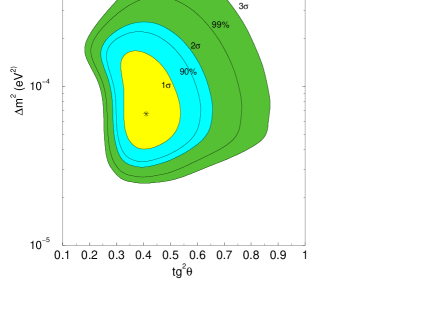
In the best fit point (see fig. 2)

$$\begin{array}[]{l}\Delta m^{2}=6.15\cdot 10^{-5}~{}{\rm eV}^{2},~{}~{}~{}\tan^{2}\theta=0.41,\\ f_{B}=1.05,\end{array}$$ (6)

we get $\chi^{2}/dof=65.2/78$. In fig. 2 we show also the lines of constant ratio NC/CC. The best fit point corresponds to ${\rm NC/CC}=3.15$. The best fit values and $3\sigma$ intervals for $Ar-$ and $Ge-$ production rates equal

$$Q_{Ar}=2.95~{}^{+0.40}_{-0.25}~{}{\rm SNU},~{}~{}Q_{Ge}=70.5~{}^{+13.5}_{-7.5}~{}{\rm SNU}.$$ (7)

The grid of predicted values of DN-asymmetry in CC is shown in fig. 3.

How large is the large mixing? The upper limit on mixing angle is controlled by the following observables:

$$\begin{array}[]{l}\frac{CC}{NC}\sim\sin^{2}\theta,~{}~{}~{}Q_{Ar}\sim f_{B}\sin^{2}\theta,\\ Q_{Ge}\sim 1-\frac{1}{2}\sin^{2}2\theta.\end{array}$$ (8)

The global fit gives

$$\tan^{2}\theta<0.84,~{}~{}99.73\%~{}~{}{\rm C.L.}.\\$$ (9)

Figure 3: Lines of constant day-night asymmetry of CC events. In the best fit point: $A_{DN}^{CC}=3.9\%$.

There is a significant spread of the bounds obtained by different groups: 0.55 [3], 0.64 [12], 0.89 [17] $(99.73\%~{}~{}{\rm C.L.})$. In any case, we have a strong evidence that solar neutrino mixing significantly deviates from maximal value. The parameter [27]

$$\epsilon\equiv 1-2\sin^{2}\theta,$$ (10)

which characterizes the deviation of mixing from the maximal one, equals [21]

$$\epsilon>0.08,~{}~{}~{}(3\sigma).$$ (11)

That is, at $3\sigma$: $\epsilon>\sin^{2}\theta_{c}$, where $\theta_{c}$ is the Cabibbo angle. This result has important implications for the neutrinoless double beta decay searches, determination of the absolute mass scale of neutrinos, theory of neutrino masses. Maximal mixing is accepted at $4\sigma$ level in the range $\Delta m^{2}=(7-10)\cdot 10^{-5}$ eV². For maximal mixing we get: NC/CC $<2~{}~{}(-2.2\sigma)$, $Q_{Ar}\sim 3.2~{}{\rm SNU}~{}~{}(+2.8\sigma)$, $Q_{Ge}\sim 64~{}{\rm SNU}~{}~{}(-1.8\sigma)$, $f_{B}=0.85$.

How high is the high $\Delta m^{2}$? The upper bound on $\Delta m^{2}$ has important implications for measurements of $\Delta m^{2}$ itself, future LBL experiments, determination of the CP-violating phase, etc.. From the global fit we find

$$\Delta m^{2}\leq 3.6\times 10^{-4}~{}{\rm eV}^{2},~{}~{}99.73\%~{}{\rm C.L.}$$ (12)

which is stronger than the CHOOZ bound [28].

3.3 Physics of LMA

Physical processes depend on neutrino energy and values of oscillation parameters (see e.g. [29, 30] for recent discussion). According to the LMA MSW solution (with the parameters (6)) neutrinos undergo the adiabatic conversion inside the Sun.

1). For high energy neutrinos ($E>5$ MeV) the conversion has a character of non-oscillatory adiabatic transformation $\nu_{e}\rightarrow\nu_{2}$, with final survival probability $P_{ee}\approx\sin^{2}\theta$. In matter of the Earth $\nu_{2}$ oscillates leading to $\nu_{e}$ regeneration effect which increases with energy and can reach few per cents (see, e.g., [30]).

2). In the intermediate energy range ($0.8-2$ MeV) there is an interplay of the conversion and oscillations. The later are averaged out.

3). At low energies ($E<0.5$ MeV) the effect is reduced to vacuum oscillations with small matter corrections: $P^{(2)}_{ee}\rightarrow(1-0.5\sin^{2}2\theta_{12})$.

3.4 Pro and Contra

1). LMA does not reproduce perfectly the energy profile of the effect. LMA predicts larger $Q_{Ar}$ than the Homestake rate. It is not excluded, however, that Homestake has some unknown systematic error.

2). No one signature of the LMA has been observed with high statistical significance: There is no turn up of the spectrum at low energies, although, the present sensitivity is not enough to observe the effect. There is no significant regeneration effect. At the same time both SK and SNO data give some indications of the day-night asymmetries which have correct sign and correct relative values.

3). The oscillation solution of the atmospheric neutrino problem makes rather plausible interpretation of the solar neutrino results in terms of vacuum mixing and masses. Also large/maximal mixing observed in atmospheric neutrinos give the precedent for large mixing in conversion of solar neutrinos.

4). In the case of LMA MSW the hierarchy of solar and atmospheric $\Delta m^{2}$ is the weakest which is natural in presence of large mixing.

3.5 Predictions for KamLAND

Figure 4: Lines of constant suppression of the rate at KamLAND, $R_{Kam}$, (figures at the curves).

The discussion of pro and contra LMA will be irrelevant after the KamLAND results [31]. The effect of oscillation disappearance can be characterized by the ratio, $R_{Kam}$, of the total number of events with visible energy $T>2.6$ MeV with and without oscillations. In fig. 4 the contours of constant suppression factor $R_{Kam}$ are shown in the $\Delta m^{2}-\tan^{2}\theta$ plot. Details of calculations can be found in [21]. In the best fit point we find $R_{Kam}=0.65$, the $1\sigma$ region is $R_{Kam}=0.4-0.7$, and in $3\sigma$ region: $R_{Kam}=0.25-0.73$. The value $R_{Kam}>0.75$ will be problematic for the LMA. The distortion of the visible energy spectrum depends on $\Delta m^{2}$ strongly. The most profound effect of oscillations is suppression of the rate at high energies. For instance, for $E\approx 5$ MeV and b.f. value of $\Delta m^{2}$ the suppression is stronger than 1/2.

4 ALTERNATIVES

Viable alternatives to LMA MSW can be divided in to three categories, depending on mechanism of conversion: (1) LOW MSW and VO-QVO related to transformations induced by neutrino masses and vacuum mixing. (2) Solutions based on neutrino spin-flip in the magnetic fields of the Sun. Here there are two possibilities: the flip in the convective zone, and in the radiative zone of the Sun. Furthermore, the effect of flip can have resonance or non-resonance character. (3) Conversion induced by non-standard neutrino interactions. For all these solutions (but VO), the matter effects play crucial role.

4.1 Mass and mixing solutions

1). VAC-QVO next best?. In the best fit point

$$\begin{array}[]{l}\Delta m^{2}=4.5\cdot 10^{-10}~{}{\rm eV}^{2},~{}~{}~{}\tan^{2}\theta=2.1,\\ f_{B}=0.75,\end{array}$$ (13)

we get $\chi^{2}(VAC)-\chi^{2}(LMA)=9.7$. The solution is accepted at $3\sigma$ level. It appears in the dark side of the parameter space so that some matter effect is present. Features of this solution “discovered” in 1998 are: absence of any day-night asymmetry, low ($-1.6\sigma$) Boron neutrino flux, high ($+2.7\sigma$) Ar-production rate: $Q_{Ar}=3.2$ SNU, low ($-2.6\sigma$) ratio: NC/CC$=1.86$.

2) LOW starts to disappear? In the best fit point

$$\begin{array}[]{l}\Delta m^{2}=0.93\cdot 10^{-7}~{}{\rm eV}^{2},~{}~{}~{}\tan^{2}\theta=0.64,\\ f_{B}=0.91,\end{array}$$ (14)

we get $\chi^{2}(LOW)-\chi^{2}(LMA)=12.4$ which is slightly beyond the $3\sigma$ range. In other analyses, LOW does appear at $3\sigma$ level. Inclusion of the SK data which contain information about zenith angle distribution (zenith spectra) worsens the fit (see comments in [22]).

The LOW solution gives rather poor fit of total rates. In the best fit point we get large ($+2.1\sigma$) $Ar-$production rate: $Q_{Ar}=3.2$ SNU and $1.2\sigma$ lower $Ge-$production rate: $Q_{Ge}=66.5$ SNU. The ratio NC/CC$=2.35$ is in agreement with observations. For the day-night asymmetry of the CC-events we predict $A_{DN}^{CC}=-3.5\%$ and for ES events: $A_{DN}^{CC}=-2.7\%$.

3). Any chance for SMA? In the best fit point

$$\begin{array}[]{l}\Delta m^{2}=5.0\cdot 10^{-6}~{}{\rm eV}^{2},~{}~{}~{}\tan^{2}\theta=5.0\cdot 10^{-4},\\ f_{B}=0.58,\end{array}$$ (15)

we get $\chi^{2}(SMA)-\chi^{2}(LMA)=34.5$. So, SMA is accepted at $5.5\sigma$ only. Moreover, the solution requires about $3\sigma$ lower boron neutrino flux than in the SSM. It predicts positive Day-Night asymmetry: $A_{DN}^{CC}=0.93\%$. Very bad fit is due to latest SNO measurements of the day and night spectra. We find $NC/CC\approx 1/P_{ee}=1.37$ which is substantially smaller than the observed quantity (2). Contribution of the $NC$ events is suppressed which leads to distortion of the energy spectrum of all events in comparison with observations. At the same time, SMA provides rather good description of the SK data: the rate and spectra. (We find that $\chi^{2}$ increases weakly with $\tan^{2}\theta$ up to $\tan^{2}\theta=1.5\cdot 10^{-3}$, where $\chi^{2}\sim 105$.)

The solution is practically excluded unless some systematic error will be found in the SNO or/and SK results.

4.2 Pull-off diagrams.

Figure 5: Pull-off diagrams for the LMA, VAC and LOW solutions. The pull-offs are expressed in the units of 1 standard deviation, $1\sigma$.

The pull-off diagrams (fig. 5, [32, 21], see [23] for extensive discussion of the pull method) show deviations, $D_{K}$, of the predicted value of observable $K$ in the best fit point from the central experimental value expressed in the $1\sigma$ unit, $\sigma_{K}$,:

$$D_{K}\equiv\frac{K_{bf}-K_{exp}}{\sigma_{K}},~{}~{}~{}~{}$$ (16)

$K\equiv Q_{Ar},~{}Q_{Ge},$  NC/CC,  $R_{\nu e},~{}A_{DN}^{SK},A_{DN}^{CC}$. We take the experimental errors only: $\sigma_{K}=\sigma_{K}^{exp}$.

According to the pull-off diagram the LMA solution reproduces observables at $\sim 1\sigma$ or better. LOW and VAC give worse fit to the data.

5 LEADING AND SUB-LEADING

Identification of the solution means, first of all, the identification of the leading effect in solar neutrinos. LMA MSW is rather plausible candidate. Apart from the leading mechanism a number of sub-leading effects can be present.

According to available data, $U_{e3}$, mixing of sterile neutrinos, and neutrino decay can only produce sub-leading effects.

Status of the neutrino spin-flip in the magnetic field of the Sun as well as non-standard neutrino interactions is not yet clear. These mechanisms can be leading or produce sub-leading effects, if e.g., LMA MSW turns out to be the solution. Also a possibility of the hybrid solutions is not excluded when two (or more) different effects give comparable contributions to the conversion: for instance, MSW conversion and the spin-flip [33, 34].

5.1 Solar neutrinos and $U_{e3}$

Let us consider the neutrino mass spectrum which explains the solar and atmospheric neutrino data. The mass eigenstates $\nu_{1}$ and $\nu_{2}$ are split by the solar $\Delta m^{2}_{12}$, whereas the third mass eigenstate, $\nu_{3}$, is separated by mass difference determined by the atmospheric $\Delta m^{2}_{13}$. Matter effect influences mixing (flavor content) of the third mass eigenstate very weakly. The effect of third neutrino is reduced then to averaged vacuum oscillations, and the probability equals

$$P_{ee}=\cos^{4}\theta_{13}P_{ee}^{(2)}+\sin^{4}\theta_{13}.$$ (17)

Here $\sin\theta_{13}\equiv U_{e3}$, $P_{ee}^{(2)}$ is the two neutrino oscillation probability characterized by $\tan^{2}\theta_{12}$, $\Delta m_{12}^{2}$ and the effective matter potential reduced by factor $\cos^{2}\theta_{13}$ (see e.g. [35, 36] for related studies).

Figure 6: Global LMA solution for $\sin^{2}\theta_{13}=0.04$. The best fit point is marked by a star.

Mainly, the effect of $\theta_{13}$ consists of overall suppression of the survival probability. The suppression factor can be as small as 0.90 - 0.92. Results of the global analysis in the three neutrino context are shown in fig. 6. We use the three neutrino survival probability (17) for fixed value $\sin^{2}\theta_{13}=0.04$ (near the upper bound from the CHOOZ experiment [28]), so that number of degrees of freedom is the same as in the previous analysis. In the best fit point:

$$\Delta m^{2}_{12}=6.7\cdot 10^{-5}{\rm eV}^{2},~{}~{}\tan^{2}\theta=0.41,$$ (18)

and $f_{B}=1.09$. The best fit value of $\Delta m^{2}_{12}$ is slightly higher than that in the two neutrino case. The changes are rather small, however, as a tendency, with increase of $\theta_{13}$ the fit becomes worse in comparison with $2\nu-$ case: for $\sin^{2}\theta_{13}=0.04$ we get $\Delta\chi^{2}=1.0$. The detailed study of the conversion in $3\nu-$ context is given in [36].

For LOW solution increase of $\theta_{13}$ leads to improvement of the fit, so that this solution appears (for $\sin^{2}\theta_{13}=0.4$) at 3$\sigma$ level with respect to best fit point (18).

5.2 Sterile neutrinos

Oscillations to pure sterile state: $\nu_{e}\rightarrow\nu_{s}$ are excluded at $5\sigma$ level [2]. So, the sterile neutrinos, if exist, may produce a sub-leading effect, or be a part of “hybrid” solution. The analysis has been performed in the context of single $\Delta m^{2}$ conversion $\nu_{e}\rightarrow\nu_{x}$, where

$$\nu_{x}=\cos\eta~{}\nu_{a}+\sin\eta~{}\nu_{s}.$$ (19)

In this case $\nu_{e}$ undergo transitions to $\nu_{e},\nu_{\mu,\tau},\nu_{s}$ inside the Sun with the following probabilities:

$$\nu_{e}\rightarrow\left\{\begin{array}[]{ll}\nu_{e},&P_{ee}\\ \nu_{a},&(1-P_{ee})\cos^{2}\eta\\ \nu_{s},&(1-P_{ee})\sin^{2}\eta\\ \end{array}.\right.$$ (20)

The matter potential is modified: $V=\sqrt{2}G_{F}(n_{e}-0.5\sin^{2}\eta n_{n})$, where $n_{e}$ and $n_{n}$ are the densities of the electrons and neutrons correspondingly. According to (20) fluxes of neutrinos detected by the charged current (CC), neutral current reaction (NC) and the neutrino-electron scattering (ES) equal respectively:

$$\begin{array}[]{l}\Phi_{CC}=f_{B}P_{ee}\\ \Phi_{NC}=f_{B}[1-(1-P_{ee})\sin^{2}\eta]\\ \Phi_{ES}=f_{B}[P_{ee}-r(1-P_{ee})\cos^{2}\eta]\\ \end{array}.$$ (21)

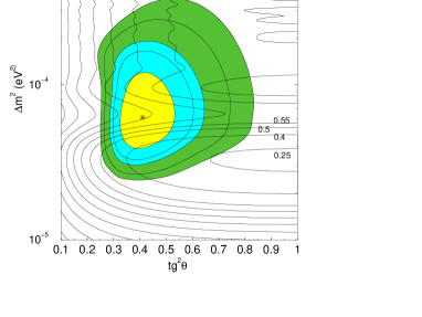
The fluxes (21) depend on two combinations of three parameters: $f_{B}P_{ee}$ and $f_{B}(1-P_{ee})\cos^{2}\eta$. So, degeneracy of parameters takes place and increase of $\eta$ can be compensated by changes of $f_{B}$ and $P_{ee}$ [12]. The degeneracy is broken by energy dependence of the probability and by the Earth regeneration effect. Since both effects are small (according to the data), only weak bound on admixture of sterile neutrino follows from the present data (see fig. 7 from [37]). In the analysis [37] for each pair of values of ($\cos^{2}\eta$, $f_{B}$), $\chi^{2}$ is minimized with respect to $\Delta m^{2},\tan^{2}\theta$, thus function $\chi^{2}(\cos^{2}\eta,f_{B})$ has been found which was used to construct the confidence level contours in fig. 7. The absolute minimum of $\chi^{2}$ corresponds to no sterile neutrino: $\sin^{2}\eta=0,~{}~{}~{}f_{B}=1.07$, and the upper bound on $\eta$ is rather weak

$$\sin^{2}\eta<0.35~{}~{}(0.70),~{}~{}~{}~{}1\sigma~{}~{}(3\sigma).$$ (22)

Stronger bound can be obtained from combined analysis of the solar neutrino data and the KamLAND results.

Figure 7: Bounds on sterile neutrino admixture and the original boron neutrino flux, (from [37]).

5.3 Spin-flavor precession

Resonance spin-flavor precession [38] opens unique possibility to reconcile strong suppression of solar neutrino flux at intermediate energies and absence of distortion at high energies. For appropriate choice of the magnetic field distribution the mechanism allows to reproduce the profile of fig. 1. Analysis of the data gives values of $\Delta m^{2}$ and magnetic field in the peak [39, 40, 41, 42] :

$$\begin{array}[]{l}\Delta m^{2}=(0.8-1.5)\cdot 10^{-8}{\rm eV}^{2},\\ B=80-100{\rm kG}\end{array}$$ (23)

for the neutrino magnetic moment $\mu_{\nu}=10^{-11}\mu_{B}$. Solutions with larger values of $B$ also exist.

Non-resonance spin-flavor precession leads to profile similar to that of LMA MSW [43]. The required values of parameters are as in  (23).

No oscillation effect is expected in the KamLAND experiment if one of the spin-flip solutions is true. Furthermore, solutions based on the neutrino spin-flip do not lead to the Earth regeneration effects, in particular, to the Day-Night asymmetry.

On the other hand, long period variations of signals are generic consequences of the neutrino spin-flip in the convective zone of the Sun. Indeed, the surface magnetic field shows 11 years variations. There is no model which has constant large scale field in the convective zone and variations of the surface field [44]. Due to convective mixing large scale field in the convective zone should be seen at the surface [44].

Another variability is expected due to existence of the equatorial gap in the toroidal magnetic field and inclination of the Earth orbit with respect to solar equatorial plane. This leads to the semiannual variations of the electron neutrino flux [45].

Neither 11 years nor semiannual variations of signals have been observed. That was the motivation to revisit a possibility of the neutrino spin-flip in the radiative zone [44, 41]. It was assumed that strong relic field exists in the radiative zone. The field is frozen and therefore constant. The field has a toroidal configuration with maximal strength $B=(0.4-0.6)$ MG at $R\sim 0.15R_{\odot}$. The survival probability is given by

$$P_{ee}=0.5[1-(1-2P_{c})\cos 2\theta_{0}],$$ (24)

where $P_{c}$ is the level crossing probability and $\theta_{0}$ is the mixing angle in the production point. To describe experimental data one needs to have $P_{ee}\sim 0.3$, that is, the flip should be non-adiabatic. Notice that in the non-adiabatic case it is rather non-trivial to have weak energy distortion of the spectrum.

The profile of the effect is similar to the profile for LMA, and the data are well described for $\Delta m^{2}=(1.5-5.0)10^{-6}$ eV² [44].

5.4 Non-standard neutrino interactions

Both mixing and level splitting required for neutrino conversion can be induced by the neutrino interaction with matter [46]. The corresponding terms in the effective Hamiltonian (mixing, $\bar{H}$, level splitting, $H$) can be parameterized in the following way:

$$\begin{array}[]{l}H=\sqrt{2}G_{F}[n_{e}(r)-\epsilon^{\prime}n_{f}(r)]\\ \bar{H}=\sqrt{2}G_{F}[\epsilon n_{f}(r)],\end{array}$$ (25)

where $f=u,d$ (-quarks). There is no dependence of the probability on neutrino energy: $P_{ee}=const$. The dependence of the effect on energy appears due to difference of the production regions for $pp-$, $Be-$ and $B-$neutrinos. The average densities in the production region satisfy inequalities $n(pp)<n(Be)<n(B)$. The larger the density the stronger conversion. In such a way the LMA type profile of the effect is well reproduced. Global fit of the data leads to the best values of parameters [40]:

$$\epsilon,~{}~{}\epsilon^{\prime}=\left\{\begin{array}[]{lll}3\cdot 10^{-3},&0.60,&f=u\\ 1.5\cdot 10^{-3},&0.43,&f=d\end{array}\right..$$ (26)

The problem here is that very large value of the diagonal coupling $\epsilon^{\prime}$ is required which is difficult to reconcile with the experimental bounds in the context of known models for $\epsilon,\epsilon^{\prime}$. The solution predicts earth regeneration effect, however no oscillation signal in KamLAND is expected.

6 CONCLUSION

LMA MSW with parameters $\Delta m^{2}\sim(5-7)\cdot 10^{-5}$ eV² and $\tan^{2}\theta=0.35-0.45$ is rather plausible solution. It fits well experimental data and our new theoretical prejudices. In this sense, the present status of LMA is similar to the status of SMA 5 years ago… So, some surprises are not excluded.

What could be alternative? The QVO-VO and LOW solutions are accepted at about $3\sigma$ level. SMA is excluded at more than $5\sigma$ level. Solutions based on neutrino spin-flip in the solar magnetic field or non-standard neutrino interactions (flavor changing and flavor diagonal) are rather appealing from the point of view of the data fit, but they have their own disadvantages. Hopefully, the situation will be clarified by KamLAND, further operation of SNO and, later, BOREXINO [47].

In the context of LMA MSW, (as well as LOW) recent SNO results lead to important bounds on neutrino parameters: Now we have strong evidence that “solar” mixing is non-maximal, and moreover, deviation from maximal mixing is rather large: $\tan^{2}\theta<0.8$ ($3\sigma$). Possible effect of $U_{e3}$ is small being disfavored by data. The admixture of sterile component is further restricted: $\sin^{2}\eta<0.35-0.50$.

The LMA MSW solution will be tested soon by the KamLAND experiment: in the best fit point one expects the suppression factor for integral signal $\sim 0.6-0.7$ (0.3 - 0.75 at $3\sigma$) and the spectrum distortion with substantial suppression in the high energy part.

Soon, solar neutrino studies can be transformed to new stage when emphasis will be on determination of the original neutrino fluxes and searches for the sub-dominant effects produced by $U_{e3}$, admixture of sterile neutrino both in one and more than one $\Delta m^{2}$ context, magnetic moment of neutrino, non-standard interactions, etc..