Recoil momentum spectrum in directional dark matter detectors

Abstract

Directional dark matter detectors will be able to record the recoil momentum spectrum of nuclei hit by dark matter WIMPs. We show that the recoil momentum spectrum is the Radon transform of the WIMP velocity distribution. This allows us to obtain analytic expressions for the recoil spectra of a variety of velocity distributions. We comment on the possibility of inverting the recoil momentum spectrum and obtaining the three-dimensional WIMP velocity distribution from data.

I Introduction

The identification of dark matter is one of the major open questions in physics, astrophysics, and cosmology. Recent cosmological observations together with constraints from primordial nucleosynthesis point to the presence of non-baryonic dark matter in the universe. The nature of this non-baryonic dark matter is still unknown.

One of the preferred candidates for non-baryonic dark matter is a weakly interacting massive particle (WIMP). Substantial efforts have been dedicated to WIMP searches in the last decades review . A particularly active area dm2002 are WIMP direct searches, in which low-background devices are used to search for the nuclear recoil caused by the elastic scattering of galactic WIMPs with nuclei in the detector goodman-witten . In these searches, characteristic signatures of a WIMP signal are useful in discriminating a WIMP signal against background.

A WIMP signature which was pointed out very early freese is an annual modulation of the direct detection rate caused by the periodic variation of the Earth velocity with respect to the WIMP “sea” while the Earth goes around the Sun. The typical amplitude of this modulation is 5%. A modulation with these characteristics was observed by the DAMA collaboration dama , but in light of recent results cdms ; edelweiss , its interpretation as a WIMP signal is currently in question. Different, and possibly clearer, WIMP signatures would be beneficial.

A stronger modulation, with an amplitude that may reach 100%, was pointed out by Spergel in 1988 s88 . Spergel noticed that because of the Earth motion around the Sun, the most probable direction of the nuclear recoils changes with time, describing a full circle in a year. In particular this produces a strong forward-backward asymmetry in the angular distribution of nuclear recoils.

Unfortunately it has been very hard to build WIMP detectors sensitive to the direction of the nuclear recoils. A promising development is the DRIFT detector DRIFT . The DRIFT detector consists of a negative ion time projection chamber, the gas in the chamber serving both as WIMP target and as ionization medium for observing the nuclear recoil tracks. The direction of the nuclear recoil is obtained from the geometry and timing of the image of the recoil track on the chamber end-plates. A 1 m³ prototype has been successfully tested, and a 10 m³ detector is under consideration.

In addition to merely using directionality for background discrimination, what can be learned about WIMP properties from the directionality of WIMP detectors? It is obvious that different WIMP velocity distributions give rise to different recoil distributions in both energy and recoil direction. Copi, Heo, and Krauss chk , and then Copi and Krauss copi-krauss , have examined the possibility of distinguishing various WIMP velocity distributions using a likelihood analysis of the resulting recoil spectra, which they generated through a Monte Carlo program. They have concluded that a discrimination among common velocity distributions is possible with a reasonable number of detected events.

Here we want to gain insight into the properties of the nuclear recoil spectra in energy and direction. For this purpose, we develop a simple formalism that relates the WIMP velocity distribution to the distribution of recoil momenta. We find that the recoil momentum spectrum is the Radon transform of the velocity distribution (see Eq. (17) below). We apply this analytical tool to a series of velocity distributions, and discover for example how the recoil momentum spectrum of a stream of WIMPs differs from that of a Maxwellian velocity distribution. With our gained insight, we suggest that if a WIMP signal is observed in directional detectors in the future, it may be possible to invert the measured recoil momentum spectrum and reconstruct the WIMP velocity distribution from data.

In Section II we describe the general kinematics of elastic WIMP-nucleus scattering, and in Section III we obtain our main formula for the nuclear recoil momentum spectrum. Sections IV and V contain general considerations and examples of Radon transforms of velocity distributions. Finally, Section VI discusses the possibility of inverting the recoil momentum spectrum to recover the WIMP velocity distribution. The Appendices contain useful mathematical formulas for the computation and inversion of 3-dimensional Radon transforms.

II WIMP-nucleus elastic scattering

Consider the elastic collision of a WIMP of mass $m$ with a nucleus of mass $M$ in the detector (see Fig. 1). Let the arrival velocity of the WIMP at the detector be ${\bf v}$, and neglect the initial velocity of the nucleus. After the collision, the WIMP is deflected by an angle $\theta^{\prime}$ to a velocity ${\bf v}^{\prime}$, and the nucleus recoils with momentum ${\bf q}$ and energy $E=q^{2}/2M$. Let $\theta$ denote the angle between the initial WIMP velocity ${\bf v}$ and the direction of the nuclear recoil ${\bf q}$. Energy and momentum conservation impose the following relations:

$$\frac{1}{2}mv^{2}=\frac{1}{2}mv^{\prime 2}+\frac{q^{2}}{2M},$$ (1)

$$mv^{\prime}\cos\theta^{\prime}=mv-q\cos\theta,\phantom{\frac{1}{2}}$$ (2)

$$mv^{\prime}\sin\theta^{\prime}=q\sin\theta.\phantom{\frac{1}{2}}$$ (3)

Eliminating $\theta^{\prime}$ by summing the squares of Eqs. (2) and (3),

$$m^{2}v^{\prime 2}=(mv-q\cos\theta)^{2}+(q\sin\theta)^{2}=m^{2}v^{2}-2mvq\cos\theta+q^{2},$$ (4)

and using this expression to eliminate $v^{\prime}$ from Eq. (1), gives

$$q=2\mu v\cos\theta,$$ (5)

where

$$\mu=\frac{mM}{m+M}$$ (6)

is the reduced WIMP-nucleus mass. We deduce that the magnitude $q$ of the recoil momentum, and the recoil energy $E$, vary in the range

$$0\leq q\leq q_{\rm max}\equiv 2\mu v,\qquad 0\leq E\leq E_{\rm max}\equiv\frac{2\mu^{2}v^{2}}{M}.$$ (7)

Eq. (5) will be exploited in the following Section to express the recoil momentum distribution in a simple mathematical form. For this purpose, we also need the expression for the WIMP-nucleus scattering cross section. We write the differential WIMP-nucleus scattering cross section as

$$\frac{d\sigma}{dq^{2}}=\frac{\sigma_{0}}{q_{\rm max}^{2}}S(q),$$ (8)

where $\sigma_{0}$ is the total scattering cross section of the WIMP with a (fictitious) point-like nucleus, and $S(q)=|F(q)|^{2}$ is a nuclear form factor normalized so that $S(0)=1$. (Both $S(q)$ and $F(q)$ are confusingly called form factors.) Eq. (8) is valid for both spin-dependent and spin-independent WIMP-nucleus interactions, although $\sigma_{0}$ and $F(q)$ have different expressions in the two cases. For example, for spin-independent interactions with a nucleus with $Z$ protons and $A-Z$ neutrons,

$$\sigma_{0}=\frac{\mu^{2}}{\pi}\left[ZG^{p}_{s}+(A-Z)G^{n}_{s}\right]^{2},$$ (9)

where $G^{p}_{s}$ and $G^{n}_{s}$ are the scalar four-fermion couplings of the WIMP with pointlike protons and neutrons, respectively (see Ref. lesarcs ). If the nucleus can be approximated by a sphere of uniform density, its form factor is

$$F(q)=\frac{9[\sin(qR)-qR\cos(qR)]^{2}}{(qR)^{6}},$$ (10)

where

$$R\simeq[0.91A^{1/3}+0.3]\times 10^{-13}{\rm cm}$$ (11)

is (an approximation to) the nuclear radius. More realistic expressions for spin-independent form factors, and formulas for spin-dependent cross sections, can be found, e.g., in Refs. lesarcs ; lewinsmith ; jkg ; tovey .

III Recoil momentum spectrum

Eqs. (5) and (8) can be combined to give the differential recoil spectrum in both energy and direction, i.e. the recoil momentum spectrum. We define it as the double differential event rate, in events per unit time per unit detector mass, differentiated with respect to the nuclear recoil energy $E$ and the nuclear recoil direction $\widehat{\bf q}$,

$$\frac{dR}{dEd\Omega_{q}},$$ (12)

where $d\Omega_{q}$ denotes an infinitesimal solid angle around the direction $\widehat{\bf q}$.

The double differential rate follows from the double differential cross section

$$\frac{d\sigma}{dq^{2}d\Omega_{q}}$$ (13)

first through the change of differentials $dq^{2}=2MdE$, and then through multiplication by the number $N$ of nuclei in the detector, division by the detector mass $MN$, and multiplication by the flux of WIMPs with velocities ${\bf v}$ in the velocity space element $d^{3}v$,

$$nvf({\bf v})\,d^{3}v.$$ (14)

Here $n=\rho/m$ is the WIMP number density, $\rho$ is the WIMP mass density, and $f({\bf v})$ is the WIMP velocity distribution in the frame of the detector, normalized to unit integral.

The double differential cross section is obtained as follows. Azimuthal symmetry of the scattering around the WIMP arrival direction gives $d\Omega_{q}=2\pi\,d\!\cos\theta$. The relation between $\cos\theta$ and $q$ in Eq. (5), $\cos\theta=q/2\mu v$, can be imposed through a Dirac $\delta$ function, $\delta(\cos\theta-q/2\mu v)$. Thus

$$\frac{d\sigma}{dq^{2}d\Omega_{q}}=\frac{d\sigma}{dq^{2}}\,\,\frac{1}{2\pi}\,\,\delta\!\left(\cos\theta-\frac{q}{2\mu v}\right)=\frac{\sigma_{0}S(q)}{8\pi\mu^{2}v}\,\,\delta\!\left(v\cos\theta-\frac{q}{2\mu}\right).$$ (15)

This is correctly normalized as can be seen by integration of the expression in the middle over $d\Omega_{q}$.

Summarizing, the double differential event rate per unit time per unit detector mass is

$$\frac{dR}{dEd\Omega_{q}}=2M\,\frac{N}{MN}\int\frac{d\sigma}{dq^{2}d\Omega_{q}}\,\,n\,v\,f({\bf v})\,d^{3}v=\frac{n\sigma_{0}S(q)}{4\pi\mu^{2}}\int\delta\!\left(v\cos\theta-\frac{q}{2\mu}\right)\,f({\bf v})\,d^{3}v.$$ (16)

We write it as

$$\frac{dR}{dEd\Omega_{q}}=\frac{n\sigma_{0}S(q)}{4\pi\mu^{2}}\,\,\widehat{f}(v_{q},\widehat{\bf q}).$$ (17)

Here

$$v_{q}=\frac{q}{2\mu}=\sqrt{\frac{ME}{2\mu^{2}}}$$ (18)

is the minimum velocity a WIMP must have to impart a recoil momentum $q$ to the nucleus, or equivalently to deposit an energy $E=q^{2}/2M$, as can be seen from Eq. (7). Moreover,

$$\widehat{f}(w,\widehat{\bf w})=\int\delta({\bf v}\cdot\widehat{\bf w}-w)\,f({\bf v})\,d^{3}v,$$ (19)

is the 3-dimensional Radon transform of the velocity distribution function $f({\bf v})$. We note in passing that $\widehat{f}$ has units of inverse speed.

Eq. (17) is the main result of this paper. It states that, apart from a normalizing factor, the recoil momentum spectrum is the Radon transform of the WIMP velocity distribution. The Radon transform is a linear integral transform (see Refs. d83 ; rk96 ), which was introduced in two dimensions by Radon in 1917 r17 . The Radon transform has been widely studied for its use in solving differential equations, and especially in two-dimensions, for its medical applications in computer tomography. Geometrically, $\widehat{f}(w,\widehat{\bf w})$ is the integral of the function $f({\bf v})$ on a plane orthogonal to the direction $\widehat{\bf w}$ at a distance $w$ from the origin. For reference, some mathematical properties of the Radon transform are given in the Appendices.

As a check of our formalism, we show that integrating our basic equation (17) over recoil directions reproduces the usual expression for the recoil energy spectrum $dR/dE$. Applying Eq. (49) in Appendix A to our expression for the differential rate, we find

$$\frac{dR}{dE}=\frac{n\sigma_{0}S(q)}{2\mu^{2}}\,\,\int_{v>q/2\mu}\frac{f({\bf v})}{v}\,\,d^{3}v.$$ (20)

This is the usual expression of the recoil energy spectrum (cfr. Eq. (8.3) in Ref. jkg ).

IV Computing the recoil momentum spectrum

We have cast the nuclear recoil momentum spectrum in terms of a Radon transform. Now we can take advantage of the properties of Radon transforms, some of which are listed in the Appendices, to compute recoil momentum spectra analytically. In this Section we give some general considerations, and in the next Section we give explicit examples of analytic recoil momentum spectra.

IV.1 Isotropic distributions

When the WIMP velocity distribution is isotropic, $f({\bf v})=f(v)$, the recoil spectrum is also isotropic, $\widehat{f}(w,{\bf w})=\widehat{f}(w)$. From the definition of Radon transform, Eq. (19),

$$\widehat{f}(w)=2\pi\int_{w}^{\infty}f(v)vdv.$$ (21)

We would have obtained the same result starting from Eq. (49).

IV.2 Moving observer

WIMP velocity distributions are often given in the galactic rest frame, while we are interested in the recoil momentum spectrum in the laboratory frame of the detector. The change of velocity frame can be performed either on the velocity distribution before computing the Radon transform or on the Radon transform computed in the galactic rest frame. The latter is often easier to compute, and the change of reference frame can be done simply as follows.

The WIMP velocities ${\bf v}_{\rm lab}$ and ${\bf v}_{\rm gal}$ in the laboratory and galactic rest frames, respectively, are related by

$${\bf v}_{\rm lab}={\bf v}_{\rm gal}-{\bf V}_{\rm lab},$$ (22)

where ${\bf V}_{\rm lab}$ is the velocity of the laboratory with respect to the galactic rest frame. This velocity transformation is a translation in velocity space, and we can use Eq. (46) in Appendix A to relate the Radon transforms in the galactic and laboratory frames,

$$\widehat{f}_{\rm lab}(w,\widehat{\bf w})=\widehat{f}_{\rm gal}(w+{\bf V}_{\rm lab}\cdot\widehat{\bf w},\widehat{\bf w}).$$ (23)

Thus the recoil momentum spectrum in the laboratory frame is given directly in terms of the Radon transform $\widehat{f}_{\rm gal}(w,\widehat{\bf w})$ of the WIMP velocity distribution in the galactic rest frame by

$$\frac{dR}{dEd\Omega_{q}}=\frac{n\sigma_{0}S(q)}{4\pi\mu^{2}}\,\,\,\widehat{f}_{\rm gal}\!\left(v_{q}+{\bf V}_{\rm lab}\cdot\widehat{\bf q},\,\widehat{\bf q}\right),$$ (24)

with $v_{q}=q/2\mu$ as before.

IV.3 Rotated observer

If we rotate the coordinate system, we see from Eq. (45) in Appendix A that the recoil momentum spectrum is simply rotated, with the magnitude of the recoil momentum remaining the same, as expected.

V Examples of recoil momentum spectra

We give some examples of recoil momentum spectra corresponding to common velocity distributions. We obtain the recoil spectra for streams of particles and for isotropic and anisotropic Gaussian distributions with and without bulk velocities.

V.1 A WIMP stream or flow

The simplest case is that of a particle stream in which all WIMPs in the stream move with the same velocity ${\bf V}$. In this case,

$$f_{\rm stream}({\bf v})=\delta({\bf v}-{\bf V}),$$ (25)

and

$$\widehat{f}_{\rm stream}(w,\widehat{\bf w})=\delta({\bf V}\cdot\widehat{\bf w}-w).$$ (26)

The recoil spectrum of a stream with velocity ${\bf V}$ is concentrated on a sphere of radius $V/2$, centered in ${\bf V}/2$ and passing through the origin. The stream velocity ${\bf V}$ is a diameter of the sphere.

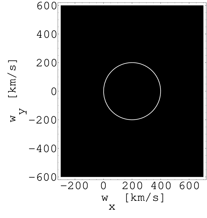
Figure 2: Probability density distribution of the nuclear recoil momentum in the recoil plane $(w_{x},w_{y})$, assuming a stream of WIMPs with velocity $(v_{x},v_{y},v_{z})=(400\,{\rm km/s},0,0)$. The full $(w_{x},w_{y},w_{z})$ distribution can be obtained by revolution around the $w_{x}$ axis. The recoil momenta describe a sphere in recoil space.

Fig. 2 shows the $(w_{x},w_{y})$ section of the recoil momentum spectrum of a stream of WIMPs arriving from the left with velocity $V_{x}=400$ km/s. The full distribution is obtained through a rotation around the $w_{x}$ axis. The pattern of recoil momenta forms a sphere.

V.2 Maxwellian distribution

A Maxwellian distribution with velocity dispersion $\sigma_{v}$,

$$f_{\rm M}(v)=\frac{1}{(2\pi\sigma_{v}^{2})^{3/2}}\exp\left[{-\frac{v^{2}}{2\sigma_{v}^{2}}}\right],$$ (27)

is a particular case of isotropic distribution, and we can use Eq. (21) above to compute its Radon transform. We find

$$\widehat{f}_{\rm M}(w)=\frac{1}{(2\pi\sigma_{v}^{2})^{1/2}}\exp\left[{-\frac{w^{2}}{2\sigma_{v}^{2}}}\right].$$ (28)

If the detector has velocity ${\bf V}_{\rm lab}$, we can use Eq. (23) to find the Radon transform in the laboratory frame,

$$\widehat{f}_{\rm M,lab}(w,\widehat{\bf w})=\frac{1}{(2\pi\sigma_{v}^{2})^{1/2}}\exp\left[{-\frac{\left[w+\widehat{\bf w}\cdot{\bf V}_{\rm lab}\right]^{2}}{2\sigma_{v}^{2}}}\right].$$ (29)

Notice that $\widehat{\bf w}\cdot{\bf V}_{\rm lab}$ is the projection of the velocity of the observer in the direction of the nuclear recoil. This expression coincides with, but is simpler than, the analogous expression obtained by elementary methods in Ref. s88 ($\cos\gamma$ in Ref. s88 is $\cos\gamma=-\widehat{\bf w}\cdot\widehat{\bf V}_{\rm lab}$).

The recoil momentum distribution for a Maxwellian distribution is shown in Fig. 3, assuming a velocity dispersion of 300 km/s and an observer moving at 220 km/s in direction $-x$. The distribution is symmetric around the observer velocity. The figure shows the section in the $(w_{x},w_{y})$ plane only. The full distribution can be obtained by symmetry.

Eq. (29) illustrates the reason for writing $\widehat{f}(w,\widehat{\bf w})$ instead of $\widehat{f}({\bf w})$ (see Section A.1 for more details). The function $\widehat{f}_{\rm M,lab}(0,\widehat{\bf w})$ assumes different values for different directions $\widehat{\bf w}$; the function $\widehat{f}({\bf w})$ would therefore be multivalued at the origin.

V.3 Truncated Maxwellian distribution

We may truncate a Maxwellian distribution at the escape speed $v_{\rm esc}$,

$$f_{\rm TM}(v)=\begin{cases}\displaystyle\frac{1}{N_{\rm esc}(2\pi\sigma_{v}^{2})^{3/2}}\exp\left[{-\frac{v^{2}}{2\sigma_{v}^{2}}}\right],&v<v_{\rm esc}\cr 0,&{\rm otherwise}\end{cases},$$ (30)

with

$$N_{\rm esc}={\rm erf}\!\left(\frac{v_{\rm esc}}{\sqrt{2}\sigma_{v}}\right)-\sqrt{\frac{2}{\pi}}\frac{v_{\rm esc}}{\sigma_{v}}\exp\left[{-\frac{v_{\rm esc}^{2}}{2\sigma_{v}^{2}}}\right].$$ (31)

Then we have

$$\widehat{f}_{\rm TM}(w)=\frac{1}{N_{\rm esc}(2\pi\sigma_{v}^{2})^{1/2}}\left\{\exp\left[{-\frac{w^{2}}{2\sigma_{v}^{2}}}\right]-\exp\left[{-\frac{v_{\rm esc}^{2}}{2\sigma_{v}^{2}}}\right]\right\}.$$ (32)

V.4 Non-isotropic Gaussian distribution

The recoil-momentum spectrum corresponding to an anisotropic Gaussian distribution can also be obtained analytically. An anisotropic Gaussian distribution with variance matrix $\bm{\sigma}^{2}$ and mean velocity ${\bf V}$ is given by

$$f_{\rm gauss}({\bf v})=\frac{1}{(8\pi^{3}\det\bm{\sigma}^{2})^{1/2}}\exp\left[{-\frac{({\bf v}-{\bf V})^{T}\bm{\sigma}^{-2}\,({\bf v}-{\bf V})}{2}}\right].$$ (33)

We are using matrix notation, ${\bf v}^{T}$ being the transpose of ${\bf v}$, etc. Using the Fourier slice theorem, actually Eq. (51), we find the Radon transform of the anisotropic Gaussian to be

$$\widehat{f}_{\rm gauss}(w,\widehat{\bf w})=\frac{1}{(2\pi\,\widehat{\bf w}^{T}\bm{\sigma}^{2}\,\widehat{\bf w})^{1/2}}\exp\left[{-\frac{\left[w-\widehat{\bf w}\cdot{\bf V}\right]^{2}}{2\widehat{\bf w}^{T}\!\bm{\sigma}^{2}\,\widehat{\bf w}}}\right].$$ (34)

This is another example of a function which assumes different values at $w=0$ according to the direction $\widehat{\bf w}$.

VI Reconstructing the velocity distribution

The recoil spectrum of a stream and a Maxwellian velocity distribution are very different: a sphere the first, a smooth distribution the second. This suggests that it may be possible to distinguish different kinds of WIMP velocity distributions just by examining the pattern of recoil momenta. Subtle differences among velocity distributions may be revealed by a maximum likelihood analysis of the corresponding recoil spectra chk ; copi-krauss .

More ambitiously, we may think of recovering the WIMP velocity distribution by inverting the measured recoil momentum spectrum. Indeed, if we know the nuclear form factor of the detector nuclei, then for any fixed WIMP mass we can estimate the Radon transform of the WIMP velocity distribution from the measured recoil momentum spectrum, modulo a normalization constant $K$. Eq. (17) can in fact be written as

$$\widehat{f}(v_{q},\widehat{\bf q})=K\,\frac{4\pi\mu^{2}}{S(q)}\,\frac{dR}{dEd\Omega_{q}},$$ (35)

enabling us to obtain a measurement of the Radon transform $\widehat{f}(v_{q},\widehat{\bf q})$ of the WIMP velocity distribution from the measured recoil spectrum $dR/dEd\Omega_{q}$. We may be able to invert this Radon transform and obtain the WIMP velocity distribution $f({\bf v})$, again modulo a normalization constant. Finally, we may be able to fix the normalization constant either by normalizing $f({\bf v})$ to unit integral or better by examining the detector efficiency as a function of WIMP velocity.

There are several analytic formulas for the inversion of three-dimensional Radon transforms. Some of these formulas are collected in Appendix B for convenience. Most of the analytical inversion formulas can be converted into numerical algorithms . However, any inversion algorithm we were able to find in the literature is suited only to a large amount of data in recoil momentum space, since they all assume that it would be possible to define a discretized version of $\widehat{f}(w,\widehat{\bf w})$. This is not the case for directional dark matter searches, where the total number of events is not under the control of the experimentalist and is expected to be rather small.

New inversion algorithms suited to small numbers of events are therefore needed if one wants to reconstruct the WIMP velocity distribution using data from directional detectors. As a first attempt in this direction, we have devised the following simple algorithm. Divide the WIMP velocity space into small cells $S_{m}$, $m=1,\dots,M$, and assume that the WIMP velocity distribution $f({\bf v})$ is constant over each of these small cells, with value $f_{m}$ in cell $S_{m}$. To each recorded event $j$ with measured recoil momentum ${\bf q}_{j}$, $j=1,\ldots,N$, associate the plane $P_{j}$ in WIMP velocity space defined by the equation

$$P_{j}:\quad 2\mu{\bf v}\cdot\widehat{\bf q}_{j}=q_{j}.$$ (36)

$P_{j}$ is the plane orthogonal to the recoil direction $\widehat{\bf q}_{j}$ and at a distance $w_{j}=q_{j}/2\mu$ from the origin. Velocity vectors on this plane are all the WIMP velocities that can produce the observed nuclear recoil. Let

$$a_{jm}={\rm area}(S_{m}\cap P_{j}),$$ (37)

the area of the intersection of the plane $P_{j}$ with the cell $S_{m}$ (see Appendix C for an explicit expression). For each event $j$, assign weight $a_{jm}$ to the $m$-th cell. Sum the weights over the events, $A_{m}=\sum_{j=1}^{N}a_{jm}$, essentially counting how many planes cross any given cell. Take the discrete Laplacian of the sum of the weights, and keep only those cells whose values exceed a predetermined threshold. The resulting distribution of cell values is our estimate of the WIMP velocity distribution.

To test the capabilities of our algorithm, we simulated the recoil spectrum due to two streams of WIMPs arriving at the detector from opposite directions, with velocities $(V_{1x},V_{1y},V_{1z})=(0,0,0.5)$ and $(V_{2x},V_{2y},V_{2z})=(0,0,-0.2)$ (in arbitrary units). We generated 100 events, and applied the previous algorithm with $64^{3}$ cells in velocity space and a threshold of $0.1$. We found that only two cells in velocity space are above threshold, and they correspond exactly to the location of the simulated streams. Fig. 4 plots the $(v_{x},v_{z})$ section of the reconstructed velocity distribution. It is impressive that we were able to recover this velocity distribution with only 100 events.

We leave further studies of our simple algorithm, and the development of other algorithms, to future work.

VII Conclusions

Directional detectors for WIMP dark matter searches will be able to measure not only the energy but also the direction of the nuclear recoils caused by the elastic scattering of galactic WIMPs with nuclei in the detector. This directional capability will help in separating a WIMP signal from background, and will also provide a measurement of the recoil momentum spectrum as compared to just the recoil energy spectrum.

To gain insight into the properties of recoil momentum spectra, we have devised a simple formalism for the analytic computation of recoil momentum spectra from WIMP velocity distributions. Mathematically, the recoil momentum spectrum is the 3-dimensional Radon transform of the velocity distribution.

Well-established mathematical properties of the Radon transform allow the computation of analytical expressions for recoil spectra associated to several common WIMP velocity distributions. As examples we presented recoil spectra for a WIMP stream, a Maxwellian, a truncated Maxwellian, and a non-isotropic Gaussian. We found in particular that a stream of WIMPs produces a characteristic spherical pattern of nuclear recoils. A Maxwellian distribution gives instead a smooth recoil pattern. Other velocity distributions lead to more complicated spectra.

The analytic expressions we found for the nuclear recoil spectra will facilitate the discrimination of different velocity distributions through likelihood analysis. In addition, it may be possible to invert the measured momentum spectrum to reconstruct the local WIMP velocity distribution from data. For this purpose, we have presented an algorithm to recover the velocity distribution from a small number of recorded events. We have successfully recovered a simulated velocity distribution with just 100 generated events.

We expect that the tools we have presented will be useful for the design and analysis of directional WIMP detectors.

Appendix A Some mathematics of the Radon transform

In this appendix we collect some useful mathematical properties of the 3-dimensional Radon transform. We denote the 3-dimensional Radon transform of a function $f({\bf v})$ by $\widehat{f}(w,\widehat{\bf w})$. It is defined by

$$\widehat{f}(w,\widehat{\bf w})=\int\delta(w-\widehat{\bf w}\cdot{\bf v})f({\bf v})d^{3}v.$$ (38)

It is easy to see that the Radon transform is linear,

$$\widehat{f_{1}+f_{2}}=\widehat{f_{1}}+\widehat{f_{2}}.$$ (39)

A.1 A remark on notation

One may be tempted to write $\widehat{f}({\bf w})$ for $\widehat{f}(w,\widehat{\bf w})$, after all ${\bf w}=w\widehat{\bf w}$. This notation may however be ambiguous and should be used with care. Indeed, one must keep in mind that the Radon transform as defined in Eq. (38) is a function of the magnitude $w$ and the direction $\widehat{\bf w}$ separately. In other words, one may have $\widehat{f}(0,\widehat{\bf w})\neq\widehat{f}(0,\widehat{\bf w}^{\prime})$ for $\widehat{\bf w}\neq\widehat{\bf w}^{\prime}$. Namely, $\widehat{f}(0,\widehat{\bf w})$ may assume different values for different directions. This will not be reflected in the notation $\widehat{f}({\bf w})$. The latter would read $\widehat{f}(0)$ at the origin, independently of the direction $\widehat{\bf w}$. In other words, $\widehat{f}({\bf w})$ would be a multiple-valued function at the origin. Mathematically, the distinction between $\widehat{f}(w,\widehat{\bf w})$ and $\widehat{f}({\bf w})$ is important, and is expressed by saying that $\widehat{f}(w,\widehat{\bf w})$ is defined on $\mathbb{R}\times S^{2}$ while $\widehat{f}({\bf w})$ is defined on $\mathbb{R}^{3}$. For our application, however, the distinction is of little concern, since the problematic origin $w=0$ corresponds to the region of vanishingly small recoil momenta, which is experimentally inaccessible. We have nevertheless used the mathematically correct notation throughout for clarity.

A.2 Change of coordinates

Under linear transformations of the coordinate axes, ${\bf v}$ transforms as

$${\bf v}\to{\bf v}^{\prime}={\rm A}{\bf v}+{\bf b},$$ (40)

where ${\rm A}$ is a $3\times 3$ non-singular matrix and ${\bf b}$ is a constant vector. A velocity distribution function $f({\bf v})$ transforms so as to keep the number of particles in a volume $d^{3}v$ invariant:

$$f^{\prime}({\bf v}^{\prime})d^{3}v^{\prime}=f({\bf v})d^{3}v.$$ (41)

Hence,

$$f^{\prime}({\bf v}^{\prime})=\frac{1}{|\!\det{\rm A}|}\,f\!\left({\rm A}^{-1}({\bf v}^{\prime}-{\bf b})\right),$$ (42)

where $\det{\rm A}$ is the determinant of ${\rm A}$ and ${\rm A}^{-1}$ is the inverse of ${\rm A}$. To find the relation between the Radon transforms of $f({\bf v})$ and $f^{\prime}({\bf v}^{\prime})$, we change integration variable from ${\bf v}^{\prime}$ to ${\bf v}$ in the definition, Eq. (38),

$$\widehat{f^{\prime}}(w^{\prime},\widehat{\bf w}^{\prime}) = \int\delta(w^{\prime}-\widehat{\bf w}^{\prime}\cdot{\bf v}^{\prime})\,f^{\prime}({\bf v}^{\prime})\,d^{3}v^{\prime}=\int\delta(w^{\prime}-\widehat{\bf w}^{\prime}\cdot{\rm A}{\bf v}-\widehat{\bf w}^{\prime}\cdot{\bf b})\,f({\bf v})\,d^{3}v$$ (43)

$$= \int\delta(w^{\prime}-\widehat{\bf w}^{\prime}\cdot{\bf b}-{\rm A}^{\!T}\widehat{\bf w}^{\prime}\cdot{\bf v})\,f({\bf v})\,d^{3}v=\widehat{f}(w^{\prime}-\widehat{\bf w}^{\prime}\cdot{\bf b},{\rm A}^{\!T}\widehat{\bf w}^{\prime}),$$

where ${\rm A}^{\!T}$ is the transpose of ${\rm A}$. Thus

$$\widehat{f^{\prime}}(w^{\prime},\widehat{\bf w}^{\prime})=\widehat{f}(w^{\prime}-\widehat{\bf w}^{\prime}\cdot{\bf b},\,{\rm A}^{\!T}\widehat{\bf w}^{\prime}).$$ (44)

In particular, under a pure rotation ${\rm R}$,

$$\widehat{f^{\prime}}(w^{\prime},\widehat{\bf w}^{\prime})=\widehat{f}(w^{\prime},\,{\rm R}^{-1}\widehat{\bf w}^{\prime}),$$ (45)

and under a pure translation ${\bf b}$,

$$\widehat{f^{\prime}}(w^{\prime},\widehat{\bf w}^{\prime})=\widehat{f}(w^{\prime}-\widehat{\bf w}^{\prime}\cdot\widehat{\bf b},\,{\bf w}^{\prime}).$$ (46)

A.3 Transformation of derivatives

The following relations hold for derivatives of the Radon transform (here ${\bf v}=(v_{1},v_{2},v_{3})$ and ${\bf w}=(w_{1},w_{2},w_{3})$)

$$\widehat{\frac{\partial f}{\partial v_{k}}}=\frac{w_{k}}{w}\frac{\partial\widehat{f}}{\partial w},$$ (47)

$$\frac{\partial\widehat{f}}{\partial w_{k}}=-\frac{1}{w}\frac{\partial}{\partial w}\widehat{v_{k}f}.$$ (48)

A.4 Integration over angles

We find the following expression for the integral of the Radon transform $\widehat{f}(w,\widehat{\bf w})$ over the directions $\widehat{\bf w}$:

$$\int\widehat{f}(w,\widehat{\bf w})d\Omega_{w} = \int\int\delta({\bf v}\cdot\widehat{\bf w}-w)\,f({\bf v})\,d^{3}v\,d\Omega_{w}=\int\left[\int\delta({\bf v}\cdot\widehat{\bf w}-w)\,d\Omega_{w}\right]\,f({\bf v})\,d^{3}v$$ (49)

$$= \int\left[2\pi\int_{-1}^{1}\delta(v\cos\gamma-w)\,d\!\cos\gamma\right]\,f({\bf v})\,d^{3}v=\int\frac{2\pi}{v}\,\theta(v-|w|)\,\,f({\bf v})\,d^{3}v$$

$$= 2\pi\int_{v>|w|}\frac{f({\bf v})}{v}\,\,d^{3}v.$$

A.5 Fourier slice theorem

There is a connection between the Radon transform and the Fourier transform. Taking the Fourier transform of the definition, Eq. (38), with respect to $w$ at fixed $\widehat{\bf w}$ gives

$$\int_{-\infty}^{+\infty}d\lambda e^{i\lambda t}\widehat{f}(\lambda,\widehat{\bf w})=\int f({\bf v})e^{it\widehat{\bf w}\cdot{\bf v}}d^{3}v.$$ (50)

This equation goes under the name of Fourier slice theorem. The right hand side is just the Fourier transform of $f({\bf v})$ evaluated at $t\widehat{\bf w}$, while the left hand side is the Fourier transform of $\widehat{f}(w,\widehat{\bf w})$ at fixed $\widehat{\bf w}$.

Inverting the Fourier transform in the left hand side of the Fourier slice theorem, we have

$$\widehat{f}(w,\widehat{\bf w})=\frac{1}{2\pi}\int_{-\infty}^{\infty}dte^{-iwt}\int f({\bf v})e^{it\widehat{\bf w}\cdot{\bf v}}d^{3}v.$$ (51)

This alternative expression of the Radon transform actually serves as its definition when functions are replaced by distributions (in the mathematical sense, see Ref. rk96 ).

A.6 Expansion into spherical harmonics

Let us expand $f({\bf v})$ and its Radon transform $\widehat{f}(w,\widehat{\bf w})$ into spherical harmonics $Y_{lm}(\widehat{\bf v})$ and $Y_{lm}(\widehat{\bf w})$, respectively. We have

$$f({\bf v})=\sum_{lm}f_{lm}(v)Y_{lm}(\widehat{\bf v}),$$ (52)

and

$$\widehat{f}(w,\widehat{\bf w})=\sum_{lm}\widehat{f}_{lm}(w)Y_{lm}(\widehat{\bf w}).$$ (53)

The coefficients of the spherical harmonic expansions are related by

$$\widehat{f}_{lm}(w)=2\pi\int_{w}^{\infty}P_{l}\!\left(\frac{w}{v}\right)f_{lm}(v)vdv.$$ (54)

where $P_{l}(x)$ is a Legendre polynomial of order $l$. These expressions are useful when the velocity distributions are not isotropic.

Eq. (54) can be proven using the decomposition of the $\delta$-function in Legendre polynomials

$$\delta(\widehat{\bf v}\cdot\widehat{\bf w}-t)=\theta(1-t)\sum_{l}\frac{2l+1}{2}P_{l}(t)\,P_{l}(\widehat{\bf v}\cdot\widehat{\bf w}),$$ (55)

the addition theorem for spherical harmonics

$$P_{l}(\widehat{\bf v}\cdot\widehat{\bf w})=\frac{4\pi}{2l+1}\sum_{m=-l}^{l}Y^{*}_{lm}(\widehat{\bf v})Y_{lm}(\widehat{\bf w}),$$ (56)

and the orthogonality of the spherical harmonics

$$\int Y^{*}_{l^{\prime}m^{\prime}}(\widehat{\bf v})Y_{lm}(\widehat{\bf v})d\Omega_{v}=\delta_{l^{\prime}l}\delta_{m^{\prime}m},$$ (57)

which lead to the relation

$$\int\delta(\widehat{\bf v}\cdot\widehat{\bf w}-t)Y_{lm}(\widehat{\bf v})d\Omega_{v}=2\pi\theta(1-t)P_{l}(t)Y_{lm}(\widehat{\bf w}).$$ (58)

Appendix B Inversion formulas for the Radon transform

B.1 Inversion using the Laplacian

An inversion formula for the Radon transform is

$$f({\bf v})=-\frac{1}{8\pi^{2}}\frac{\partial^{2}}{\partial{\bf v}^{2}}\int\widehat{f}({\bf v}\cdot\widehat{\bf w},\widehat{\bf w})d\Omega_{w},$$ (59)

where $\partial^{2}/\partial{\bf v}^{2}$ is the Laplacian in ${\bf v}$. It can also be written in terms of $\widehat{f}^{\prime\prime}(w,\widehat{\bf w})=\partial^{2}\widehat{f}(w,\widehat{\bf w})/\partial w^{2}$ as

$$f({\bf v})=-\frac{1}{8\pi^{2}}\int\widehat{f}^{\prime\prime}({\bf v}\cdot\widehat{\bf w},\widehat{\bf w})d\Omega_{w},$$ (60)

The inversion formula (59) can be proven by inverting the Fourier transform of $f({\bf v})$ in the Fourier slice theorem, Eq. (50), then integrating separately in $t$ and $\widehat{\bf w}$, and finally using the relation

$$\int_{0}^{\infty}t^{2}e^{itx}dt=-\pi\delta^{(2)}(x),$$ (61)

where $\delta^{(2)}(x)$ is the second derivative of the Dirac $\delta$-function.

B.2 Inversion through spherical harmonics

Another inversion method is through an expansion in spherical harmonics. Referring to Eqs. (52) and (53), one can prove the following inversion formula

$$f_{lm}(v)=-\frac{1}{2\pi v}\int_{0}^{v}P_{l}\!\left(\frac{w}{v}\right)\widehat{f}_{lm}^{\prime\prime}(w)dw,$$ (62)

where $P_{l}(x)$ is a Legendre polynomial and $\widehat{f}_{lm}^{\prime\prime}(w)=d^{2}\widehat{f}_{lm}/dw^{2}$, the second derivative of $\widehat{f}(w)$ with respect to the modulus of $w$.

Eq. (62) is proven along the same lines as Eq. (54), starting from Eq. (60) written as

$$f({\bf v})=-\frac{1}{8\pi^{2}}\int\delta(w-{\bf v}\cdot\widehat{\bf w})\widehat{f}^{\prime\prime}(w,\widehat{\bf w})dwd\Omega_{w}.$$ (63)

B.3 Inversion through Fourier transforms

The Fourier slice theorem, Eq. (50), can be made into an algorithm for the numerical evaluation of the inverse Radon transform. Typically one would use fast Fourier transforms.

B.4 Inversion through the adjoint operator

Eq. (59) can also be made into an algorithm. For each given ${\bf v}$, the integration in $d\Omega_{w}$ amounts to an integration over the sphere of diameter ${\bf v}$ and passing through the origin (a “stream sphere”), with integration measure $d\cos(\theta/2)d\phi$ in spherical coordinates centered at the center of the sphere and north pole in ${\bf v}$. The final Laplacian can be computed numerically as the difference between the central value and the average value of its six nearest neighbors.

B.5 Algebraic inversion via discretization

An algebraic inversion method is the following (rk96, , p. 96). Suppose that the values $\widehat{f}_{j}$, $j=1,\dots,N$, corresponding to the points ${\bf w}_{j}$ are known. In medical applications, the points ${\bf w}_{j}$ form a grid or other structure in space, and the $\widehat{f}_{j}$’s are the measured signal intensities. In our case, the number of detected events may be quite small, in which case we may let ${\bf w}_{j}$ be the actual measurement of a nuclear recoil momentum, with $j$ varying over the number of events, and $\widehat{f}_{j}=1/\varepsilon_{j}$, where $\varepsilon_{j}$ is the efficiency for detecting event $j$.

By definition of Radon transform we have

$$\int_{P_{j}}f({\bf v})d^{3}v=\widehat{f}_{j},$$ (64)

where the integral is taken over the plane in ${\bf v}$-space defined by the equation

$$P_{j}:\quad{\bf v}\cdot\widehat{\bf w}=w.$$ (65)

$P_{j}$ is the plane orthogonal to the recoil direction $\widehat{\bf w}$ and at a distance $w$ from the origin. Now suppose that $f({\bf v})$ has compact support, meaning that it vanishes for $|{\bf v}|>$ something. This is a technical simplification that is valid in practice since real velocity distributions are always truncated at some large velocity (e.g. at the escape speed from the galaxy). Divide the ${\bf v}$-space into small cells $S_{m}$, $m=1,\dots,M$, and assume that $f({\bf v})$ is constant over each of these small cells, with value $f_{m}$ in cell $S_{m}$. This is the discretizing approximation. Let

$$a_{jm}={\rm area}(S_{m}\cap P_{j}),$$ (66)

be the area of the intersection of the plane $P_{j}$ with the cell $S_{m}$ (see Appendix C for an explicit expression). A discretized version of Eq. (64) is then

$$\sum_{m}a_{jm}f_{m}=\widehat{f}_{j}.$$ (67)

In matrix form

$$Af=\widehat{f},$$ (68)

where $A=(a_{jm})$ is an $N\times M$ matrix, $f=(f_{1},\dots,f_{M})^{T}$ and $\widehat{f}=(\widehat{f}_{1},\dots,\widehat{f}_{N})^{T}$. This is a system of linear equations for $f$ that can be solved by inverting $A$. Since few $a_{jm}$ differ from zero, $A$ is a sparse matrix, and it is convenient to solve this system iteratively. Fix $\omega$, $0<\omega<2$. Let the initial guess be $f^{(0)}$ and the $k$-th update be $f^{(k)}$. From $f^{(k)}$ compute the following vectors successively

$$f^{(k)}_{0} = f^{(k)},$$ (69)

$$f^{(k)}_{j} = f^{(k)}_{j-1}+\frac{\omega}{a_{j}^{2}}\left(\widehat{f}_{j}-a_{j}^{T}f^{(k)}_{j-1}\right)a_{j},\quad j=1,\dots,N.$$ (70)

Here $a_{j}^{2}=\sum_{m}a_{jm}^{2}$ and $a_{j}=(a_{j1},\dots,a_{jM})$. Finally let the next update be $f^{(k+1)}=f^{(k)}_{N}$. Ref. rk96 attributes this method to Kaczmarz.

Appendix C Area of the intersection between a plane and a cell

For future reference, we give here the expression for the area of the intersection of a plane with a rectangular cell.

Assume the $(x,y,z)$ space is divided into rectangular cells of sides $h_{x}$, $h_{y}$, and $h_{z}$ along $x$, $y$, and $z$, respectively. Let the $(i,j,k)$-th cell $S_{ijk}$ be centered in $(x_{0}+ih_{x},y_{0}+jh_{y},z_{0}+kh_{z})$,

$$S_{ijk}:\quad\left\{\begin{array}[]{l}\left(i-\frac{1}{2}\right)h_{x}+x_{0}<x<\left(i+\frac{1}{2}\right)h_{x}+x_{0},\vspace{5pt}\\ \left(j-\frac{1}{2}\right)h_{y}+y_{0}<y<\left(j+\frac{1}{2}\right)h_{y}+y_{0},\vspace{5pt}\\ \left(k-\frac{1}{2}\right)h_{z}+z_{0}<z<\left(k+\frac{1}{2}\right)h_{z}+z_{0}.\end{array}\right.$$ (71)

Let $P$ be the plane defined by

$$P:\quad\omega_{x}x+\omega_{y}y+\omega_{z}z=p.$$ (72)

Then the area of the intersection of the plane $P$ with the $(i,j,k)$-th cell $S_{ijk}$ is

$${\rm area}(S_{ijk}\cap P)\,=\,h_{x}h_{y}h_{z}\times\left\{\begin{array}[]{ll}\displaystyle 0,&\quad\hbox{if $P\sqrt{K_{1}^{2}+K_{2}^{2}+K_{3}^{2}}>\sqrt{3}/2$,}\vspace{5pt}\\ \displaystyle\frac{1}{K_{3}},&\quad\hbox{if $P\leq|K|$ and $K\geq 0$,}\vspace{5pt}\\ \displaystyle\frac{1}{K_{3}}-\frac{P^{2}+K^{2}}{K_{1}K_{2}K_{3}},&\quad\hbox{if $P\leq|K|$ and $K<0$,}\vspace{5pt}\\ \displaystyle\frac{1}{K_{3}}-\frac{(K-P)^{2}}{2K_{1}K_{2}K_{3}},&\quad\hbox{if $P>|K|$,}\end{array}\right.$$ (73)

where

$$P = \bigl{|}p-\omega_{x}(x_{0}+ih_{x})-\omega_{y}(y_{0}+jh_{y})-\omega_{z}(z_{0}+kh_{z})\bigr{|},$$ (74)

$$K = \frac{1}{2}\left(K_{3}-K_{2}-K_{1}\right),$$ (75)

and $K_{1}$, $K_{2}$, and $K_{3}$ are the quantities $|h_{x}\omega_{x}|$, $|h_{y}\omega_{y}|$, and $|h_{z}\omega_{z}|$ sorted in order of increasing magnitude, $K_{1}\leq K_{2}\leq K_{3}$. The last case in Eq. (73) becomes

$$\frac{K_{2}+K_{3}-2P}{2K_{2}K_{3}}$$ (76)

in the limit of small $K_{1}$.

Figure 1: Kinematics of elastic WIMP-nucleus scattering.

Figure 3: Probability density distribution of the nuclear recoil momentum in the recoil plane $(w_{x},w_{y})$, assuming a Maxwellian velocity distribution of WIMPs with velocity dispersion 300 km/s, and a detector moving with velocity $(V_{x},V_{y},V_{z})=(-220\,{\rm km/s},0,0)$. Lighter areas have higher probability. The full $(w_{x},w_{y},w_{z})$ distribution can be obtained by revolution around the $w_{x}$ axis.

Figure 4: Reconstructed velocity distribution of two WIMP streams with velocities $(0,0,0.5)$ and $(0,0,-0.2)$ (in arbitrary units). Only the $(v_{x},v_{z})$ section is shown.

References

- (1) See e.g. G. Jungman, M. Kamionkowski, and K. Griest, Phys. Rep. 267 195 (1996); L. Bergström, Rept. Prog. Phys. 63, 793 (2000).
- (2) For a review, see e.g. A. Morales, Nucl. Phys. Proc. Suppl. 110, 39 (2002) [astro-ph/0112550].
- (3) M.W. Goodman and E. Witten, Phys. Rev. D 31, 3059 (1985).
- (4) A.K. Drukier, K. Freese and D.N. Spergel, Phys. Rev. D 33 (1986) 3495; K. Freese, J.A. Frieman, and A. Gould, ibid. 37, 3388 (1988).
- (5) R. Bernabei et al. [DAMA/NaI Collaboration], Phys. Lett. B424, 195 (1998); 450, 448 (1999); 480, 23 (2000).
- (6) D. Abrams et al. [CDMS Collaboration], astro-ph/0203500 (2002).
- (7) A. Benoit et al. [EDELWEISS Collaboration], astro-ph/0206271 (2002).
- (8) D. N. Spergel, Phys. Rev. D37, 1353 (1988).
- (9) C. J. Martoff et al., in 2nd Int. Workshop on the Identification of Dark Matter (IDM 98), Buxton, England, 1998; D. Snowden-Ifft et al., ibid.; M. J. Lehner et al., in Dark Matter in Astro and Particle Physics (DARK98), Heidelberg, Germany, 1998 [astro-ph/9905074]; D. P. Snowden-Ifft, C. J. Martoff and J. M. Burwell, Phys. Rev. D 61, 101301 (2000); D. P. Snowden-Ifft, in Sources and Detection of Dark Matter and Dark Energy, Marina del Rey, CA, 2002; C. J. Martoff, ibid..
- (10) C. J. Copi, J. Heo and L. M. Krauss, Phys. Lett. B 461, 43 (1999).
- (11) C. J. Copi and L. M. Krauss, Phys. Rev. D 63, 043507 (2001).
- (12) P. Gondolo, in XXXI Rencontres de Moriond: Dark Matter in Cosmology, Quantum Measurements, Experimental Gravitation, Les Arcs, France, 1996 [hep-ph/9605290].
- (13) J.D. Lewin and P.F. Smith, Astropart. Phys. 6, 87 (1996).
- (14) G. Jungman, M. Kamionkowski, and K. Griest, Phys. Rep. 267 195 (1996).
- (15) D.R. Tovey, R.J. Gaitskell, P. Gondolo, Y. Ramachers, and L. Roszkowski, Phys. Lett. B 488 17 (2000).
- (16) S.R. Deans, The Radon transform and some of its applications (John Wiley & Sons, New York, 1983).
- (17) A.G. Ramm and A.I. Katsevich, The Radon Transform and Local Tomography (CRC Press, Boca Raton, 1996).
- (18) J. Radon, Ber. Sächs. Akad. Wiss. 69, 262 (1917) [translated in Ref. d83 ].