Dynamics of Particle Production in Relativistic Nuclear Collisions

Abstract

Saturation models for particle production in relativistic nuclear collisions are discussed. In particular, I show that the predictions from the high density QCD for the qualitative shape of $dN/dy$ are very sensitive to the form of the unintegrated gluon distribution.

1 Introduction

After first years of running, RHIC has provided a lot of interesting data [1]. The very basic observable, the number of particles at central unit of rapidity, seems to indicate that saturation models describe well the center of mass energy dependence as well as the centrality dependence. The models I consider in this talk are: The pQCD+saturation -model [2] and the high density QCD calculation by Kharzeev and Levin (KL) [3]. Although both models agree with data and each other at central rapidity, they show qualitative differences away from midrapidity. We will trace the origin of this discrepancy and see how it could be improved upon and, along the way, we shall briefly remark how these two models would predict the second important observable, the transverse energy.

2 Models and results

In the pQCD+saturation model the multiplicity of initially produced gluons is evaluated under the assumption of collinear factorization and including all quanta above the saturation scale $p_{s}$ which is obtained as a self consistent solution of the saturation condition

$$\frac{dN}{dy}=T_{AA}\sum_{ijkl=q\bar{q}g}\int_{p_{s}}dp_{\perp}^{2}dy_{2}x_{1}f_{i}(x_{1},p_{\perp}^{2})x_{2}f_{j}(x_{2},p_{\perp}^{2})\frac{d\hat{\sigma}^{ij\rightarrow kl}}{d\hat{t}}=p_{s}^{2}R_{A}^{2}.$$ (1)

After solving for $p_{\rm s}$ one obtains the scaling laws [2]

$$\left\{\begin{array}[]{l}\frac{dN_{g}^{AA}}{dy}={\scriptstyle{1.38A^{0.92}\sqrt{s}^{0.38}}}\\ \frac{dE_{\perp,\mbox{\scriptsize{ini}}}^{AA}}{dy}={\scriptstyle{0.386A^{1.05}\sqrt{s}^{0.60}~{}\mbox{\small{GeV}}}}\end{array}\right.\stackrel{{\scriptstyle\mbox{{\scriptsize{1D ideal}}}}}{{\mbox{{\scriptsize{expansion:}}}}}\left\{\begin{array}[]{l}\frac{dN_{\pi}^{AA}}{dy}\approx\frac{dN_{g}^{AA}}{dy}\\ \frac{dE_{\perp,\mbox{\scriptsize{fin}}}^{AA}}{dy}\approx(\frac{T_{c}}{T_{\mbox{\scriptsize{ini}}}})\frac{dE_{\perp,\mbox{\scriptsize{ini}}}}{dy}={\scriptstyle{3.48T_{c}A^{0.92}\sqrt{s}^{0.40}}}\end{array}\right.$$ (6)

for the initial gluon multiplicity and transverse energy at $y=0$ and, assuming ideal $1D$ expansion, for the multiplicity and transverse energy of hadrons at $y=0$. In (6) $T_{c}$ is 180 MeV and evolution in the hadronic phase has been neglected as this is compensated for by the development of the flow.

The KL calculation also predicts powerlike growth of the number of particles in central rapidity with $\sqrt{s}$ [3]:

$$N\sim N_{\rm part}(\frac{\sqrt{s}}{\sqrt{s}_{0}})^{\lambda}\ln(\frac{Q_{\rm s}^{2}(\sqrt{s}_{0})}{\Lambda^{2}_{\rm QCD}}(\frac{\sqrt{s}}{\sqrt{s}_{0}})^{\lambda}),$$ (7)

where $\lambda=0.25$ is related to the small Bjorken-$x$ growth of the gluon structure function. The power is slightly smaller than the one in the pQCD+saturation calculation. The figure 2 shows the results from these two models and one sees that in the presently available energy range the models are indistinguishable at central (pseudo)rapidity. Extrapolation to LHC energies leads to a wider range of predictions and not all models are distinguishable even there. For the pQCD+saturation curve an effective value of 178 for $A$ was used, as this corresponds to the 6% centrality cut of the data [4].

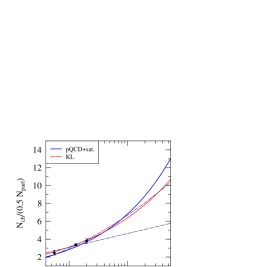
Figure 1: Multiplicity in the central unit of pseudorapidity. Data is from PHOBOS and dashed lines show the $\log(s)$ (straight) and $\log^{2}(s)$ (curved) growths.

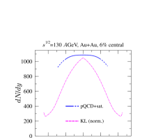
Figure 2: $dN/dy$ from the two saturation models. Normalization of the KL curve is such that after transforming, with an overall Jacobian factor, from $y$ to $\eta$ it agrees with data. Figure is from [5].

A crude estimate of $E_{\perp}$ in the pQCD+saturation model can be obtained from Eq.(6): at $\sqrt{s}=130$ GeV $E_{\perp}=520$ GeV and at $\sqrt{s}=200$ GeV $E_{\perp}=620$ GeV. Transverse expansion effects increase the above numbers a little [4]. PHENIX data at $\sqrt{s}=130$ is $E_{\perp}=578$ GeV [6].

The KL calculation has been shown to reproduce pseudorapidity distributions of hadrons at $\sqrt{s}=130$ GeV well [3]. From the theoretical point of view it is more instructive to look at the rapidity distributions of initial gluons, see Fig. 2. The pQCD+saturation model leads to a broad gaussian which, after transforming to pseudorapidity and comparing with data, overshoots at large rapidities. If saturation dynamics lead to flat $dN/dy$ near $y\sim 0$, this behaviour has to change around $y\sim y_{\rm{beam}}/2$ and the saturation dynamics must be replaced by some other fragmentation region dynamics. The KL result is qualitatively very different: it has a discontinuity in the first derivative of $dN/dy$ at $y=0$ and is exponentially suppressed away from it.

2.1 High Density QCD methods

The result of KL is based on the GLR equation [7]:

$$\frac{dN}{dy}=\frac{1}{\sigma_{\rm{in}}}\int dp_{\perp}^{2}\frac{\alpha}{p_{\perp}^{2}}\int^{p_{\perp}^{2}}dk_{\perp}^{2}\phi_{A}(x_{1},k_{\perp}^{2})\phi_{A}(x_{2},(p-k)_{\perp}^{2}),$$ (8)

which requires an ansatz for $\phi_{A}(x,k_{\perp}^{2})$. The ansatz used by KL is effectively

$$\phi_{A}(x,k_{\perp}^{2})=\frac{2}{3\pi^{2}}\frac{S_{A}}{\alpha}[\theta(Q_{s,A}^{2}-k_{\perp}^{2})+\epsilon\frac{Q_{s,A}^{2}}{k_{\perp}^{2}}\theta(k_{\perp}^{2}-Q_{s,A})],$$ (9)

where parametrically $\epsilon\sim O(\alpha^{2})$ and sets the relative normalization of the saturated and perturbative parts of the unintegrated gluon distribution. KL choose $\epsilon=0$ and regard the tail as a small correction. With ansatz (9) one obtains to leading logarithmic accuracy

$$\frac{dN}{dy}=\frac{2}{3\pi^{2}}\frac{S_{A}Q_{s,A}^{2}e^{-\lambda|y|}}{\alpha(Q_{s,A}^{2})}[2+2\lambda y(1+\epsilon)+2\epsilon[(1-\lambda)+\epsilon(1-\frac{3}{2}\lambda+\lambda y)].$$

Setting $\epsilon=0$ the KL result is reproduced. With $\epsilon=1$ and $\lambda=0.25$ one sees that the term $2\epsilon[\dots]$ originating entirely from the tail of the distribution and the first term from saturation region are roughly equal. For the transverse energy the tail is more important:

$$\frac{dE_{\perp}}{dy}=\frac{2}{3\pi^{2}}\frac{S_{A}Q_{s,A}^{3}e^{-3\lambda|y|/2}}{\alpha(Q_{s,A}^{2})}[\frac{4}{3}+2\lambda y(1+\epsilon)+4\epsilon[(1-2\lambda)+2\epsilon(1-\frac{7}{2}\lambda+\frac{\lambda}{2}y]].$$ (10)

Of course it is plausible that the relative normalization is not given by $\epsilon=1$ but by some smaller value, since $\epsilon\sim O(\alpha^{2})$, which would validate the exclusion of the tail.

2.2 Reshaping $dN/dy$

The ansatz (9) is probably too simple and one should try for example the one from [8]:

$$\phi_{A}(x,k_{\perp}^{2})\sim\int\frac{d^{2}z}{\alpha z^{2}}e^{-i{\bf{k\cdot z}}}(1-e^{-\frac{1}{4}Q_{s,A}^{2}(x)z^{2}\ln(z_{0}^{2}/z^{2}+1)}).$$ (11)

Using this in (8) one finds that the form of $dN/dy$ is

$$\frac{dN}{dy}\sim\frac{S_{A}Q_{s,A}^{2}}{\alpha(Q_{s,A})}\frac{\lambda y}{\sinh(\lambda y)}[6+\frac{1}{18}(2\lambda y)^{2}-\frac{1}{1800}(2\lambda y)^{4}+\dots].$$ (12)

This is very different from the one obtained with ansatz (9) and is closer to a broad gaussian as can be seen from the figure 4, which shows all of the discussed multiplicity distributions.

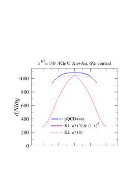
Figure 3: $dN/dy$ from the different calculations discussed in the text.

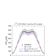
Figure 4: $dN/d\eta$ from the different calculations discussed in the text.

One needs also to take into account the large $x$ behaviour of the gluon distribution, $xG\sim(1-x)^{4}$, not contained in Eq.(11); whether this is sufficient to make agreement with data remains unclear at the moment. However near $y\sim 0$, one expects result (12) to be dominated by small $x$ part of $\phi_{A}$, and one might try to transform to pseudorapidity and compare with data. For KL this is done by an overall factor and for pQCD+saturation -model by assuming exponential $p_{\perp}$-spectra for pions. For details, see [3, 5]. From Fig. 4 one sees that the transformation of (12) with the overall factor leads to a very large dip around the central pseudorapidity. Hence, one should rather use the $p_{\perp}$-distributions to carry out the transformation. Probably the effects of the large $x$ behaviour of the gluon distribution should be included already at $y\sim 0$, too.

3 Conclusions

Particle production over the whole experimentally accessible rapidity range has been investigated using saturation models. While these models lead to very similar results at central unit of rapidity, they seem to differ at nonzero rapidities. This difference was suggested to originate from the choice for the unintegrated gluon structure function in the KL calculation, and a different ansatz was shown to lead to a gaussianlike distribution with a width comparable to the pQCD+saturation -model result. The quality of the approximations such as the neglect of the tail of the distributions and transformation from $y$ to $\eta$ with an overall Jacobian factor, was shown to be model dependent.

Acknowledgements: I would like to thank K.J. Eskola, K. Kajantie and P.V. Ruuskanen for collaboration and M. Gyulassy and D. Kharzeev for discussions.

References

- [1] K. Adcox et al., Phys. Rev. Lett. 86, 3500 (2001); C. Adler et al., Phys. Rev. Lett. 87, 112303 (2001); B.B. Back et al., Phys. Rev. Lett. 87, 102303 (2001), Phys. Rev. Lett. 88, 022302 (2002); I. G. Bearden et al., Phys. Lett. B 523, 227 (2001), Phys. Rev. Lett. 88, 202301 (2002).
- [2] K. J. Eskola, K. Kajantie, P. V. Ruuskanen and K. Tuominen, Nucl. Phys. B 570 (2000) 379.
- [3] D. Kharzeev and E. Levin, Phys. Lett. B 523 (2001) 79.
- [4] K. J. Eskola, P. V. Ruuskanen, S. S. Räsänen and K. Tuominen, Nucl. Phys. A 696 (2001) 715.
- [5] K. J. Eskola, K. Kajantie, P. V. Ruuskanen and K. Tuominen, hep-ph/0204034.
- [6] K. Adcox et al. Phys. Rev. Lett. 87 (2001) 052301.
- [7] L. V. Gribov, E. M. Levin and M. G. Ryskin, Phys. Rept. 100 (1983) 1.
- [8] E. Iancu, A. Leonidov and L. McLerran, hep-ph/0202270.