Analytical calculations of four-neutrino oscillations in matter

Abstract

We analytically derive transition probabilities for four-neutrino oscillations in matter. The time evolution operator giving the neutrino oscillations is expressed by the finite sum of terms up to the third power of the Hamiltonian in a matrix form, using the Cayley-Hamilton theorem. The result of computation for the probabilities in some mass patterns tells us that it is realistically difficult to observe the resonance between one of three active neutrinos and the fourth (sterile) neutrino near the earth, even if the fourth neutrino exists.

I Introduction

A neutrino oscillation is a transition among neutrino flavors. Several types of the observations tell us that neutrino oscillations occur [1, 2, 3, 4, 5, 6, 7, 8]. They are classified into the solar, atmospheric and LSND experiments.

The mass squared differences are the parameters showing the neutrino oscillations. In order to explain three kinds of neutrino experiments within one framework, three kinds of the mass squared differences are needed. Therefore we consider the four-neutrino oscillation, where the fourth neutrino doesn’t have the weak interaction. Three active neutrino flavors ($\nu_{e},\nu_{\mu},\nu_{\tau}$) interact with leptons in the weak interaction. So the fourth neutrino is called sterile neutrino ($\nu_{s}$).

The neutrino oscillation pattern in vacuum can get modified, when the neutrinos pass through matter. It is known as the Mikheyev-Smirnov-Wolfenstein (MSW) effect [9], which can be described by an effective Hamiltonian. The interaction with the neutral currents occurs for three active neutrinos. Thus, for the three active neutrinos, one doesn’t need to consider the interaction with the neutral currents [10]. But the sterile neutrino has neither the charged- nor the neutral-current interactions. It means that one needs to consider the effect of the matter interacting with the sterile neutrino and to introduce the $4\times 4$ mixing matrix of four neutrinos which is an extension of the $3\times 3$ Maki-Nakagawa-Sakata (MNS) matrix [11].

Analytical calculations of active three-neutrino oscillations in matter have been performed[12]. In this article, we derive analytically the transition probabilities for four-neutrino oscillations. Our calculations include the effects of the interaction with charged and neutral currents.

The outline of the article is as follows. In Sec. II, two kinds of the bases to express four-neutrino states are introduced. These bases are connected by a mixing matrix. To describe neutrino oscillations in matter, the effective Hamiltonian with charged and neutral current is introduced. In Sec. III, we calculate the transition probabilities from the effective Hamiltonian. In order to derive the transition probabilities, we make use of the Cayley-Hamilton theorem and the formula for the root of biquadratic equation. In Sec. IV, the transition probabilities are concretely computed in two cases of the four-neutrino oscillation schemes. Finally, in Sec. V, we discuss the effects of four-neutrino oscillations in matter.

II Formalism

A Two bases and a mixing matrix

Neutrinos are produced in flavor eigenstates $|{\nu_{\alpha}}\rangle(\alpha=e,\mu,\tau,s)$. Between the source and the detector, the neutrinos evolve as mass eigenstates $|{\nu_{a}}\rangle(a=1,2,3,4)$. There are two kinds of eigenstates: $|{\nu_{\alpha}}\rangle$ and $|{\nu_{a}}\rangle$. These eigenstates are defined by neutrino fields $\nu_{\alpha}$ and $\nu_{a}$ corresponding to each eigenstate: $\nu^{\dagger}|{0}\rangle\equiv|{\nu}\rangle$, $|{\nu_{\alpha}}\rangle\equiv|{\alpha}\rangle$, $|{\nu_{a}}\rangle\equiv|{a}\rangle$, where a vacuum state is given by $|{0}\rangle$. In the present analysis, we will use the plane wave approximation of the fields. In this approximation, a neutrino flavor field $\nu_{\alpha}$ is expressed by a linear combination of neutrino mass field $\nu_{a}$:

$$\nu_{\alpha}=\sum_{a=1}^{4}U_{\alpha a}\nu_{a},$$ (1)

where $U$ is a 4 $\times$ 4 unitary matrix with the elements $U_{\alpha a}$. If we write this relation in neutrino eigenstates, then

$$|{\alpha}\rangle=\sum_{a=1}^{4}U_{\alpha a}^{*}|{a}\rangle.$$ (2)

An arbitrary neutrino state $\psi$ is expressed in both the flavor and mass bases as

$$\psi\equiv\sum_{\alpha=e,\mu,\tau,s}\psi_{\alpha}|{\alpha}\rangle=\sum_{\alpha=e,\mu,\tau,s}\psi_{\alpha}\sum_{a=1}^{4}U_{\alpha a}^{*}|{a}\rangle=\sum_{a=1}^{4}\left(\sum_{\alpha=e,\mu,\tau,s}\psi_{\alpha}U_{\alpha a}^{*}\right)|{a}\rangle=\sum_{a=1}^{4}\psi_{a}|{a}\rangle,$$ (3)

where $\psi_{\alpha}$ and $\psi_{a}$ are the components of $\psi$ of the flavor eigenstate basis and the mass eigenstate basis, respectively. They are related to each other in the form with respect to

$$\psi_{a}=\sum_{\alpha=e,\mu,\tau,s}U_{\alpha a}^{*}\psi_{\alpha}.$$ (4)

If we define the matrix elements as

$$\psi_{f} = (\psi_{\alpha})=\left(\begin{array}[]{c}\psi_{e}\\ \psi_{\mu}\\ \psi_{\tau}\\ \psi_{s}\end{array}\right),\quad\psi_{m}=(\psi_{a})=\left(\begin{array}[]{c}\psi_{1}\\ \psi_{2}\\ \psi_{3}\\ \psi_{4}\end{array}\right),$$ (13)

$$U = (U_{\alpha a})=\left(\begin{array}[]{cccc}U_{e1}&U_{e2}&U_{e3}&U_{e4}\\ U_{\mu 1}&U_{\mu 2}&U_{\mu 3}&U_{\mu 4}\\ U_{\tau 1}&U_{\tau 2}&U_{\tau 3}&U_{\tau 4}\\ U_{s1}&U_{s2}&U_{s3}&U_{s4}\end{array}\right),$$ (18)

the relation between the flavor and the mass eigenstates are

$$\left(\begin{array}[]{c}\nu_{e}\\ \nu_{\mu}\\ \nu_{\tau}\\ \nu_{s}\end{array}\right)=\left(\begin{array}[]{cccc}U_{e1}&U_{e2}&U_{e3}&{U_{e4}}\\ U_{\mu 1}&U_{\mu 2}&U_{\mu 3}&{U_{\mu 4}}\\ U_{\tau 1}&U_{\tau 2}&U_{\tau 3}&{U_{\tau 4}}\\ {U_{s1}}&{U_{s2}}&{U_{s3}}&{U_{s4}}\end{array}\right)\left(\begin{array}[]{c}\nu_{1}\\ \nu_{2}\\ \nu_{3}\\ \nu_{4}\end{array}\right).$$ (19)

The unitary matrix $U$ is the mixing matrix of four neutrinos. There are 6 mixing angles and 3 mixing phases as parameters of $U$, in the case of 4 neutrinos. In this analysis, we ignore the CP violation by putting the mixing phases equal to zero. Then, $U$ is the real orthogonal matrix[12].

A parameterization for $U=U(\theta_{12},\theta_{13},\theta_{14},\theta_{23},\theta_{24},\theta_{34})$ is given by

$$U=U_{34}U_{24}U_{14}U_{23}U_{13}U_{12},$$ (20)

where matrix elements are

$${\left(U_{ij}\right)}_{ab}=\delta_{ab}+(C_{ij}-1)(\delta_{ia}\delta_{ib}+\delta_{ja}\delta_{jb})+S_{ij}(\delta_{ia}\delta_{jb}-\delta_{ja}\delta_{ib}),$$ (21)

$$C_{ij}=\cos\theta_{ij},\quad S_{ij}=\sin\theta_{ij},$$ (22)

and the mixing angles $\theta_{12},\theta_{13},\theta_{14},\theta_{23},\theta_{24},\theta_{34}$ [13, 14]. By this definition, the mixing matrix becomes

$$U=$$ (23)

$$\left(\begin{array}[]{llll}\begin{array}[]{l}C_{12}C_{13}C_{14}\\ \\ \end{array}&\begin{array}[]{l}C_{13}C_{14}S_{12}\\ \\ \end{array}&\begin{array}[]{l}C_{14}S_{13}\\ \\ \end{array}&\begin{array}[]{l}S_{14}\\ \\ \end{array}\\ \begin{array}[]{l}-C_{23}C_{24}S_{12}\\ -C_{12}C_{24}S_{13}S_{23}\\ -C_{12}C_{13}S_{14}S_{24}\\ \\ \end{array}&\begin{array}[]{l}C_{12}C_{23}C_{24}\\ -C_{24}S_{12}S_{13}S_{23}\\ -C_{13}S_{12}S_{14}S_{24}\\ \\ \end{array}&\begin{array}[]{l}C_{13}C_{24}S_{23}\\ -S_{13}S_{14}S_{24}\\ \\ \end{array}&\begin{array}[]{l}C_{14}S_{24}\\ \\ \end{array}\\ \begin{array}[]{l}-C_{12}C_{23}C_{34}S_{13}\\ +C_{34}S_{12}S_{23}\\ -C_{12}C_{13}C_{24}S_{14}S_{34}\\ +C_{23}S_{12}S_{24}S_{34}\\ +C_{12}S_{13}S_{23}S_{24}S_{34}\\ \\ \end{array}&\begin{array}[]{l}-C_{23}C_{34}S_{12}S_{13}\\ -C_{12}C_{34}S_{23}\\ -C_{13}C_{24}S_{12}S_{14}S_{34}\\ -C_{12}C_{23}S_{24}S_{34}\\ +S_{12}S_{13}S_{23}S_{24}S_{34}\\ \\ \end{array}&\begin{array}[]{l}C_{13}C_{23}C_{34}\\ -C_{24}S_{13}S_{14}S_{34}\\ -C_{13}S_{23}S_{24}S_{34}\\ \\ \end{array}&\begin{array}[]{l}C_{14}C_{24}S_{34}\\ \\ \end{array}\\ \begin{array}[]{l}-C_{12}C_{13}C_{24}C_{34}S_{14}\\ +C_{23}C_{34}S_{12}S_{24}\\ +C_{12}C_{34}S_{13}S_{23}S_{24}\\ +C_{12}C_{23}S_{13}S_{34}\\ -S_{12}S_{23}S_{34}\\ \\ \end{array}&\begin{array}[]{l}-C_{13}C_{24}C_{34}S_{12}S_{14}\\ -C_{12}C_{23}C_{34}S_{24}\\ +C_{34}S_{12}S_{13}S_{23}S_{24}\\ +C_{23}S_{12}S_{13}S_{34}\\ +C_{12}S_{23}S_{34}\\ \\ \end{array}&\begin{array}[]{l}-C_{24}C_{34}S_{13}S_{14}\\ -C_{13}C_{34}S_{23}S_{24}\\ -C_{13}C_{23}S_{34}\\ \end{array}&\begin{array}[]{l}C_{14}C_{24}C_{34}\\ \end{array}\\ \end{array}\right).$$ (83)

B Hamiltonian in matter

In the mass eigenstate basis, the Hamiltonian ${\mathcal{H}}_{0}$ participating in the propagation of neutrinos in vacuum is given by

$${\mathcal{H}}_{0}=\left(\begin{array}[]{cccc}E_{1}&0&0&0\\ 0&E_{2}&0&0\\ 0&0&E_{3}&0\\ 0&0&0&E_{4}\\ \end{array}\right),$$ (84)

where $E_{a}~{}(a=1,2,3,4)$ are the energies of the neutrino mass eigenstates $|{a}\rangle$ with mass $m_{a}$:

$$E_{a}=\sqrt{{m_{a}}^{2}+\bm{p}^{2}}.$$ (85)

Here and hereafter we assume the momentum $\bm{p}$ to be the same for all mass eigenstates.

There are two kinds of the additional potentials for describing the interactions between neutrinos and matter. One is the interaction of the charged particles (electrons) and its neutrino $\nu_{e}$:

$$V_{e}=\sqrt{2}G_{F}~{}\text{diag}(N_{e},0,0,0).$$ (86)

The other is the interaction of the neutral particles(e.g. the neutron) and active neutrinos ($\nu_{e},\nu_{\mu},\nu_{\tau}$):

$$V_{n0}=\sqrt{2}G_{F}~{}\text{diag}(-\frac{1}{2}N_{n},-\frac{1}{2}N_{n},-\frac{1}{2}N_{n},0),$$ (87)

where $G_{F}$, $N_{e}$ and $N_{n}$ are the Fermi weak coupling constant, the electron number density and the neutral particle number density, respectively. Note that we assume the particle number densities to be constant throughout the matter where the neutrinos are propagating.

The interaction term (87) can be separated into two parts as

$$V_{n0} = V_{n}+V^{\prime},$$ (88)

$$V_{n} = \sqrt{2}G_{F}~{}\text{diag}(0,0,0,+\frac{1}{2}N_{n}),$$ (89)

$$V^{\prime} = \sqrt{2}G_{F}~{}\text{diag}(-\frac{1}{2}N_{n},-\frac{1}{2}N_{n},-\frac{1}{2}N_{n},-\frac{1}{2}N_{n}).$$ (90)

These interaction terms are written by the flavor eigenstate basis. Therefore the interaction terms in the flavor eigenstate basis must be transformed into those in the mass eigenstate basis by the mixing matrix $U$. The interaction terms in the mass eigenstate basis are

$$U^{-1}V_{e}U = A_{e}\left(\begin{array}[]{cccc}U_{e1}^{2}&U_{e1}U_{e2}&U_{e1}U_{e3}&U_{e1}U_{e4}\\ U_{e2}U_{e1}&U_{e2}^{2}&U_{e2}U_{e3}&U_{e2}U_{e4}\\ U_{e3}U_{e1}&U_{e3}U_{e2}&U_{e3}^{2}&U_{e3}U_{e4}\\ U_{e4}U_{e1}&U_{e4}U_{e2}&U_{e4}U_{e3}&U_{e4}^{2}\\ \end{array}\right),$$ (95)

$$U^{-1}V_{n}U = A_{n}\left(\begin{array}[]{cccc}U_{s1}^{2}&U_{s1}U_{s2}&U_{s1}U_{s3}&U_{s1}U_{s4}\\ U_{s2}U_{s1}&U_{s2}^{2}&U_{s2}U_{s3}&U_{s2}U_{s4}\\ U_{s3}U_{s1}&U_{s3}U_{s2}&U_{s3}^{2}&U_{s3}U_{s4}\\ U_{s4}U_{s1}&U_{s4}U_{s2}&U_{s4}U_{s3}&U_{s4}^{2}\\ \end{array}\right),$$ (100)

$$U^{-1}V^{\prime}U = -A_{n}I,$$ (101)

where $I$ is the $4\times 4$ unit matrix, and the matter densities $A_{e},A_{n}$ and $A$ are defined by

$$A_{e} = \sqrt{2}G_{F}N_{e}\equiv A,$$ (102)

$$A_{n} = \frac{1}{\sqrt{2}}G_{F}N_{n}=\frac{1}{2}A\frac{N_{n}}{N_{e}}.$$ (103)

Thus, the Hamiltonian in the case when the neutrinos propagate in matter is

$${\mathcal{H}}_{m}={\mathcal{H}}_{0}+U^{-1}V_{e}U+U^{-1}V_{n}U-A_{n}I.$$ (104)

III Calculations of the neutrino transition probabilities

The transition probabilities are represented by the time evolution operator. In the flavor state basis, the unitary transformation from the initial state $\psi_{f}(t=0)$ to the final state $\psi_{f}(t)$ is given by the operator

$$U_{f}(t)\equiv U_{f}(t,0),$$ (105)

where $U_{f}(t_{2},t_{1})$ is the time evolution operator from time $t_{1}$ to $t_{2}$ in the flavor state basis. The Hamiltonian ${\mathcal{H}}_{\textrm{flavor}}$ in the flavor state basis is represented by using the mixing matrix $U$ and the Hamiltonian ${\mathcal{H}}_{m}$ in the mass state basis:

$${\mathcal{H}}_{\textrm{flavor}}=U{\mathcal{H}}_{m}U^{-1}.$$ (106)

The Schrödinger equation in the mass eigenstate basis is

$$i\frac{d}{dt}\psi_{m}(t)={\mathcal{H}}_{m}\psi_{m}(t).$$ (107)

Equation (107) has a solution

$$\psi_{m}(t)=e^{-i{\mathcal{H}}_{m}t}\psi_{m}(0),$$ (108)

where $e^{-i{\mathcal{H}}_{m}t}$ is the time evolution operator. Inserting $t=L$ into (108), the solution of the Schrödinger equation (107) is

$$\psi_{m}(L)=\psi_{m}(t)\Big{|}_{t=L}=e^{-i{\mathcal{H}}_{m}L}\psi_{m}(0)\equiv U_{m}(L)\psi_{m}(0),$$ (109)

where $L$ stands for the distance through which neutrinos run for the time $t$, because the speed of neutrinos is almost equal to that of light.

The neutrino state $\psi_{f}(L)$ at $t=L$ in the flavor state basis is expressed as

$$\psi_{f}(L)=U\psi_{m}(L)=Ue^{-i{\mathcal{H}}_{m}L}\psi_{m}(0)=Ue^{-i{\mathcal{H}}_{m}L}U^{-1}\psi_{f}(0)\equiv U_{f}(L)\psi_{f}(0).$$ (110)

A Traceless matrix $T$

In order to find the explicit form of the time evolution operator $e^{-i{\mathcal{H}}_{m}t}$, which is the exponential of the matrix, the Hamiltonian in the matrix form is separated into the diagonal and the traceless matrices. The trace of the matrix ${\mathcal{H}}_{m}$ in (104) is

$${\mathrm{tr}}{\mathcal{H}}_{m}=E_{1}+E_{2}+E_{3}+E_{4}+A_{e}-3A_{n},$$ (111)

where we use the unitarity conditions, e.g. ${U_{e1}}^{2}+{U_{e2}}^{2}+{U_{e3}}^{2}+{U_{e4}}^{2}=1$.

An arbitrary $N\times N$ matrix $M$ can always be written as

$$M=M_{0}+\frac{1}{N}({\mathrm{tr}}M)I_{N},$$ (112)

where $M_{0}$ and $I_{N}$ are $N\times N$ traceless and unit matrices, respectively. Note that ${\mathrm{tr}}M_{0}=0$. Then the $4\times 4$ matrix ${\mathcal{H}}_{m}$ can be written as

$${\mathcal{H}}_{m}=T+\frac{1}{4}({\mathrm{tr}}{\mathcal{H}}_{m})I,$$ (113)

where $I_{4}=I$ and the matrix $T$ is traceless. The matrix $T$ can be written by

$$T = {\mathcal{H}}_{0}-\frac{1}{4}(E_{1}+E_{2}+E_{3}+E_{4})I+U^{-1}V_{e}U+U^{-1}V_{n}U-\frac{1}{4}(A_{e}+A_{n})I$$ (114)

$$= \frac{1}{4}\left(\begin{array}[]{cccc}E_{1,234}&0&0&0\\ 0&E_{2,134}&0&0\\ 0&0&E_{3,124}&0\\ 0&0&0&E_{4,123}\\ \end{array}\right)$$ (129)

$$+A_{e}\left(\begin{array}[]{cccc}{U_{e1}}^{2}-\frac{1}{4}&{U_{e1}}{U_{e2}}&{U_{e1}}{U_{e3}}&{U_{e1}}{U_{e4}}\\ {U_{e2}}{U_{e1}}&{U_{e2}}^{2}-\frac{1}{4}&{U_{e2}}{U_{e3}}&{U_{e2}}{U_{e4}}\\ {U_{e3}}{U_{e1}}&{U_{e3}}{U_{e2}}&{U_{e3}}^{2}-\frac{1}{4}&{U_{e3}}{U_{e4}}\\ {U_{e4}}{U_{e1}}&{U_{e4}}{U_{e2}}&{U_{e4}}{U_{e3}}&{U_{e4}}^{2}-\frac{1}{4}\\ \end{array}\right)$$

$$+A_{n}\left(\begin{array}[]{cccc}{U_{s1}}^{2}-\frac{1}{4}&{U_{s1}}{U_{s2}}&{U_{s1}}{U_{s3}}&{U_{s1}}{U_{s4}}\\ {U_{s2}}{U_{s1}}&{U_{s2}}^{2}-\frac{1}{4}&{U_{s2}}{U_{s3}}&{U_{s2}}{U_{s4}}\\ {U_{s3}}{U_{s1}}&{U_{s3}}{U_{s2}}&{U_{s3}}^{2}-\frac{1}{4}&{U_{s3}}{U_{s4}}\\ {U_{s4}}{U_{s1}}&{U_{s4}}{U_{s2}}&{U_{s4}}{U_{s3}}&{U_{s4}}^{2}-\frac{1}{4}\\ \end{array}\right),$$

where $E_{ab}~{}(a,b=1,2,3,4,a\neq b)$ and $E_{k,lmn}(k,l,m,n=1,2,3,4)$ are defined as

$$E_{ab}\equiv E_{a}-E_{b},\quad E_{k,lmn}\equiv E_{kl}+E_{km}+E_{kn},$$ (130)

respectively. The energy differences $E_{ab}$ are not linearly independent, since they obey the following relations:

$$E_{ab}=-E_{ba},\quad E_{12}+E_{23}+E_{31}=0,\quad E_{12}+E_{24}+E_{41}=0,\quad E_{13}+E_{34}+E_{41}=0.$$

Thus, only three of the $E_{ab}$’s are linearly independent.

Therefore the time evolution operator $e^{-i{\mathcal{H}}_{m}t}$ can be rewritten by the traceless matrix $T$:

$$U_{m}(L)=e^{-i{\mathcal{H}}_{m}L}=\phi e^{-iTL},$$ (131)

where $\phi=e^{-{i}({\mathrm{tr}}{\mathcal{H}}_{m})L/4}$ is a phase factor.

B The Cayley-Hamilton theorem

In order to find the concrete form of the definite matrix $e^{-iTL}$, we use the Cayley-Hamilton theorem. The exponential of the $4\times 4$ matrix $T$ can be expressed by an infinite series

$$e^{-iTL}=k_{0}I+k_{1}T+k_{2}T^{2}+k_{3}T^{3}+k_{4}T^{4}+\cdots,$$ (132)

where $k_{n}=\frac{{(-iL)}^{n}}{n!}\quad(n=1,2,3,4,\cdots)$. The Cayley-Hamilton theorem implies that the eigenvalue $\lambda$ in the characteristic equation

$${\mathrm{det}}(T-\lambda I_{4})={\lambda}^{4}+c_{3}{\lambda}^{3}+c_{2}{\lambda}^{2}+c_{1}{\lambda}+c_{0}=0$$ (133)

of the matrix $T$ can be replaced with $T$ to give

$${T}^{4}+c_{3}{T}^{3}+c_{2}{T}^{2}+c_{1}{T}+c_{0}=0,$$ (134)

where $c_{j}$ $(j=0,1,2,3)$ are coefficients. Using (134) repeatedly, the matrix $e^{-iTL}$ can be formally written in the form

$$e^{-iTL}=a_{0}I+a_{1}T+a_{2}T^{2}+a_{3}T^{3},$$ (135)

where $a_{j}$ $(j=0,1,2,3)$ are coefficients which differ from $k_{n}$ and $c_{j}$ in general.

Because $T$ is the definite matrix, we need to find the coefficients $a_{j}$ explicitly in order to obtain the matrix $e^{-iTL}$. If the characteristic equation (133) has four solutions $\lambda_{k}$ $(k=1,2,3,4)$, one can write the eigenvalues of $e^{-iTL}$ as

$$e^{-i{\lambda_{k}}L}=a_{0}+a_{1}{\lambda_{k}}+a_{2}{\lambda_{k}}^{2}+a_{3}{\lambda_{k}}^{3}.$$ (136)

By defining the following matrices,

$$\bm{e}=\left(\begin{array}[]{c}e^{-iL\lambda_{1}}\\ e^{-iL\lambda_{2}}\\ e^{-iL\lambda_{3}}\\ e^{-iL\lambda_{4}}\end{array}\right),\quad\Lambda=\left(\begin{array}[]{cccc}1&-iL{\lambda_{1}}&-L^{2}{\lambda_{1}}^{2}&+iL^{3}{\lambda_{1}}^{3}\\ 1&-iL{\lambda_{2}}&-L^{2}{\lambda_{2}}^{2}&+iL^{3}{\lambda_{2}}^{3}\\ 1&-iL{\lambda_{3}}&-L^{2}{\lambda_{3}}^{2}&+iL^{3}{\lambda_{3}}^{3}\\ 1&-iL{\lambda_{4}}&-L^{2}{\lambda_{4}}^{2}&+iL^{3}{\lambda_{4}}^{3}\end{array}\right),\quad\bm{a}=\left(\begin{array}[]{c}a_{0}\\ a_{1}\\ a_{2}\\ a_{3}\\ \end{array}\right),$$ (149)

(136) is written as the matrix form $\bm{e}=\Lambda\bm{a}$. Then, one obtain the coefficient $\bm{a}$ by

$$\bm{a}=\Lambda^{-1}\bm{e}.$$ (150)

Therefore, we should find the eigenvalues $\lambda_{k}$ of the matrix $T$ in order to know $\bm{a}$.

C Characteristic equation of the matrix $T$

In order to obtain the eigenvalues $\lambda_{k}$ of the matrix $T$, one must solve the characteristic equation

$$\left|\begin{array}[]{cccc}T_{11}-\lambda&T_{12}&T_{13}&T_{14}\\ T_{21}&T_{22}-\lambda&T_{23}&T_{24}\\ T_{31}&T_{32}&T_{33}-\lambda&T_{34}\\ T_{41}&T_{42}&T_{43}&T_{44}-\lambda\end{array}\right|={\lambda}^{4}+c_{3}{\lambda}^{3}+c_{2}{\lambda}^{2}+c_{1}{\lambda}+c_{0}=0.$$ (151)

The coefficient $c_{0}$ is the determinant of $T$, $c_{1}$ and $c_{2}$ are expressed by the sum of cofactors of $T$, and $c_{3}$ is given by the trace of $T$,

$$c_{3} = -(T_{11}+T_{22}+T_{33}+T_{44})=-{\mathrm{tr}}T=0,$$

$$c_{2} = +T_{11}T_{22}+T_{11}T_{33}+T_{11}T_{44}+T_{22}T_{33}+T_{22}T_{44}+T_{33}T_{44}$$

$$-T_{12}T_{21}-T_{13}T_{31}-T_{14}T_{41}-T_{23}T_{32}-T_{24}T_{42}-T_{34}T_{43},$$

$$c_{1} = -T_{11}T_{22}T_{33}-T_{11}T_{22}T_{44}-T_{11}T_{33}T_{44}-T_{22}T_{33}T_{44}$$

$$+T_{11}T_{23}T_{32}+T_{11}T_{24}T_{42}+T_{11}T_{34}T_{43}+T_{22}T_{13}T_{31}+T_{22}T_{14}T_{41}+T_{22}T_{34}T_{43}$$

$$+T_{33}T_{12}T_{21}+T_{33}T_{14}T_{41}+T_{33}T_{24}T_{42}+T_{44}T_{12}T_{21}+T_{44}T_{13}T_{31}+T_{44}T_{23}T_{32}$$

$$-T_{13}T_{34}T_{41}-T_{14}T_{43}T_{31}-T_{12}T_{24}T_{41}-T_{14}T_{42}T_{21}$$

$$-T_{12}T_{23}T_{31}-T_{13}T_{32}T_{21}-T_{23}T_{34}T_{42}-T_{24}T_{43}T_{32},$$

$$c_{0} = T_{11}T_{22}T_{33}T_{44}$$

$$-T_{11}T_{22}T_{34}T_{43}-T_{11}T_{33}T_{24}T_{42}-T_{11}T_{44}T_{23}T_{32}$$

$$-T_{22}T_{33}T_{14}T_{41}-T_{22}T_{44}T_{13}T_{31}-T_{33}T_{44}T_{12}T_{21}$$

$$+T_{11}T_{23}T_{34}T_{42}+T_{11}T_{24}T_{43}T_{32}+T_{22}T_{13}T_{34}T_{41}+T_{22}T_{14}T_{43}T_{31}$$

$$+T_{33}T_{12}T_{24}T_{41}+T_{33}T_{14}T_{42}T_{21}+T_{44}T_{12}T_{23}T_{31}+T_{44}T_{13}T_{32}T_{21}$$

$$-T_{12}T_{23}T_{34}T_{41}-T_{12}T_{24}T_{43}T_{31}-T_{13}T_{32}T_{24}T_{41}$$

$$-T_{13}T_{34}T_{42}T_{21}-T_{14}T_{42}T_{23}T_{31}-T_{14}T_{43}T_{32}T_{21}$$

$$+T_{12}T_{21}T_{34}T_{43}+T_{13}T_{31}T_{24}T_{42}+T_{14}T_{41}T_{23}T_{32}.$$

The four roots of the biquadratic equation (151) are given from the solutions of the two quadratic equations [15]

$$X^{2}\pm\sqrt{t_{0}-c_{2}}X+\frac{t_{0}}{2}+\sqrt{{\frac{t_{0}}{2}}^{2}-c_{0}}=0,$$ (152)

where $t_{0}$ is one of real roots of the cubic equation

$$t^{3}-c_{2}t^{2}-4c_{0}t+4c_{0}c_{2}-{c_{1}}^{2}=0.$$ (153)

Note that $c_{3}=-{\mathrm{tr}}T=0$ due to the definition of $T$.

D Calculation of time evolution operator

From (131) and (135), the time evolution operator is written as

$$U_{m}(L) = e^{-i{\mathcal{H}}_{m}L}=\phi e^{-iTL}$$ (154)

$$= \phi\left[a_{0}I+(-iLT)a_{1}-L^{2}T^{2}a_{2}+iL^{3}T^{3}a_{3}\right].$$ (155)

The coefficients $a_{j}$’s are given by (150) as follows,

$$a_{0} = -\frac{\lambda_{2}\lambda_{3}\lambda_{4}}{\lambda_{12}\lambda_{13}\lambda_{14}}e^{-iL\lambda_{1}}-\frac{\lambda_{1}\lambda_{3}\lambda_{4}}{\lambda_{21}\lambda_{23}\lambda_{24}}e^{-iL\lambda_{2}}-\frac{\lambda_{1}\lambda_{2}\lambda_{4}}{\lambda_{31}\lambda_{32}\lambda_{34}}e^{-iL\lambda_{3}}-\frac{\lambda_{1}\lambda_{2}\lambda_{3}}{\lambda_{41}\lambda_{42}\lambda_{43}}e^{-iL\lambda_{4}},$$

$$a_{1} = \frac{i}{L}\left(\frac{\lambda_{2}\lambda_{3}+\lambda_{2}\lambda_{4}+\lambda_{3}\lambda_{4}}{\lambda_{12}\lambda_{13}\lambda_{14}}e^{-iL\lambda_{1}}+\frac{\lambda_{1}\lambda_{3}+\lambda_{1}\lambda_{4}+\lambda_{3}\lambda_{4}}{\lambda_{21}\lambda_{23}\lambda_{24}}e^{-iL\lambda_{2}}\right.$$

$$\left.+\frac{\lambda_{1}\lambda_{2}+\lambda_{1}\lambda_{4}+\lambda_{2}\lambda_{4}}{\lambda_{31}\lambda_{32}\lambda_{34}}e^{-iL\lambda_{3}}+\frac{\lambda_{1}\lambda_{2}+\lambda_{1}\lambda_{3}+\lambda_{2}\lambda_{3}}{\lambda_{41}\lambda_{42}\lambda_{43}}e^{-iL\lambda_{4}}\right),$$

$$a_{2} = \frac{1}{L^{2}}\left(\frac{\lambda_{2}+\lambda_{3}+\lambda_{4}}{\lambda_{12}\lambda_{13}\lambda_{14}}e^{-iL\lambda_{1}}+\frac{\lambda_{1}+\lambda_{3}+\lambda_{4}}{\lambda_{21}\lambda_{23}\lambda_{24}}e^{-iL\lambda_{2}}\right.$$

$$\left.+\frac{\lambda_{1}+\lambda_{2}+\lambda_{4}}{\lambda_{31}\lambda_{32}\lambda_{34}}e^{-iL\lambda_{3}}+\frac{\lambda_{1}+\lambda_{2}+\lambda_{3}}{\lambda_{41}\lambda_{42}\lambda_{43}}e^{-iL\lambda_{4}}\right),$$

$$a_{3} = \frac{-i}{L^{3}}\left(\frac{1}{\lambda_{12}\lambda_{13}\lambda_{14}}e^{-iL\lambda_{1}}+\frac{1}{\lambda_{21}\lambda_{23}\lambda_{24}}e^{-iL\lambda_{2}}+\frac{1}{\lambda_{31}\lambda_{32}\lambda_{34}}e^{-iL\lambda_{3}}+\frac{1}{\lambda_{41}\lambda_{42}\lambda_{43}}e^{-iL\lambda_{4}}\right),$$

where $\lambda_{ab}\equiv\lambda_{a}-\lambda_{b}$. Inserting these results into (155), one can find the time evolution operator in terms of $\lambda_{a}$’s. For example, the term containing $e^{-iL\lambda_{1}}$ is

$$-\frac{\lambda_{2}\lambda_{3}\lambda_{4}I-(\lambda_{2}\lambda_{3}+\lambda_{2}\lambda_{4}+\lambda_{3}\lambda_{4})T+(\lambda_{2}+\lambda_{3}+\lambda_{4})T^{2}-T^{3}}{{\lambda_{1}}^{3}-(\lambda_{2}+\lambda_{3}+\lambda_{4}){\lambda_{1}}^{2}-(\lambda_{2}\lambda_{3}+\lambda_{2}\lambda_{4}+\lambda_{3}\lambda_{4})\lambda_{1}-\lambda_{2}\lambda_{3}\lambda_{4}}e^{-iL\lambda_{1}}.$$ (156)

Using the relations of the coefficients and solutions for the biquadratic equations,

$$\lambda_{1}+\lambda_{2}+\lambda_{3}+\lambda_{4} = -c_{3}=0,$$ (157)

$$\lambda_{1}\lambda_{2}+\lambda_{2}\lambda_{3}+\lambda_{3}\lambda_{4}+\lambda_{4}\lambda_{1}+\lambda_{1}\lambda_{3}+\lambda_{2}\lambda_{4} = c_{2},$$ (158)

$$\lambda_{1}\lambda_{2}\lambda_{3}+\lambda_{2}\lambda_{3}\lambda_{4}+\lambda_{1}\lambda_{2}\lambda_{4}+\lambda_{1}\lambda_{3}\lambda_{4} = -c_{1},$$ (159)

$$\lambda_{1}\lambda_{2}\lambda_{3}\lambda_{4} = c_{0},$$ (160)

(156) can be written as

$$\frac{(c_{1}+c_{2}\lambda_{1}+{\lambda_{1}}^{3})I+(c_{2}+{\lambda_{1}}^{2})T+{\lambda_{1}}T^{2}+T^{3}}{4{\lambda_{1}}^{3}+c_{1}+2c_{2}\lambda_{1}}e^{-iL\lambda_{1}}.$$ (161)

Therefore, the matrix $e^{-iTL}$ is given by

$$e^{-iTL} = \sum_{a=1}^{4}B_{a}e^{-iL\lambda_{a}},$$ (162)

$$B_{a} \equiv \frac{(c_{1}+c_{2}\lambda_{a}+{\lambda_{a}}^{3})I+(c_{2}+{\lambda_{a}}^{2})T+{\lambda_{a}}T^{2}+T^{3}}{4{\lambda_{a}}^{3}+c_{1}+2c_{2}\lambda_{a}}.$$ (163)

The time evolution operator in the mass eigenstate is derived by

$$U_{m}(L)=e^{-i{\mathcal{H}}_{m}L}=\phi\sum_{a=1}^{4}B_{a}e^{-iL\lambda_{a}}.$$ (164)

Using the mixing matrix $U$, the time evolution operator in the flavor eigenstate is given as

$$U_{f}(L) = e^{-i{\mathcal{H}}_{f}L}=Ue^{-i{\mathcal{H}}_{m}L}U^{-1}=\phi\sum_{a=1}^{4}\tilde{B_{a}}e^{-iL\lambda_{a}},$$ (165)

$$\tilde{B_{a}} \equiv U{B_{a}}U^{-1}=\frac{(c_{1}+c_{2}\lambda_{a}+{\lambda_{a}}^{3})I+(c_{2}+{\lambda_{a}}^{2})\tilde{T}+{\lambda_{a}}\tilde{T}^{2}+\tilde{T}^{3}}{4{\lambda_{a}}^{3}+c_{1}+2c_{2}\lambda_{a}},$$ (166)

where $\tilde{T}\equiv UTU^{-1}$.

E Transition probabilities in matter

A probability amplitude is defined as

$$A_{\alpha\beta}\equiv\langle{\beta}|U_{f}(L)|{\alpha}\rangle,\quad\alpha,\beta=e,\mu,\tau,s.$$ (167)

Inserting (165) into (167) the probability amplitude becomes

$$A_{\alpha\beta} = \phi\sum_{a=1}^{4}\tilde{(B_{a})}_{\alpha\beta}e^{-iL\lambda_{a}},$$ (168)

$$\tilde{(B_{a})}_{\alpha\beta} = \frac{(c_{1}+c_{2}\lambda_{a}+{\lambda_{a}}^{3})\delta_{\alpha\beta}+(c_{2}+{\lambda_{a}}^{2}){\tilde{T}}_{\alpha\beta}+{\lambda_{a}}^{2}{(\tilde{T}^{2})}_{\alpha\beta}+{(\tilde{T}^{3})}_{\alpha\beta}}{4{\lambda_{a}}^{3}+c_{1}+2c_{2}\lambda_{a}},$$ (169)

where

$$\langle{\alpha}|I|{\beta}\rangle=\delta_{\alpha\beta},\quad\langle{\alpha}|\tilde{T}|{\beta}\rangle=\tilde{T}_{\alpha\beta},\quad\langle{\alpha}|{\tilde{T}}^{2}|{\beta}\rangle={({\tilde{T}}^{2})}_{\alpha\beta},\quad\langle{\alpha}|{\tilde{T}}^{3}|{\beta}\rangle={({\tilde{T}}^{3})}_{\alpha\beta}.$$ (170)

Here $\delta_{\alpha\beta}$, $\tilde{T}_{\alpha\beta}$, ${({\tilde{T}}^{2})}_{\alpha\beta}$ and ${({\tilde{T}}^{3})}_{\alpha\beta}$ are all symmetric. The probability of transition from the neutrino flavor $\alpha$ to the neutrino flavor $\beta$ is defined by

$$P_{\alpha\beta}\equiv\left|A_{\alpha\beta}\right|^{2}={A_{\alpha\beta}}^{*}A_{\alpha\beta}.$$ (171)

Using the definition of the probability amplitude (167), one finds

$$P_{\alpha\beta}=\sum_{a=1}^{4}\sum_{b=1}^{4}\tilde{(B_{a})}_{\alpha\beta}\tilde{(B_{b})}_{\alpha\beta}e^{-iL(\lambda_{a}-\lambda_{b})},$$ (172)

where the symmetry of $T$ leads $P_{\alpha\beta}=P_{\beta\alpha}$.

The probabilities for the oscillations in vacuum are given by setting $A_{e}=A_{n}=0$ in the definition of the probability amplitude. From (104), one can find

$$\langle{b}|U_{m}(L)|{a}\rangle = \langle{b}|e^{-i{\mathcal{H}}_{m}L}|{a}\rangle=\langle{b}|e^{-i{\mathcal{H}}_{0}L}|{a}\rangle=e^{-iE_{a}L}\delta_{ab},\quad a,b=1,2,3,4,$$

where ${\mathcal{H}}_{m}\big{|}_{A_{e}=0,A_{n}=0}={\mathcal{H}}_{0}$. Setting the following parameters

$$x_{ab}\equiv\frac{1}{2}E_{ab}L,\quad\delta_{\alpha\beta}=\sum_{a}{U_{\alpha a}}^{2}{U_{\beta a}}^{2}+2\sum_{a<b}U_{\alpha a}U_{\beta a}U_{\alpha b}U_{\beta b},$$ (173)

the probability amplitude $A_{\alpha\beta}$ and the probability $P_{\alpha\beta}$ of transition are given by

$$A_{\alpha\beta} = \langle{\beta}|U_{f}(L)|{\alpha}\rangle=\langle{\beta}|Ue^{-i{\mathcal{H}}_{m}L}U^{-1}|{\alpha}\rangle=\sum_{a=1}^{4}U_{\alpha a}U_{\beta a}e^{-iE_{a}L},$$ (174)

$$P_{\alpha\beta} = \delta_{\alpha\beta}-4\sum_{a<b}U_{\alpha a}U_{\beta a}U_{\alpha b}U_{\beta b}\sin^{2}x_{ab}.$$ (175)

The expression (165) gives the relations at $L=0$

$\displaystyle\phi=e^{-iL{\mathrm{tr}}{\mathcal{H}}_{m}/4}\big{|}_{L=0}=1,\quad I=UU^{-1}=\sum_{a=1}^{4}\tilde{B_{a}},\quad\delta_{\alpha\beta}=\langle{\alpha}|I|{\beta}\rangle=\sum_{a=1}^{4}\tilde{(B_{a})}_{\alpha\beta}.$

Then, we can rewrite the probabilities (172) for oscillations in matter in a form analogous to (175) in the vacuum,

$$P_{\alpha\beta}=\delta_{\alpha\beta}-4\underset{a<b}{\sum_{\scriptstyle a=1}^{4}\sum_{\scriptstyle b=1}^{4}}\tilde{(B_{a})}_{\alpha\beta}\tilde{(B_{b})}_{\alpha\beta}\sin^{2}\tilde{x}_{ab},$$ (176)

where

$$\tilde{x}_{ab}=\frac{L}{2}(\lambda_{a}-\lambda_{b}).$$ (177)

If one set $\alpha\neq\beta$, then it is written as

$$P_{\alpha\beta}(\alpha\neq\beta) = -4\underset{a<b}{\sum_{\scriptstyle a=1}^{4}\sum_{\scriptstyle b=1}^{4}}\tilde{(C_{a})}_{\alpha\beta}\tilde{(C_{b})}_{\alpha\beta}\sin^{2}\tilde{x_{ab}},$$ (178)

$$\tilde{(C_{a})}_{\alpha\beta} \equiv \frac{(c_{2}+{\lambda_{a}}^{2})\tilde{T}_{\alpha\beta}+{\lambda_{a}}{(\tilde{T}^{2})}_{\alpha\beta}+{(\tilde{T}^{3})}_{\alpha\beta}}{4{\lambda_{a}}^{3}+c_{1}+2c_{2}\lambda_{a}}.$$ (179)

From unitarity, (176) gives the relations

$$P_{ee}+P_{e\mu}+P_{e\tau}+P_{es} = 1,$$ (180)

$$P_{\mu e}+P_{\mu\mu}+P_{\mu\tau}+P_{\mu s} = 1,$$ (181)

$$P_{\tau e}+P_{\tau\mu}+P_{\tau\tau}+P_{\tau s} = 1,$$ (182)

$$P_{se}+P_{s\mu}+P_{s\tau}+P_{ss} = 1,$$ (183)

where

$$P_{e\mu}=P_{\mu e},\quad P_{e\tau}=P_{\tau e},\quad P_{\mu\tau}=P_{\tau\mu},\quad P_{es}=P_{se},\quad P_{\mu s}=P_{s\mu},\quad P_{\tau s}=P_{s\tau}.$$ (184)

Hence, there are only 6 independent transition probabilities.

IV Four-neutrino oscillations in matter

We apply some results obtained in the previous section to the four-neutrino oscillation models. The probability (176) for transition of four-neutrino oscillation in matter contains the neutrino energy differences $E_{ab}=E_{a}-E_{b}$ $(a,b=1,2,3,4)$ in vacuum. This energy differences are approximately given by the matter mass differences $\Delta{m_{ab}^{2}}={m_{a}}^{2}-{m_{b}}^{2}$, which are well-known quantities in various kinds of the neutrino experiments. From the on-shell condition (85),

$$\Delta{m_{ab}}^{2}={m_{a}}^{2}-{m_{b}}^{2}={E_{a}}^{2}-{E_{b}}^{2}=(E_{a}-E_{b})(E_{a}+E_{b})=2E_{ab}\frac{E_{a}+E_{b}}{2}.$$ (185)

Now, we assume the average $E$ of the neutrino energies is about $10\mathrm{GeV}$ :

$$E=\frac{E_{1}+E_{2}+E_{3}+E_{4}}{4}\sim 10\text{GeV}.$$ (186)

One defines the difference $\delta$ between two kinds of the averages of two neutrino energies, e.g., the average $\frac{E_{1}+E_{2}}{2}$ of the neutrino #1 and #2 and the average $\frac{E_{3}+E_{4}}{2}$ of the neutrino #3 and #4. We assume that the difference $\delta=\frac{E_{3}+E_{4}}{2}-\frac{E_{1}+E_{2}}{2}$ is about $1\mathrm{eV}$ which is estimated from the result of the LSND experiment. Then,

$\displaystyle E=\frac{\frac{E_{1}+E_{2}}{2}+\frac{E_{3}+E_{4}}{2}}{2}=\left(\frac{E_{1}+E_{2}}{2}\right)+\frac{\delta}{2}.$

It is found for $\delta\ll E$ that

$$E_{ab}\simeq\frac{\Delta{m_{ab}}^{2}}{2E}.$$ (187)

In four-neutrino oscillation analysis, there are three kinds of the mass squared differences. They are used as the parameters in the solar and atmospheric oscillations and the LSND experiment, which are represented as $\Delta m_{\mathrm{solar}}^{2}$, $\Delta m_{\mathrm{atm}}^{2}$ and $\Delta m_{\mathrm{LSND}}^{2}$, respectively. Using these mass squared differences, one can consider several distinct types of mass patterns [10]. They are classified into the so-called (3+1)-scheme and (2+2)-scheme. We concentrate the discussion on two of the several mass patterns in Fig. 1. The phenomenology and the mixing matrix depend on the type of the mass schemes.

A (3+1)-scheme

We assume the mass patterns shown in Fig. 1(a), in which there are three close masses and one distinct mass. Let $m_{4}$ and $\Delta m_{43}^{2}$ be the distinct mass and the largest mass squared difference, respectively.

First, three kinds of the neutrino mass squared difference are put as follows [12, 14],

$$\Delta m_{21}^{2} = \Delta m^{2}_{\mathrm{solar}}\simeq 10^{-4}\mathrm{eV^{2}},$$ (188)

$$\Delta m_{32}^{2} = \Delta m^{2}_{\mathrm{atm}}\simeq 10^{-3}\mathrm{eV^{2}},$$ (189)

$$\Delta m_{41}^{2} = \Delta m^{2}_{\mathrm{LSND}}\simeq 1\mathrm{eV^{2}}.$$ (190)

Then, the energy differences $E_{ab}$’s are expressed by

$$E_{21}\simeq\frac{\Delta m_{21}^{2}}{2E},\quad E_{32}\simeq\frac{\Delta m_{32}^{2}}{2E},\quad E_{41}\simeq\frac{\Delta m_{41}^{2}}{2E},\quad$$ (191)

$$E_{31}=E_{32}+E_{21},\quad E_{42}=E_{41}-E_{21},\quad E_{43}=E_{41}-E_{31},\quad$$ (192)

where we suppose that the average $E$ of the neutrino energies is $10\mathrm{GeV}$.

Next, we consider the approximate mixing matrix for the (3+1)-scheme [14]:

$$\left(\begin{array}[]{c}\nu_{e}\\ \nu_{\mu}\\ \nu_{\tau}\\ \nu_{s}\end{array}\right)=\left(\begin{array}[]{cccc}\frac{1}{\sqrt{2}}\cos\epsilon&\frac{1}{\sqrt{2}}\cos\epsilon&0&\sin\epsilon\\ -\frac{1}{2}&\frac{1}{2}&\frac{1}{\sqrt{2}}&0\\ \frac{1}{2}&-\frac{1}{2}&\frac{1}{\sqrt{2}}&0\\ \frac{-1}{\sqrt{2}}\sin\epsilon&\frac{-1}{\sqrt{2}}\sin\epsilon&0&\cos\epsilon\\ \end{array}\right)\left(\begin{array}[]{c}\nu_{1}\\ \nu_{2}\\ \nu_{3}\\ \nu_{4}\end{array}\right),$$ (193)

where $\epsilon$ is small: $0\leq\epsilon\leq 0.1$. Here the $3\times 3$ sub-matrix that describes the mixing of the three active neutrinos has the bimaximal form. The mixing matrix of (193) is given from (83) by taking

$$\theta_{12}=\frac{\pi}{4},\quad\theta_{23}=\frac{\pi}{4},\quad\theta_{13}=0,\quad\theta_{14}=\epsilon,\quad\theta_{24}=\delta=0,\quad\theta_{34}=0.$$ (194)

As an illustration of the resonance phenomena, the energy differences $|\lambda_{a}-\lambda_{b}|\quad(a,b=1,2,3,4,a\neq b)$ are plotted as a function of the matter density $A$ in Fig. 2. Here we assume that the electron number density $N_{e}$ is equal to the neutral particle number density $N_{n}$ : $N_{e}=N_{n}$. That is, $A_{e}=A$ and $A_{n}=\frac{1}{2}A$ in (102) and (103). Note that $\lambda_{a}$’s are the effective neutrino energies in matter. In Fig. 2, the resonances occur when the energy levels in the presence of matter approach the values of each other.

The transition probabilities (176) for the neutrino oscillations in matter as functions of the matter density $A$ are shown in Fig. 3. They are some remarkable results showing the effects of the sterile neutrino. Here, we set a parameter $\eta=1$. The parameter $\eta$ is defined as $L/E=\eta\times(2R/{10\mathrm{GeV}})=\eta\times 6.46\times 10^{3}\mathrm{eV^{-2}}$, where $2R$ is the diameter of the earth : $R=3.23\times 10^{13}\mathrm{eV^{-1}}=6378\text{km}$.

From Fig. 3, the following results can be derived. If there is a little mixing of the neutrino #1 and #4 in the neutrino mass states, i.e., $\epsilon\neq 0$, the fourth (sterile) neutrino effects appear as resonance. For example, the probability $P_{ee}$ has a little transition beyond the matter density $A\sim 10^{-14}{\mathrm{eV}}$ and a sharp drop at $A\sim 10^{-10}{\mathrm{eV}}$.

B (2+2)-scheme

The mass pattern about the (2+2)-scheme is shown by Fig. 1(b). We assume that both mass differences of the $\nu_{e}$ and $\nu_{s}$ and of the $\nu_{\mu}$ and $\nu_{\tau}$ are small. The three kinds of the neutrino mass squared differences are put as follows,

$$\Delta m_{21}^{2} = \Delta m^{2}_{\mathrm{LSND}}\simeq 1\mathrm{eV^{2}},$$ (195)

$$\Delta m_{32}^{2} = \Delta m^{2}_{\mathrm{atm}}\simeq 10^{-3}\mathrm{eV^{2}},$$ (196)

$$\Delta m_{41}^{2} = \Delta m^{2}_{\mathrm{solar}}\simeq 10^{-4}\mathrm{eV^{2}}.$$ (197)

where the average $E$ of the neutrino energies is treated as $10\mathrm{GeV}$.

The approximate mixing matrix for the (2+2)-scheme [14] is

$$\left(\begin{array}[]{c}\nu_{e}\\ \nu_{\mu}\\ \nu_{\tau}\\ \nu_{s}\end{array}\right)=\left(\begin{array}[]{cccc}\frac{1}{\sqrt{2}}\cos\epsilon&\frac{1}{\sqrt{2}}\sin\epsilon&0&\frac{1}{\sqrt{2}}\\ -\frac{1}{\sqrt{2}}\sin\epsilon&\frac{1}{\sqrt{2}}\cos\epsilon&\frac{1}{\sqrt{2}}&0\\ \frac{1}{\sqrt{2}}\sin\epsilon&-\frac{1}{\sqrt{2}}\cos\epsilon&\frac{1}{\sqrt{2}}&0\\ -\frac{1}{\sqrt{2}}\cos\epsilon&-\frac{1}{\sqrt{2}}\sin\epsilon&0&\frac{1}{\sqrt{2}}\\ \end{array}\right)\left(\begin{array}[]{c}\nu_{1}\\ \nu_{2}\\ \nu_{3}\\ \nu_{4}\end{array}\right),$$ (198)

where $\epsilon$ is supposed to be small: $0\leq\epsilon\leq 0.1$. These parameters resemble those in Ref. [14], except for $\theta_{13}=0$. The mixing matrix in (198) for the (2+2)-scheme is given from (83) by taking

$$\theta_{14}=\frac{\pi}{4},\quad\theta_{23}=\frac{\pi}{4},\quad\theta_{12}=\epsilon,\quad\theta_{13}=0,\quad\theta_{24}=0,\quad\theta_{34}=0.$$ (199)

We take $\eta=1$, as shown in the (3+1) scheme.

In the (2+2)-scheme, the results of the energy differences $|\lambda_{a}-\lambda_{b}|$ $(a,b=1,2,3,4)$ are presented in Fig. 4 as a function of the matter density $A$. The transition probabilities $P_{\alpha\beta}$ for the neutrino oscillations in matter are shown in Fig. 5.

We assume that two mixings between $\nu_{e}$ and $\nu_{s}$ and between $\nu_{\mu}$ and $\nu_{\tau}$ are maximal, and the other four mixings are minimal as (199). Some transition probabilities $P_{\alpha\beta}$ are shown in Fig. 5, and $P_{e\tau}$ resembles $P_{e\mu}$ in a probability pattern. The transition between two neutrinos, of which masses are clearly distinguished each other, occurs beyond $A\sim 5\times 10^{-11}\mathrm{eV}$.

V Discussion

The main result of our analysis is given by the time evolution operator (165) for the four-neutrinos in matter. The time evolution operator (165) in the flavor eigenstate is expressed as a finite sum of elementary functions in the matrix elements of the Hamiltonian (104). The transition probabilities in matter have been given by (176). We also have analyzed the matter effects of the transition probabilities, assuming that there are four kinds of neutrinos and that the fourth (sterile) neutrino has a little mixing with the other neutrinos.

The resonance between an active neutrino ($\nu_{e}$, $\nu_{\mu}$ or $\nu_{\tau}$) and the sterile neutrino $\nu_{s}$ occurs at the matter density $A\simeq 10^{-10}\mathrm{eV}$. Is this matter density realistic? We consider about the density of the sun (see Appendix A). Using a solar model[17], the electron matter density $A$ in the sun is $1.06\times 10^{-11}\mathrm{eV}$ at the center of the sun and $2.78\times 10^{-16}\mathrm{eV}$ at the surface of the sun, respectively. The average of the electron matter density in the sun is $1.40\times 10^{-13}\mathrm{eV}$. Thus, the electron matter density in the sun has the values from $10^{-16}\mathrm{eV}$ to $10^{-11}\mathrm{eV}$. Our result $A\simeq 10^{-10}\mathrm{eV}$, at which the four-neutrino resonance occurs, is very large. Therefore, one may not observe the sterile neutrino resonance realistically, even if it exists. To detect the fourth neutrino resonance, one needs matter of which density is about $10^{-10}\mathrm{eV}$.

The average of the electron matter density in the earth is about $4.92\times 10^{-13}\mathrm{eV}$ (see Appendix A). This is the same order as the matter density of the sun. So it will be difficult to find the resonance of the sterile neutrino near the earth.

Figure 6 shows the transition probability $P_{ss}$, which is the sterile neutrino surviving probability, as a function of the parameter $\eta$ for the (3+1)-scheme and the (2+2)-scheme. From Fig. 6, the sterile neutrino transition occurs for $\eta>10^{-4}$.

The transition from an active neutrino to a sterile one may be observed if neutrino passes through the matter which has very high density. In the same condition, the reverse transition may occur. The above argument about the transition probability for four-neutrino oscillations tells that we may not realistically see the sterile neutrino resonance, even if the sterile neutrino exists.

A Electron number density in the natural system of units

In this paper, we refer to the Ref. [16] for the physical constants. The electron number density $N_{e}$ is connected with the matter density $A$ by (102). Using the Fermi weak coupling constant $G_{F}/{(\hbar c)}^{3}=1.17\times 10^{-5}[{\text{GeV}}^{-2}]$,

$$A[\text{eV}]=\sqrt{2}G_{F}N_{e}=1.27\times 10^{-43}[\text{eV}\cdot{\text{m}}^{3}]\cdot N_{e}[1/{\text{m}}^{3}],$$ (A1)

where $\hbar c=197[\text{MeV fm}]$.

We discuss the matter density in the sun, using a solar model [17]. From the model, the electron number density $N_{e}$ depends on the distance $R$ from the center of the sun :

$$N_{e}(x)=98.19~{}N_{A}e^{-10.55x}~{}[{\mathrm{cm^{-3}}}],\quad x\equiv\frac{R}{R_{\mathrm{sun}}},$$ (A2)

where $N_{A}=6.02\times 10^{23}$ and $R_{\textrm{sun}}$ are the Avogadro constant and the radius of the sun, respectively.

In Table I, the electron matter densities of the sun and the earth are listed. And we assume that the ratio of the electron mass to the nucleon mass is 1 : 2000, where the mass of electron is $9.11\times 10^{-31}$[kg]. From Table I, the electron number density in the sun has the values from $10^{-16}\mathrm{eV}$ to $10^{-11}\mathrm{eV}$.

	$A$[eV]	$N_{e}$ [1/cm3]	$\rho$ [g/cm3]
$R/R_{\mathrm{sun}}=0$	1.06 $\times 10^{-11}$	5.91 $\times 10^{25}$	108
$R/R_{\mathrm{sun}}=0.41$	1.40 $\times 10^{-13}$	7.82 $\times 10^{23}$	1.42
$R/R_{\mathrm{sun}}=1$	2.78 $\times 10^{-16}$	1.55 $\times 10^{21}$	2.82 $\times 10^{-2}$
the earth	5.44 $\times 10^{-13}$	3.03 $\times 10^{24}$	5.52

TABLE I.: The electron matter densities of the sun and the earth. The value of $A$ at $x={R}/{R_{\mathrm{sun}}}=0.41$ corresponds to the average density in the sun. The mass density $\rho$ is shown as $\rho=2000m_{e}N_{e}$, where $m_{e}$ is the electron mass, and we put the ratio of the electron mass to the nucleon mass is 1 : 2000. We assume that the density in the earth is $5.52{\mathrm{g/cm^{3}}}$.

FIG. 1.: Two of mass patterns of four neutrino schemes. (a):(3+1)-scheme, (b):(2+2)-scheme.

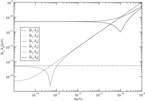
FIG. 2.: The difference $|\lambda_{a}-\lambda_{b}|$ $(a,b=1,2,3,4,~{}a\neq b)$ as a function of the matter density $A$ for a (3+1)-scheme, where $\theta_{12}=\frac{\pi}{4}$, $\theta_{23}=\frac{\pi}{4}$, $\theta_{13}=0$, $\theta_{14}=\epsilon$, $\theta_{24}=\delta=0$, $\theta_{34}=0$, $\Delta m_{21}^{2}\simeq 10^{-4}\mathrm{eV^{2}}$, $\Delta m_{32}^{2}\simeq 10^{-3}\mathrm{eV^{2}}$, $\Delta m_{41}^{2}\simeq 1\mathrm{eV^{2}}$, $E=10$ GeV and $\epsilon=0.1$.

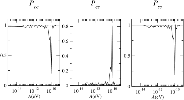
FIG. 3.: The transition probabilities $P_{ee}$, $P_{es}$ and $P_{ss}$ as a function of the matter density $A$ for a (3+1)-scheme, where $\theta_{12}=\frac{\pi}{4}$, $\theta_{23}=\frac{\pi}{4}$, $\theta_{13}=0$, $\theta_{14}=\epsilon$, $\theta_{24}=\delta=0$, $\theta_{34}=0$, $\Delta m_{21}^{2}\simeq 10^{-4}\mathrm{eV^{2}}$, $\Delta m_{32}^{2}\simeq 10^{-3}\mathrm{eV^{2}}$, $\Delta m_{41}^{2}\simeq 1\mathrm{eV^{2}}$, $E=10$ GeV and $L/E=6.46\times 10^{3}\mathrm{eV^{-2}}$. The solid and broken lines show the transition probabilities for $\epsilon=0.1,0$, respectively.

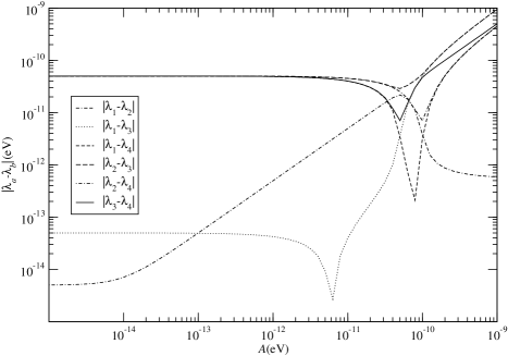
FIG. 4.: The differences $|\lambda_{a}-\lambda_{b}|\quad(a,b=1,2,3,4)$ as a function of the matter density $A$ for a (2+2)-scheme, where $\theta_{14}=\frac{\pi}{4}$, $\theta_{23}=\frac{\pi}{4}$, $\theta_{12}=\epsilon$, $\theta_{13}=0$, $\theta_{24}=0$, $\theta_{34}=0$, $\Delta m_{21}^{2}\simeq 1\mathrm{eV^{2}}$, $\Delta m_{32}^{2}\simeq 10^{-3}\mathrm{eV^{2}}$, $\Delta m_{41}^{2}\simeq 10^{-4}\mathrm{eV^{2}}$, $E=10$ GeV and $\epsilon=0.1$.

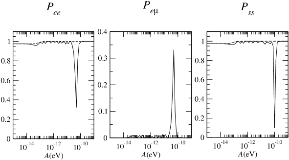
FIG. 5.: The transition probabilities $P_{ee}$, $P_{e\mu}$ and $P_{ss}$ as a function of the matter density $A$ for a (2+2)-scheme, where $\theta_{14}=\frac{\pi}{4}$, $\theta_{23}=\frac{\pi}{4}$, $\theta_{12}=\epsilon$, $\theta_{13}=0$, $\theta_{24}=0$, $\theta_{34}=0$, $\Delta m_{21}^{2}\simeq 1\mathrm{eV^{2}}$, $\Delta m_{32}^{2}\simeq 10^{-3}\mathrm{eV^{2}}$, $\Delta m_{41}^{2}\simeq 10^{-4}\mathrm{eV^{2}}$, $E=10$ GeV and $L/E=6.46\times 10^{3}\mathrm{eV^{-2}}$. The solid and broken lines show the transition probabilities for $\epsilon=0.1,0$, respectively.

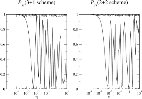
FIG. 6.: The surviving probabilities $P_{ss}$ of the sterile neutrino transition as a function of the rate $\eta$ for a (3+1)-scheme and a (2+2)-scheme, where $L/E=\eta\times 6.46\times 10^{3}{\mathrm{eV^{-2}}}$. We compare $P_{ss}$ at two kinds of the matter densities for $A=1.40\times 10^{-13}$[eV](the broken line) and $A=10^{-10}$[eV](the solid line).

REFERENCES

- [1] Q. R. Ahmad et al., Phys. Rev. Lett. 87, 071301 (2001).
- [2] B. T. Cleveland et al., Astrophys. J. 496, 505 (1998).
- [3] W. Hampel et al., Phys. Lett. B 447, 127 (1999).
- [4] Y. Fukuda et al., Phys. Rev. Lett. 77, 1683 (1996).
- [5] Y. Fukuda et al., Phys. Rev. Lett. 82, 1810 (1999).
- [6] K. Scholberg, for the Super-Kamiokande Collaboration, presented at 8th International Workshop on Neutrino Telescopes, Venice, 1999, e-print hep-ex/9905016.
- [7] J. N. Abdurashitov et al., Phys. Rev. C 60, 055801 (1999).
- [8] C. Athanassopoulos et al., Phys. Rev. Lett. 77, 3082 (1996).
- [9] S. P. Mikheyev and A. Y. Smirnov, Yad. Fiz. 42, 1441 (1985) [Sov. J. Nucl. Phys. 42, 913 (1985)]; S. P. Mikheyev and A. Y. Smirnov, Nuovo Cimento C 9, 17 (1986); L. Wolfenstein, Phys. Rev. D 17, 2369 (1978); L. Wolfenstein, ibid. 20, 2634 (1979).
- [10] S. M. Bilenky, C. Giunti and W. Grimus, Prog. Part. Nucl. Phys. 43, 1 (1999).
- [11] Z. Maki, M. Nakagawa and S. Sakata, Prog. Theor. Phys. 28, 870 (1962).
- [12] T. Ohlsson, H. Snellman, J. Math. Phys. 41, 2768 (2000), ibid. 42, 2345 (2001).
- [13] V. Barger, Y. B. Dai, K. Whisnant and B. L. Young, Phys. Rev. D 59, 113010 (1999).
- [14] V. Barger, B. Kayser, J. Learned, T. Weiler and K. Whisnant, Phys. Lett. B 489, 345 (2000).
- [15] Mathematical Handbook of Formulas and Tables, edited by M. R. Spiegel (McGraw-Hill, Inc., New York, 1968).
- [16] Particle Data Group, C. Caso et al., Review of Particle Physics, Eur. Phys. J. C 3, 1 (1998).
- [17] J. N. Bahcall, Neutrino Astrophysics, (Cambridge Univ. Press, New York, 1989) p. 101.