Towards a New Global QCD Analysis:
  Low $x$ DIS Data from Non-Linear Evolution

Abstract

A new approach to global QCD analysis is developed. The main ingredients are two QCD-based evolution equations. The first one is the Balitsky-Kovchegov nonlinear equation, which sums higher twists while preserving unitarity. The second equation is linear and it is responsible for the correct short distance behavior of the theory, namely it includes the DGLAP kernel. Our approach allows extrapolation of the parton distributions to very high energies available at the LHC as well as very low photon virtualities, $Q^{2}\ll 1\,{\rm GeV^{2}}$.

All existing low $x$ data on the $F_{2}$ structure function is reproduced using one fitting parameter. The resulting $\chi^{2}/df=1$.

Analyzing the parameter $\lambda\equiv\partial\ln F_{2}/\partial(\ln 1/x)$ at very low $x$ and $Q^{2}$ well below $1\,{\rm GeV^{2}}$ we find $\lambda\simeq 0.08-0.1$. A result which agrees with the ”soft pomeron” intercept without involving soft physics.

1 Introduction

In the paper [1] a new approach to DIS was proposed. In the present paper we review and further develop the ideas introduced in Ref. [1]. Our main result is that all existing low $x$ data on the $F_{2}$ structure function can be described by nonlinear QCD evolution.

The standard perturbative QCD approach to deep inelastic scattering (DIS) is based on the DGLAP evolution equation [2] which provides the leading twist parton distributions. The main underlying assumption is that the high twist contributions are negligibly small if the evolution starts at sufficiently high photon virtualities $Q_{0}^{2}\approx 2-4\,(\rm GeV^{2})$.

The approach based on the DGALP equation suffers from three principal problems.

• The DGLAP evolution predicts a steep growth of parton distributions in the region of low $x$ which would eventually contradict the unitarity constraints [3]. Hence, we can expect large unitarity corrections to the DGLAP evolution equation, in the region of very low $x$.

• The second problem is the general nature for any operator product expansion which is an asymptotic series. In application to DIS this means that the errors associated with the leading twist approximation are not small. They are of the order of the next to leading order twist contribution which grows very fast at low $x$. In fact, it can be shown that high twist contributions grow with decreasing $x$ faster than the leading twist [4]. Hence, we cannot conclude that the higher twist contributions are small in the whole kinematic region, even if they are small for the initial value of $Q^{2}=Q^{2}_{0}$. The estimates of Ref. [5] show that all available parameterizations of the solutions to the DGLAP evolution equation lead to substantial higher twist contributions.

• The last problem is in the total nonability of the DGLAP equation to describe physics of low photon virtuality $Q^{2}\leq 1\,(\rm GeV^{2})$. For these kinematics one needs to use Regge phenomenology or other phenomenological models.

It is important to add that NLO DGLAP, though it improves the fits to presently available data, does not solve any of the above principal difficulties. Consequently, we are lead to the conclusion that DGLAP is insufficient to describe all kinematical phase space. For small values of $x$ and/or $Q^{2}$ there is need for a new QCD-based idea.

In this paper, we develop such an idea which allows us to extrapolate parton distributions to very low $x$ (high energies). An extrapolation of the available parton distribution to the region of lower $x$ is a practical problem for the LHC energies. We need to know the parton distribution both for estimates of the background of all interesting processes at the LHC, such as Higgs production, and for the calculation of the cross sections of the rare processes which are likely to be measured at the LHC.

Our method was originally proposed in Ref. [1]. It consists of two steps. As a first step, a nonlinear evolution equation, which takes into account the most significant higher twist contributions, is solved. This equation (2.1) specifies a high energy (low $x$) behavior of the parton densities. The solution obtained, below denoted as $\tilde{N}$, takes into account collective phenomena of high parton density QCD and respects unitarity constraints. Moreover, $\tilde{N}$ can be found for large transverse distances, and so it also provides a possibility to describe data of low photon virtuality.

The parton distributions which we obtain are then amended by adding to the solution of the nonlinear equation $\tilde{N}$, a correcting function $\Delta N$, which is aimed at correctly incorporating the short distance behavior of the theory, namely the DGLAP kernel.

For $\Delta N$ we propose a linear DGLAP-type evolution equation. The function $\Delta N$ is considered to be a small correction to $\tilde{N}$ concentrated in the region of moderate $x$. Consequently, this function should be free of all difficulties inherent in the usual solutions of the DGLAP equation.

The philosophy of our approach is quite similar to the one recently presented by Ref. [6]. That paper is a development of the Golec-Biernat - Wusthoff (GBW) model which in addition to the original model [7] is improved by DGLAP evolution. We can trace a certain analogy between our function $\tilde{N}$ and the original saturation model. Both functions play the very same role: they take into account the gluon saturation effects in unitarity preserving way, and describe physics of large distances. However, contrary to the saturation model the function $\tilde{N}$ is derived from QCD. The DGLAP improvement both in our approach and in Ref. [6] is aimed at correctly incorporating the short distance dynamics however, the technical realizations are quite different.

The paper is organized as follows. In the next section we review our approach and write the BK nonlinear equation for $\tilde{N}$ and a linear equation for $\Delta N$. Section 3 presents some analytical estimates of the corrections induced by the DGLAP kernel. Section 4 is devoted to technical details of numerical solutions of the equations. The following Section (5) presents our fit to the experimental data on $F_{2}$ structure function and its logarithmic derivatives. Some predictions for THERA and LHC are given. Section 6 presents a general discussion which emphasizes some weak points of our approach. In the concluding Section (7) we summarize our results and mention our plans for future work.

2 Reviewing a new approach to DIS

The DGLAP equation describes the gluon radiation which leads to a strong increase in the number of partons. However, when the parton density becomes large, annihilation processes become important and they suppress the gluon radiation taming the rapid growth of the parton density [3, 8, 9]. A development of new theoretical methods applicable to physics of high density QCD [3, 8, 9, 10, 11, 12, 13, 14] lead finally to the very same nonlinear evolution equation, nowadays credited to Balitsky and Kovchegov (BK):

$$\tilde{N}({\mathbf{x_{01}}},Y;b) \,=\, \tilde{N}({\mathbf{x_{01}}},Y_{0};b)\,{\rm exp}\left[-\frac{2\,C_{F}\,\alpha_{S}}{\pi}\,\ln\left(\frac{{\mathbf{x^{2}_{01}}}}{\rho^{2}}\right)(Y-Y_{0})\right]\,+$$ (2.1)

$$\frac{C_{F}\,\alpha_{S}}{\pi^{2}}\,\int_{Y_{0}}^{Y}dy\,{\rm exp}\left[-\frac{2\,C_{F}\,\alpha_{S}}{\pi}\,\ln\left(\frac{{\mathbf{x^{2}_{01}}}}{\rho^{2}}\right)(Y-y)\right]\,\times$$

$$\int_{\rho}\, d^{2}{\mathbf{x_{2}}} \frac{{\mathbf{x^{2}_{01}}}}{{\mathbf{x^{2}_{02}}}\,{\mathbf{x^{2}_{12}}}}\left(\,2\,\tilde{N}({\mathbf{x_{02}}},y;{\mathbf{b-\frac{1}{2}x_{12}}})-\tilde{N}({\mathbf{x_{02}}},y;{\mathbf{b-\frac{1}{2}x_{12}}})\tilde{N}({\mathbf{x_{12}}},y;{\mathbf{b-\frac{1}{2}x_{02}}})\right)$$

The equation is derived for $\tilde{N}(r_{\perp},x;b)$ which stands for imaginary part of the amplitude of a dipole of size $r_{\perp}$ elastically scattered at the impact parameter $b$.

In the equation (2.1), the rapidity $Y=-\ln x$ and $Y_{0}=-\ln x_{0}$. The ultraviolet cutoff $\rho$ is needed to regularize the integral, but it does not appear in physical quantities. In the large $N_{c}$ limit (number of colors) $C_{F}=N_{c}/2$ (we set $N_{c}=3$ in the numerical computations).

Eq. (2.1) has a very simple meaning: the dipole of size $\mathbf{x_{10}}$ decays in two dipoles of sizes $\mathbf{x_{12}}$ and $\mathbf{x_{02}}$ with the decay probability given by the wave function $|\Psi|^{2}\,=\,\frac{\mathbf{x^{2}_{01}}}{\mathbf{x^{2}_{02}}\,\mathbf{x^{2}_{12}}}$. These two dipoles then interact with the target. The non-linear term takes into account a simultaneous interaction of two produced dipoles with the target or, in other words, the Glauber corrections for dipole-target interaction.

The linear part of Eq. (2.1) is the LO BFKL equation [17], which describes the evolution of the multiplicity of the fixed size color dipoles with respect to the energy $Y$. The nonlinear term corresponds to a dipole splitting into two dipoles and it sums the high twist contributions. Note, that the linear part of Eq. (2.1) (the BFKL equation) also has higher twist contributions and vice versa, the main contribution of the non-linear part is to the leading twist (see Ref. [8] for general arguments and Ref. [5] for explicit calculations).

As has been mentioned, the master equation (2.1) is derived in the leading $\ln(1/x)$ approximation of perturbative QCD. This means we consider $\alpha_{S}\ln(1/x)\approx 1$ while $\alpha_{S}\ll 1$ as well as $\alpha_{S}\ln Q^{2}\ll 1$. In other words, the equation sums all contributions of the order $(\alpha_{S}\ln(1/x))^{n}$ and neglects contributions of the orders $\alpha_{S}(\alpha_{S}\ln(1/x))^{n}$ and $\alpha_{S}\ln Q^{2}(\alpha_{S}\ln(1/x))^{n}$. Contributions of the latter will be taken into account by the function $\Delta N$ to be discussed below.

Eq. (2.1) sums all diagrams of the order

$$\left(\,\alpha_{S}^{2}(1/x)^{\Delta}\,\right)^{n}\,\,\mbox{with}\,\,\,\,\Delta\,\,\propto\,\,\alpha_{S}\,.$$

This means that starting from $\alpha_{S}\ln(1/x)\,\,\approx\,\,\ln(1/\alpha_{S})$ corrections due to rescattering and recombination of parton become essential (see Ref. [18] for details).

The next to leading corrections to the DGLAP or/and BFKL equations lead to $\Delta=C_{1}\alpha_{S}+C_{2}\alpha_{S}^{2}$ which start to be important only for $\alpha_{S}\ln(1/x)\geq\,1/\alpha_{S}$. Therefore, the correct strategy is first to solve the master equation taking into account all corrections of the leading order, and only as a second step consider the next-to-leading order corrections.

It is well known starting with Bartel’s paper in Ref. [4] that Eq. (2.1) can be proven in the large $N_{c}$ limit of QCD. Actually, this equation is a first theoretical realization of the Veniziano topological expansion [19]. For $N_{c}\,\,\gg\,\,1$, we assume that $\bar{\alpha}_{s}=N_{c}\alpha_{S}/\pi\approx 1$ while $\alpha_{S}\ll 1$. An interesting feature of the equation is that it depends on $\bar{\alpha}_{S}$ only, and all problems with the accuracy of the large $N_{c}$ expansion are really concentrated in the $N_{c}$ dependence of the initial distributions (see Ref. [18] for details).

It should be stressed that a correct evolution equation without an additional assumption on large $N_{c}$ is known (see Weigert’s paper in Ref. [11]). However, this equation is so complicated that we are far away from its solution. However, it is worthwhile mentioning that in the simplified case of double log approach (both $\alpha_{S}\ln(1/x)$ and $\alpha_{S}\ln Q^{2}$ are of the order unity while $\alpha_{S}\,\ll\,1$) the equation for $N_{c}\approx 1$ was written and solved in Ref. [20]. This solution shows that corrections to large $N_{c}$ approximation are rather small and, therefore, at the first stage it is reasonable to neglect them.

In order to safely use Eq. (2.1) we neede to estimate the neglected contributions. A first class of such contributions is the interaction between two parton showers which leads to $(\bar{\alpha}_{S}/N^{2}_{c})\ln(1/x)$ corrections which result in a bound on minimal $x$:

$$\ln(1/x)\,\,\leq\,\,\frac{N^{2}_{c}}{\bar{\alpha}_{S}}\,.$$

A second constraint comes from so called enhanced diagrams. It turns out that they lead to the very same restrictions as the previous one (see Ref. [18] for details).

The above energy limit is not very essential since the unitarity bound $\tilde{N}=1$ is reached at higher values of $x$. Thus the $1/N_{c}$ corrections cannot modify this result, but could slightly modify the value of the saturation scale.

The total dipole cross section is given by the integration over the impact parameter:

$$\sigma_{\rm dipole}(r_{\perp},x)\,\,=\,\,2\,\,\int\,d^{2}b\,\,\tilde{N}(r_{\perp},x;b).$$ (2.2)

The contribution to the deep inelastic structure function $F_{2}$ which is due to $\tilde{N}$ we denote by $\tilde{F}_{2}$ and it is related to the dipole cross section

$$\tilde{F}_{2}(x,Q^{2})\,\,\,=\,\,\frac{Q^{2}}{4\pi^{2}}\,\int\,\,d^{2}r_{\perp}\int\,dz\,\,P^{\gamma^{*}}(Q^{2};r_{\perp},z)\,\,\sigma_{\rm dipole}(r_{\perp},x)\,\,.$$ (2.3)

The physical interpretation of Eq. (2.3) is transparent. It describes the two stages of DIS [21]. The first stage is the decay of a virtual photon into a colorless dipole ($q\bar{q}$ -pair). The probability of this decays is given by $P^{\gamma^{*}}$. The second stage is the interaction of the dipole with the target ($\sigma_{\rm dipole}$ in Eq. (2.3)). This equation is a simple manifestation of the fact that color dipoles are the correct degrees of freedom in QCD at high energies [15]. The QED wave functions of the virtual photon are well known [15, 22, 23] (we consider only massless case):

$$P^{\gamma^{*}}(Q^{2};r_{\perp},z)^{2}\,=\,\frac{N_{c}}{2\,\pi^{2}}\sum_{f}\,Z_{f}^{2}\,\left\{(z^{2}+(1-z)^{2})\,a^{2}\,K_{1}^{2}(a\,r_{\perp})\,\,+\,\,4\,Q^{2}\,z^{2}\,(1-z)^{2}\,K_{0}^{2}(a\,r_{\perp})\right\}\,,$$ (2.4)

with $a^{2}=Q^{2}z(1-z)$.

It can be seen that Eq. (2.1) does not depend explicitly on the target. All the dependence on the target comes from the initial condition specified at some initial value $x_{0}$. For a target nucleus it was argued in Ref. [13] that the initial conditions should be taken in the Glauber form:

$$\tilde{N}(\mathbf{x_{01}},x_{0};b)\,=\,N_{GM}(\mathbf{x_{01}},x_{0};b)\,,$$ (2.5)

with

$$N_{GM}(\mathbf{x_{01}},x;b)\,=\,1\,\,-\,{\rm exp}\left[-\frac{\alpha_{S}\pi\mathbf{x^{2}_{01}}}{2\,N_{c}\,R^{2}}\,xG^{DGLAP}(x,4/\mathbf{x_{01}^{2}})\,S(\mathbf{b})\right]\,.$$ (2.6)

The equation (2.6) represents the Glauber-Mueller (GM) formula which accounts for the multiple dipole-target interaction in the eikonal approximation [22, 24, 25]. The function $S(b)$ is a dipole profile function inside the target. The value of $x_{0}$ is chosen within the interval

$${\rm exp}(-\frac{1}{\alpha_{S}})\,\leq\,x_{0}\,\leq\frac{1}{2mR}\,\,,$$ (2.7)

where $R$ is the radius of the target. In this region the value of $x_{0}$ is small enough to use the low $x$ approximation, but the production of the gluons (color dipoles) is still suppressed as $\alpha_{S}\ln(1/x)\,\leq\,\,1$. Consequently, in this region we have the instantaneous exchange of the classical gluon fields. Hence, an incoming color dipole interacts separately with each nucleon in a nucleus (see Mueller and Kovchegov paper in Ref. [10]).

For the hadron, however, there is no proof that Eq. (2.5) is correct. Our criteria in this problem (at the moment) is the correct description of the experimental data. Almost all available HERA data can be described using Eq. (2.5) [26, 27], and we feel confident setting Eq. (2.5) as an initial condition for Eq. (2.1). In our model, the Gaussian ($S(b)=e^{-b^{2}/R^{2}}$) form for the profile function of the hadron is mostly used. The parameter $R$ is a phenomenological input, while the gluon density $xG^{DGLAP}$ is a solution of the DGLAP equation. For a hadron target Eq. (2.7) is still correct, but practically $x_{0}=10^{-2}$ is chosen. This value satisfies Eq. (2.7) for which much experimental data exist, so one can check the initial conditions.

Solutions to the BK equation were studied in asymptotic limits in Ref. [28] while several numerical solutions were reported in Refs. [16, 1, 29, 30, 31]. In Ref. [1] and in present paper we solve Eq. (2.1) in the coordinate representation in which the initial conditions are of a very simple form (see Eq. (2.5)). The second reason for using the coordinate representation is the fact that all physical observables can be expressed in terms of the amplitude for the dipole-target interaction in the coordinate representation. Finally, it is also very useful that the long distance asymptotics is known: $\tilde{N}\,\,\rightarrow\,\,1$ being $\tilde{N}\,\,\leq\,\,1$ otherwise. This fact provides a natural control for the numerical procedure.

Unfortunately, Eq. (2.1) is an approximation. It only sums large $\ln x$ contributions. The situation can be improved at short distances. The exact $x$ dependence of the kernel at short distances is known, namely it is the DGLAP kernel. An attempt to obtain the elastic amplitude $\tilde{N}$ based on elements of both the BK and DGLAP equations was presented in Ref. [32]. The authors of this paper first solve a generalized DGLAP-BFKL linear equation [33], and then add to the solution a nonlinear perturbation of the form presented in Eq. (2.1). This approach actually incorporates the high twist contributions in the standard way, treating them as corrections to the leading one.

We suggest a different approach to the problem. First, all twist contributions should be summed by solving Eq. (2.1). Unfortunately, it is complicated to find a solution for an arbitrary value of the impact parameter $b$. We simplify the problem by solving Eq. (2.1) without including the $b$-dependence, this corresponds to case of solving for the initial condition at $b=0$. At the very end we restore the $b$-dependence by using an ansatz to be discussed in Section 4. We denote by $\tilde{N}(r_{\perp},x)$ the solution of Eq. (2.1) at $b=0$.

Secondly, we add to the solution obtained a correcting function $\Delta N$, which will account for the DGLAP kernel (Fig. 1):

$$N\,=\,\tilde{N}\,+\,\Delta N\,\,\,\,\,\,\,\,\,\,\ \,\,for\,\,\,x\,\leq\,x_{0}\,.$$ (2.8)

Figure 1: The kinematic map for the solutions.

In order to extract the leading $\ln\,(1/r_{\perp}^{2})$ contributions we define a set of new functions:

$$\tilde{n}\,\equiv\,\tilde{N}/(\alpha_{s}\,r_{\perp}^{2})\,;\,\,\,\,\,\,\,\,\,\,\,n\,\equiv\,N/(\alpha_{s}\,r_{\perp}^{2})\,;\,\,\,\,\,\,\,\,\,\,\,\,\Delta n\,\equiv\,\Delta N/(\alpha_{s}\,r_{\perp}^{2})\,.$$

For the function $n$ we propose the following nonlinear equation assumed to be valid in the leading large $\ln\,(1/r_{\perp}^{2})$ approximation:

$$\frac{\partial n(r_{\perp},x)}{\partial\,\ln(1/r_{\perp}^{2})}\,=\,\frac{C_{F}\,\alpha_{s}}{\pi}\int_{x}^{1}\,P_{g\rightarrow g}(z)\,\,n(r_{\perp},\frac{x}{z})\,dz\,\,-\,\,\frac{C_{F}\,\alpha_{s}^{2}\,r^{2}_{\perp}}{\pi}\int_{x/x_{0}}^{1}\frac{dz}{z}\,n^{2}(r_{\perp},\frac{x}{z})\,.$$ (2.9)

Here $P_{g\rightarrow g}(z)$ stands for the usual gluon splitting function:

$$P_{g\rightarrow g}(z)\,=\,2\,\left[\frac{1-z}{z}\,+\,\frac{z}{(1-z)_{+}}\,+\,z\,(1-z)\,+\,\left(\frac{11}{12}-\frac{n_{f}}{18}\right)\delta(1-z)\right]\,.$$ (2.10)

Note that we assume nonlinear effects to be of no importance for $x>x_{0}$. Eq. (2.1) can be rewritten in the large $\ln(1/r_{\perp}^{2})$ approximation as:

$$\frac{\partial\tilde{n}(r_{\perp},x)}{\partial\,\ln(1/r_{\perp}^{2})}\,=\,\frac{\partial\tilde{n}(r_{\perp},x_{0})}{\partial\,\ln(1/r_{\perp}^{2})}\,+\,\,\frac{C_{F}\,\alpha_{s}}{\pi}\int_{x}^{1}\,\frac{dz}{z}\,\,\tilde{n}(r_{\perp},\frac{x}{z})\,\,-\,\,\frac{C_{F}\,\alpha_{s}^{2}\,r^{2}_{\perp}}{\pi}\int_{x/x_{0}}^{1}\frac{dz}{z}\,\tilde{n}^{2}(r_{\perp},\frac{x}{z})\,.$$ (2.11)

Subtracting Eq. (2.11) from Eq. (2.9) and assuming $\Delta N$ to be small compared to $\tilde{N}$, we derive the equation for $\Delta n(r_{\perp},x)$:

$$\frac{\partial\Delta n(r_{\perp},x)}{\partial\,\ln(1/r_{\perp}^{2})}\,=\,\frac{C_{F}\alpha_{S}}{\pi}\int_{x/x_{0}}^{1}\,P_{g\rightarrow g}(z)\,\,\Delta n(r_{\perp},\frac{x}{z})\,dz-$$ (2.12)

$$\frac{2\,C_{F}\,\alpha_{s}}{\pi}\int_{x/x_{0}}^{1}\frac{dz}{z}\,\tilde{N}(r_{\perp},\frac{x}{z})\Delta n(r_{\perp},\frac{x}{z})+\frac{C_{F}\,\alpha_{s}}{\pi}\,\int_{x/x_{0}}^{1}\left(P_{g\rightarrow g}(z)-\frac{2}{z}\right)\tilde{n}(r_{\perp},\frac{x}{z})\,dz$$

$$-\frac{\partial\tilde{n}(r_{\perp},x_{0})}{\partial\,\ln(1/r_{\perp}^{2})}\,\,+\,\,\frac{C_{F}\,\alpha_{s}}{\pi}\int_{x}^{x/x_{0}\,-}\,P_{g\rightarrow g}(z)\,\,n(r_{\perp},\frac{x}{z})\,dz\,.$$

Equation (2.12) is a linear equation valid in the leading $\ln(1/r_{\perp}^{2})$ approximation. The first term on the right hand side of Eq. (2.12) is the DGLAP evolution for the correcting function $\Delta N$, while the second term is the ”nonlinear interaction” of the solutions. The third term in the equation represents the correction which is due to the substitution of the BFKL kernel $1/z$ by the correct DGLAP kernel.

The last term in (2.12) is the only term which accounts for the contribution of high $x>x_{0}$. In that region the function $n=\pi\,xG^{DGLAP}/(2N_{c}R^{2})$ being a solution of the DGLAP equation is not given by a sum of $\tilde{n}$ and $\Delta n$. The sign ”-” in the upper integration limit indicates that in the limit $x\rightarrow x_{0}$ the $\delta$-function term of the splitting function must be excluded.

If we set $\tilde{N}=0$ then Eq. (2.12) reduces exactly to the gluonic part of the leading order DGLAP equation. In planned further development of our approach quark distributions and their evolution will also be included. At the present stage we take them into account implicitly in $\alpha_{s}$ and by setting $n_{f}=3$ in $P_{g\rightarrow g}$.

The last two terms in Eq. (2.12) were omitted in Ref. [1] as they are not important at low $x$. However they should be included for correct computations.

The initial condition $\Delta N(r_{\perp 0},x)=N(r_{\perp 0},x)-\tilde{N}(r_{\perp 0},x)$ is a phenomenological input at some initial transverse distance $r_{\perp 0}$ to be specified. However, our strategy is based on the assumption that $\tilde{N}$ describes the long distance physics correctly. Consequently, in order to eliminate any discontinuity of the function $N$ we require

$$\Delta N(r_{\perp\,0},x)=0\,.$$ (2.13)

The value of $r_{\perp\,0}$ is not specified but it is expected to be of the order $2\,(\rm GeV^{-1})$ corresponding to the naive relation $Q_{0}^{2}=4/r^{2}_{\perp\,0}\simeq 1\,(\rm GeV^{2})$.

Since we assume $\tilde{N}(r_{\perp},x_{0})$ to describe correctly the data at $x=x_{0}$, the continuity across $x=x_{0}$ supposes that $\tilde{N}(r_{\perp},x_{0})\,=\,N(r_{\perp},x_{0})$. If we require this equality then Eq. (2.12) would respect it provided initial condition (2.13) is imposed.

It is important to emphasize that Eq. (2.12) is free from the main problems of the DGLAP equation. First of all, the high twist contributions are summed (at least partially) by Eq. (2.1). Secondly, our method respects unitarity. This is achieved due to the second term of Eq. (2.12) and the unitarity preserving initial condition (2.13).

Finally it is necessary to compute a correction to $F_{2}$ structure function due to $\Delta N$. To achieve this goal we need to assign an impact parameter dependence of $\Delta N$. Similarly to what is common in DGLAP solutions, the $b$-dependence is assumed to be a product of $(2\,\pi\,R^{2})\Delta N$ times a profile function. After $b$-integration the latter contributes unity. Then the correction to $F_{2}$ reads

$$\Delta F_{2}(x,Q^{2})\,=\,\frac{4\,N_{c}}{9\,\pi^{3}}\,\int_{4/Q^{2}}^{r_{\perp\,0}}\,\frac{dr_{\perp}^{2}}{r_{\perp}^{4}}\,\,\Delta N(r_{\perp},x)\,(\pi\,R^{2})\,.$$ (2.14)

The $r_{\perp}$ integration in (2.14) is evaluated in the same large $\ln 1/r_{\perp}$ approximation as is valid for Eq. (2.12). Note that the coefficient $(\pi\,R^{2})$ is cancelled with the same factor hidden in $\Delta N$.

3 DGLAP correction - analytical estimates

In this section we would like to make some comments regarding the consistency of our approach. It was argued previously that it is necessary to add a correction term $\Delta N$ to the solution $\tilde{N}$ of the nonlinear equation (2.1), where the function $\Delta N$ is a solution of the evolution equation (2.12).

Consistency of the approach requires the function $\Delta N$ to give vanishing contributions to the dipole cross section at very small $x$. We also expect this function to decrease as $r_{\perp}^{2}$ decreases. Finally, $\Delta N$ is assumed to be a small correction to the function $\tilde{N}$. In order to check the above conditions some asymptotic estimates can be made without explicitly solving Eq. (2.12). Indeed, we will show below that Eq. (2.12) respects all the above mentioned requirements.

• Limit 1: fixed $r_{\perp}$, $x\rightarrow 0$.

  At very small $x$ and fixed distances the function $\tilde{N}\simeq 1$. Eq. (2.12) can be simplified:

  $$\frac{\partial\Delta n(r_{\perp},x)}{\partial\ln(1/r_{\perp}^{2})}\,=\,\frac{C_{F}\alpha_{S}}{\pi}\int_{x/x_{0}}^{1}\,\left(P_{g\rightarrow g}(z)-\frac{2}{z}\right)\,\left(\tilde{n}(r_{\perp},\frac{x}{z})\,+\,\Delta n(r_{\perp},\frac{x}{z})\right)\,dz\,.$$ (3.15)

  The main observation is that the evolution kernel entering the equation (3.15) is actually negative. Hence the function $\Delta n$ decreases as $r_{\perp}$ decreases.

  Let us consider a model where the anomalous dimension has the form consistent with energy conservation [34]

  $$\gamma(\omega)\,=\,\bar{\alpha}_{S}\left(\frac{1}{\omega}\,-\,1\right)\,,$$ (3.16)

  where $\bar{\alpha}_{S}\equiv\alpha_{S}N_{c}/\pi$ and the anomalous dimension is defined by the Mellin transform of the splitting function $P_{g\rightarrow g}$:

  $$\gamma(\omega)\,=\,\frac{\alpha_{S}\,C_{F}}{\pi}\int_{0}^{1}\,dz\,P_{g\rightarrow g}(z)\,z^{\omega}.$$ (3.17)

  Eq. (3.15) can be solved using the inverse Mellin transform [1]. Define $\Delta n(r_{\perp},\omega)$ and $\tilde{n}(r_{\perp},\omega)$ as the inverse Mellin transforms

  $$\Delta n(r_{\perp},\omega)\,\equiv\,\frac{1}{2\,\pi\,i}\,\int_{C}\,d\omega\,x^{-\omega}\,\Delta n(r_{\perp},\omega)\,;\,\,\,\,\,\,\,\,\,\,\,\,\,\,\,\,\tilde{n}(r_{\perp},\omega)\,\equiv\,\frac{1}{2\,\pi\,i}\,\int_{C}\,d\omega\,x^{-\omega}\,\tilde{n}(r_{\perp},\omega)\,.$$

  In the momentum representation Eq. (3.15) together with the anomalous dimension (3.16) is:

  $$\frac{\partial\Delta n(r_{\perp},\omega)}{\partial\ln(1/r_{\perp}^{2})}\,=\,-\bar{\alpha}_{s}\,[\tilde{n}(r_{\perp},\omega)\,+\,\Delta n(r_{\perp},\omega)]$$ (3.18)

  Eq. (3.18) can be easily integrated. Applying again the approximation $\tilde{N}\simeq 1$ we get the result for the correcting function $\Delta N$:

  $$\Delta N(r_{\perp},x)\,\simeq\,-\frac{\bar{\alpha}_{S}}{1+\bar{\alpha}_{S}}\tilde{N}(r_{\perp},x)\,+\,C(x)\,(r_{\perp}^{2})^{1+\bar{\alpha}_{S}}\,.$$ (3.19)

  The function $C(x)$ should be determine from the initial condition $\Delta N(r_{\perp\,0},x)=0$. Consequently

  $$\Delta N(r_{\perp},x)\,\simeq\,-\frac{\bar{\alpha}_{S}}{1+\bar{\alpha}_{S}}\,\left[\tilde{N}(r_{\perp},x)\,-\,\tilde{N}(r_{\perp\,0},x)\,(r_{\perp}^{2}/r^{2}_{\perp\,0})^{1+\bar{\alpha}_{S}}\right]\,.$$ (3.20)

  As expected the function $\Delta N$ is negative and of the order $O(\alpha_{S})$ compared to $\tilde{N}$. As $r_{\perp}$ decreases, $\Delta N$ decreases until it reaches a minimum at $r_{\perp\,min}$ determined by the equation

  $$\frac{\partial\tilde{N}(r_{\perp},x)}{\partial r_{\perp}^{2}}|_{r_{\perp}=r_{\perp\,min}}\,\simeq\,(1+\bar{\alpha}_{S})\,\tilde{N}(r_{\perp\,0},x)\,\frac{(r_{\perp}^{2})^{\bar{\alpha}_{S}}}{(r_{\perp\,0}^{2})^{1+\bar{\alpha}_{S}}},.$$ (3.21)

  At shorter distances $\Delta N$ tends to $0$ as it should.

  Note that at fixed $r_{\perp}$, $\Delta N$ is finite and non vanishing at $x\rightarrow 0$. Yet, this is consistent with the requirement of a vanishing contribution to the dipole cross section since the latter implies integration over the impact parameter $b$. We will assign different $b$-dependences to the functions $\tilde{N}$ and $\Delta N$. After the integration, the dipole cross section due to $\tilde{N}$ will grow logarithmically with $x$, while the contribution of $\Delta N$ will remain finite.

• Limit 2: fixed $x$, $r_{\perp}\rightarrow 0$.

  We would now like to address a question of the short distance asymptotics. In this limit, the function $\tilde{N}$ is given by the solution of the BFKL equation. Namely,

  $$\tilde{N}(r_{\perp},\omega)\,\sim\,e^{\,\,\bar{\alpha}_{S}\,\ln(1/r_{\perp}^{2})/\omega}\,.$$ (3.22)

  On the other hand, energy conservation (3.16) requires

  $$N(r_{\perp},\omega)\,\sim\,e^{\,\,\bar{\alpha}_{S}\,\ln(1/r_{\perp}^{2})\,(1/\omega-1)}\,.$$

  Hence

  $$\Delta N(r_{\perp},\omega)\,\simeq\,\tilde{N}(r_{\perp},\omega)\,(e^{\,\,-\,\bar{\alpha}_{S}\,\ln(1/r_{\perp}^{2})}\,-\,1)\,\rightarrow\,-\,\tilde{N}(r_{\perp},\omega).$$ (3.23)

Finally we conclude that the function $\Delta N$ is supposed to be negative. We expect $\Delta N\,\simeq\,\beta\,\tilde{N}$ with $|\beta|<1$ and to be approximately $x$ independent. At short distances $\Delta N$ tends to zero as $\tilde{N}$.

Therefore, $\Delta N$ turns out to be small in the whole kinematic region. The analysis presented above justifies the self consistency of our approach and paves the way for numerical calculations to be presented in the next section.

4 Numerical solution of the equations

In this section we report on the exact numerical solution of Eq. (2.1) with initial condition (2.5) and of Eq. (2.12) with initial condition (2.13).

First of all we wish to discuss several technical details.

$\bullet$ Kinematic domain

The kinematic region where the solutions of (2.1) and (2.12) are found, covers $x$ values from $x=x_{0}=10^{-2}$, where the initial conditions are set, to $x=10^{-7}$. The maximal transverse distance $r_{\perp}$ is taken to be two fermi. The value of the ultraviolet cutoff $\rho$ is $2\times 10^{-3}\,({\rm GeV^{-1}})$. The numerical solutions obtained are checked and are independent of this choice.

$\bullet$ Coupling constant $\alpha_{S}$.

Eq. (2.1) is derived for constant $\alpha_{S}$. However, the DGLAP equation and hence Eq. (2.9) have a running coupling constant. Consequently, the derivation of Eq. (2.12) implies the same running $\alpha_{S}$ in Eq. (2.1). For numerical purposes we take the LO running $\alpha_{S}$ with $\alpha_{S}=\alpha_{S}(4/r_{\perp}^{2})$ everywhere. At large distances we freeze $\alpha_{S}$ at the value $\alpha_{S}\simeq 0.5$.

$\bullet$ Transverse hadron size $R^{2}$.

In Ref. [1] the fixed value $R^{2}=10\,({\rm GeV}^{-2})$ was taken. This choice corresponds to the value which is obtained from the “soft” high energy phenomenology [35, 36], and is in agreement with the HERA data on elastic $J/\Psi$ photo-production [37]. As $R^{2}$ is practically the only fitting parameter at our disposal we allow it to vary in order to fit the $F_{2}$ data. The optimal fit is achieved at the value $R^{2}\simeq 3.1\,({\rm GeV}^{-2})$. This value is too small and requires our understanding. The physical meaning of such a small value will be considered in the Discussion.

$\bullet$ Gluon density $xG^{DGLAP}$.

In our approach, the gluon density $xG^{DGLAP}$ appears twice: first, in initial condition (2.5) and, second, it accounts for the region $x>x_{0}$ in Eq. (2.12). At this stage, we do not solve the DGLAP equation for the high $x$ region. Instead, we rely on the existing parton distributions. Practically for $xG^{DGLAP}(x\geq x_{0},4/r^{2}_{\perp})$ we use the LO CTEQ6 parametrization [38].

$\bullet$ Solution of Eq. (2.1).

In Ref. [1] Eq. (2.1) was solved by the method of iterations. In the present work we adopt another method which appears to be more efficient. Namely, we solve Eq. (2.1) as an evolution equation in rapidity with a fixed grid in $r_{\perp}$ space and a dynamical step in $Y$. The results of the new program are in total agreement with the old method of Ref. [1] provided the very same initial input is used. The function $\tilde{N}$ is shown in Fig. 2 (solid curves). At large distances, $\tilde{N}$ saturates to unity, which is the unitarity bound. At short distances, $\tilde{N}$ tends to zero indicating color transparency.

$x=10^{-2}$	$x=10^{-3}$	$x=10^{-5}$	$x=10^{-6}$

Figure 2: The solution of Eq. (2.1) (solid line) and Eq. (2.12) (dashed line) plotted versus $r_{\perp}$.

$\bullet$ Large distances.

It is of crucial importance for our purposes to correctly determine $\tilde{N}$ at large transverse distances. However, initial conditions (2.5) are not computable at large distances. The gluon parametrization appearing in Eq.(2.5) ends at $r_{\perp}\simeq 0.5\,fm$. A resolution of the problem was suggested in Ref. [39]. The function $\tilde{N}$ possesses a property called geometrical scaling. Namely, $\tilde{N}(r_{\perp},x)$ is not a function of two independent variables but rather a function of single variable $\tau=r_{\perp}\,Q_{s}(x)$. Here $Q_{s}(x)$ stands for the saturation momentum scale.

The solution $\tilde{N}$ presented in Fig. 2 is obtained in two steps. First, initial conditions (2.5) are extrapolated to long distances by a constant, which at very long distances does not approach unity (such a procedure is not consistent with scaling that is a purely dynamical property of the evolution equation). Then a solution is obtained for all $x$. At sufficiently low $x$ ($x\leq 10^{-4}$) the initial conditions are forgotten and the dynamics is governed by pure evolution. In this region the geometrical scaling is manifested. As a second step, we take the solution thus obtained at $x\simeq 10^{-6}$ and use geometrical scaling in order to rescale this solution up to $x=x_{0}$. The resulting curve is now used for a new long distance extrapolation of initial condition (2.5). The initial condition obtained this way provides a smooth extrapolation of the Glauber formula to unity at very large distances.

Finally, we note that the procedure presented above can be used for large distance extrapolation of the gluon density at high $x>x_{0}$.

$\bullet$ $b$-dependence of the solution.

We assume that solution of the equation (2.1) preserves the same $b$-dependence as introduced by the initial conditions (2.5):

$$\tilde{N}(r_{\perp},x;b)\,=\,(1\,-\,e^{-\kappa(x,r_{\perp})\,S(b)})\,,$$ (4.24)

where $\kappa$ is related to the $b=0$ solution

$$\kappa(x,r_{\perp})\,=\,-\,\ln(1\,-\,\tilde{N}(r_{\perp},x,b=0)).$$ (4.25)

A factorized form of the $b$-dependence was recently advocated in Ref. [40]. The ansatz is quite good at moderate $x$, though it becomes worse at smaller $x$ [1, 30]. The overall uncertainty of the approximation can be roughly estimated not to exceed 10%-20%.

We now proceed with the evaluation of the dipole cross section Eq. (2.2). Having assumed (4.24), the dipole cross section has the form

$$\sigma_{\rm dipole}\,=\,2\,\pi\,R^{2}\,\left[\ln(\kappa)\,+\,E_{1}(\kappa)+\gamma\right]\,.$$ (4.26)

In equation (4.26) $\gamma$ denotes the Euler constant, while $E_{1}$ is the exponential integral function. The expression (4.26) predicts the $\ln{\kappa}$ growth of the dipole cross section, which is in agreement with the conclusions presented in Ref. [28].

$\bullet$ Continuity at $x=x_{0}$.

In Section 2 we discussed the continuity of the function $N$ at $x=x_{0}$. One of the ways for its realization is to require $\Delta N(r_{\perp},x_{0})=0$ which is fulfilled when $N(r_{\perp},x_{0})=\tilde{N}(r_{\perp},x_{0})$. However, $\tilde{N}(r_{\perp},x_{0})$ is given by GM formula (2.5) plus the large distance extrapolation while $N\sim\alpha_{S}\,r_{\perp}^{2}\,xG^{DGLAP}$. Formally they do not coincide though numerical differences are not significant. Nevertheless, we decided to force the equality $N(r_{\perp},x_{0})=\tilde{N}(r_{\perp},x_{0})$. To achieve this, the following changes were introduced in Eq. (2.12).

$$a)\,\,\,\,\,\,\,\,\,\,\,\,\,\,N\,\,\rightarrow\,\,GM\,;\,\,\,\,\,\,\,\,\,\,\,\,\,\,\,\,\,\,b)\,\,\,\,\,\,\,\,\,\frac{\partial\tilde{n}(r_{\perp},x_{0})}{\partial\ln(1/r_{\perp}^{2})}\,\,\rightarrow\,\,\frac{C_{F}\,\alpha_{S}}{\pi}\,\,\int_{x_{0}}^{1}\,dz\,P_{g\rightarrow g}(z)\,n(r_{\perp},x_{0}/z)\,.$$

The above changes are minor. Practically they affect only the long distance behavior of the theory for $x\geq x_{0}$, which is not significant.

$\bullet$ Solution of Eq. (2.12).

Having obtained the function $\tilde{N}$ we can search for the correction $\Delta N$. Eq. (2.12) is solved similarly to Eq. (2.1), but with a fixed grid in rapidity and dynamical step in $r_{\perp}$. The initial conditions (2.13) are set at $r_{\perp}=r_{\perp\,0}$. The parameter $r_{\perp\,0}$ is an adjusting parameter to be determined from the optimal fit. The dashed curves in Fig. 2 show the correcting function $\Delta N$ corresponding to $r_{\perp\,0}=2\,({\rm GeV^{-1}})$.

The function $\Delta N$ obtained displays all the qualitative properties deduced analytically. As expected, starting from zero at $r_{\perp\,0}$ the function $\Delta N$ decreases until it reaches a minimum and then it increases to zero again at asymptotically short distances. The ratio $|\Delta N|/\tilde{N}$ increases permanently during the evolution reaching about 70% at the edge of our kinematic domain. Below $x\simeq 10^{-3}$ this ratio is almost $x$-independent.

5 Results

5.1 Fitting strategy

Low $x$ $F_{2}$ data is used to determine the parameters of our model. The experimental data for $x\leq 10^{-2}$ is taken from ZEUS [41, 42], H1 [43], and E665 [44] experiments. The overall number of points is about 345. We actually use the very same data as Ref. [6]. Statistical and systematic errors are added in quadrature. Whole data sets are allowed to be shifted within the overall normalization uncertainity. We use this freedom to shift the low $Q^{2}$ ZEUS data down by 2% and E665 data by 3%. The H1 data were shifted up by 3%.

Our fitting procedure is divided in two steps. First, recall that in our approach the function $\tilde{N}$ is supposed to describe correctly the kinematical region of very low $x$ and large $r_{\perp}$. The only fitting parameter for $\tilde{N}$ is $R^{2}$. We vary $R^{2}$ in order to find an optimal fit for the $F_{2}$ subset of data below $Q^{2}\simeq 1\,(\rm GeV^{2})$ (about 100 points). The resulting $\chi^{2}/df=1.2$ is achieved for $R^{2}=3.1\,(GeV^{-2})$.

The function $\tilde{N}$ obtained by fitting low $Q^{2}$ subset of the data, is not capable of describing all data points. The fit to all points leads to $\chi^{2}/df>3$, which is not good. The reason for this mismatch is certainly due to the absence of the DGLAP kernel in the evolution of $\tilde{N}$. In order to solve this problem we switch on the DGLAP correction $\Delta N$ which is our second step on the way to the optimal fit. To achieve this Eq. (2.12) is solved.

For $\Delta N$ the only fitting parameter is the position $r_{\perp\,0}$ at which the initial conditions (2.13) are set. It appears, however, that variation of this position acts as a fine tuning parameter only. The optimal fit is realized at $r_{\perp\,0}=2\,(\rm GeV^{-1})$ in total agreement with the underlying theoretical assumptions.

5.2 Fit to $F_{2}$ data

In this subsection we present results of the fit to the low $x$ $F_{2}$ data. The structure function $F_{2}$ is given by a sum of three contributions:

$$F_{2}\,=\,\tilde{F}_{2}\,+\,\Delta F\,+\,F_{2}^{NSQ}\,,$$ (5.27)

where the first two terms are given by Eqs. (2.3) and (2.14). These terms take into account only the gluon contribution to $F_{2}$. In fact, gluons are related to singlet quark distributions. The third term in (5.27) takes into account contributions of non-singlet quark distributions:

$$F_{2}^{NSQ}\,\,=\,\,\sum_{i=u,d}\,\,e_{i}^{2}\,\,q_{i}^{V}\,.$$ (5.28)

In the present stage of our research we borrow the valence quark distributions ($q_{i}^{V}$) from the LO CTEQ6 parametrization. It is important to note, however, that these distributions decrease with decreasing $x$ and are of practically no significance below $x\simeq 10^{-3}$. In future we plan to develop a fully self consistent approach without relying on any known parametrization.

Our central results are presented in Fig. 3 for small $Q^{2}$ (a) and for large $Q^{2}$ (b). The solid line is the best fit obtained with resulting $\chi^{2}/df=1$. The dashed line is a result obtained without the DGLAP correction $\Delta N$ ($\chi^{2}/df>3$).

(a)	(b)

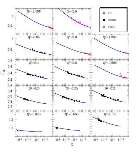
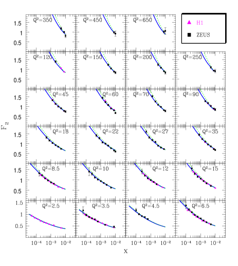
Figure 3: Fit to the $F_{2}$ structure function.

The quality of our fit is of the same level as of Ref. [6]. A similar quality fit was also obtained on a basis of a new scaling saturation model of Ref. [45].

5.3 $dF_{2}/d(\ln Q^{2})$

The logarithmic derivative of $F_{2}$ with respect to $\ln Q^{2}$ is presented in Fig. 4 at fixed $Q^{2}$ (a) and at fixed $x$ (b). Only comparison with H1 data [43] is shown though similar ZEUS measurement exists as well [46]. Note that these experimental data were not take into account in the fitting procedure.

(a)	(b)

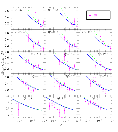
Figure 4: The logarithmic derivative $\partial F_{2}/\partial\ln Q^{2}$.

5.4 $d\ln F_{2}/d(\ln 1/x)$

In this subsection we present our computation of $\lambda\equiv\partial\ln F_{2}/\partial(\ln 1/x)$. A comparison with the H1 data [47] is shown in Fig. 5 at fixed $Q^{2}$ (a) and at fixed $x$ (b).

(a)	(b)

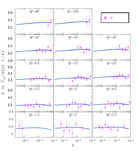
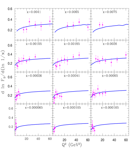
Figure 5: The logarithmic derivative $\lambda\,=\,\partial\ln F_{2}/\partial\ln 1/x$.

Fig. 6 presents our prediction for $\lambda$ at very low $x$ and small values of $Q^{2}$. At fixed $Q^{2}$, $\lambda$ decreases with decreasing $x$ tending to zero in agreement with the unitarity constrain. At $Q^{2}$ well below $1\,GeV^{2}$ and $x\simeq 10^{-6}$, $\lambda\simeq 0.08\pm 0.01$. This value of $\lambda$ coincides with the ”soft pomeron” intercept of the Donnachie and Landshoff model (DL) [35]. It is important to stress that the result is obtained on a basis of perturbative QCD. The only nonperturbative input in our approach is the freezing of $\alpha_{S}$ at large distances. In fact, it was conjectured in Ref. [48] that the soft pomeron may appear in perturbative QCD due to freezing of $\alpha_{S}$.

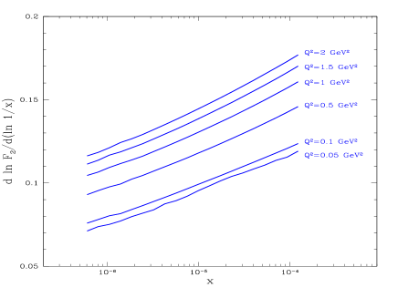
Figure 6: The logarithmic derivative $\lambda\,=\,\partial\ln F_{2}/\partial\ln 1/x$ plotted at low $Q^{2}$ and very low $x$.

5.5 Prediction for $F_{L}$ at HERA

In this subsection we present our prediction for the $F_{L}$ structure function. The result is obtained on a basis of the function $\tilde{N}$ (longitudinal part of $\tilde{F}_{2}$) (Fig. 7). The function $\Delta N$ is obtained within the leading logarithmic approximation, and in this approximation it does not contribute to $F_{L}$. Note that at relatively high values of $x\simeq 10^{-2}\,-\,10^{-3}$ our prediction can be slightly underestimated since the contribution of the valence quarks is neglected.

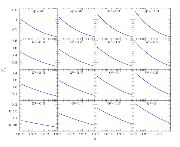
Figure 7: Prediction for the $F_{L}$ structure function at the HERA kinematics. The values of $Q^{2}$ are given in $GeV^{2}$.

5.6 Predictions for LHC and THERA

5.6.1 Gluon density

From the solutions obtained we can compute the gluon density. To this goal we rely on the Mueller‘s formula [22] which relates the density to the elastic dipole-target amplitude:

$$xG(x,Q^{2})\,=\,\frac{4}{\pi^{3}}\,\int_{x}^{1}\,\frac{dx^{\prime}}{x^{\prime}}\,\int_{4/Q^{2}}^{r_{\perp\,0}}\,\frac{dr_{\perp}^{2}}{r_{\perp}^{4}}\,\int\,d^{2}b\,\,2\,\,N(r_{\perp},x^{\prime})\,.$$ (5.29)

Practically we integrate in $x^{\prime}$ up to $x_{0}$ and then add $xG^{DGLAP}(x_{0})$. Fig. 8 presents a comparison between the gluon density obtained from Eq. (5.29) and $xG^{CTEQ}$. At very low $x$ a significant damping of the density can be observed compared to the DGLAP predictions.

Figure 8: The gluon density $xG$ is plotted versus $x$ at fixed $Q^{2}$. The solid line corresponds to Eq. (5.29) while the dashed line is for $xG^{DGLAP}$ (CTEQ6).

5.6.2 $F_{2}$

The obtained model allows extrapolation of the parton distributions to very high energies. Fig. 9 presents our predictions for THERA and LHC kinematics.

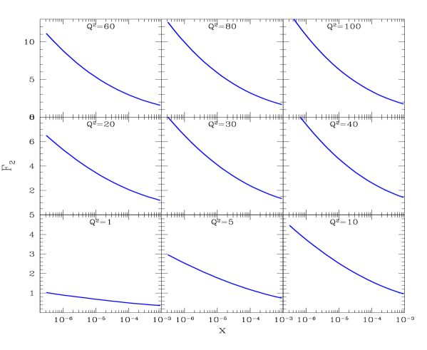
Figure 9: Prediction for the $F_{2}$ structure function at the LHC kinematics. The values of $Q^{2}$ are given in $GeV^{2}$.

6 Discussion

6.1 The transverse hadron size $R^{2}$.

As was pointed out above the optimal fit is achieved for $R^{2}=3.1\,(\rm GeV^{-2})$. Such a low value requires understanding and below we present several explanatory arguments.

1. First of all, the Glauber - Mueller formula of Eq. (2.6) can be used for a proton target with great reservations because contrary to the nuclear case large inelastic diffraction is present. This process not only has a considerable cross section but also a quite different impact parameter dependence corresponding to a small value of the radius. The effect of two different radii is in agreement with the HERA data on elastic and inelastic $J/\Psi$ photo-production [49]. In the simple additive quark model (AQM) there are two kinds of processes: rescattering of a dipole off one quark and rescattering due to interaction with two or even three constituent quarks. The admixture of the inelastic diffractive processes can be taken into account (see Ref. [50] ) by effective decreasing of $R^{2}$ in Eq. (2.6) from 10 $(\rm GeV^{-2})$ to 5 $(\rm GeV^{-2})$.

2. Second, in Eq. (2.6) we used the Gaussian parametrization for $b$-dependence. On the other hand, the data on $J/\Psi$ production requires assuming the profile function of the form [51]:

   $$S(b)=\frac{1}{\pi\,R^{2}}\frac{\sqrt{8}b}{R}K_{1}(\frac{\sqrt{8}b}{R})$$ (6.30)

   which corresponds to the power - like (dipole) form factor in momentum transfer representation:

   $$F_{dipole}(t)=\frac{1}{(1-\frac{1}{8}R^{2}\,t)^{2}}\,.$$ (6.31)

   $F_{dipole}(t)$ describe a system with the same radius $R$ as the Gaussian form factor. In t-representation the latter looks as

   $$F_{exp}(t)=e^{\frac{1}{4}R^{2}\,t}\,\,.$$ (6.32)

   Practically, the solution to the non-linear BK evolution equation is obtained at $b=0$. Note that $S_{dipole}(b=0)=2\,S_{Gaussian}(b=0)$ and this difference can be interpreted as an effective decrease in the value of $R^{2}$. In fact, a relatively good fit to the low $x$ data can be obtained with the dipole profile function at $R^{2}\simeq 4.5\,(\rm GeV^{-2})$.

3. In Eq. (2.6) we use the following expression for the dipole - proton cross section:

   $$\sigma_{dipole}\,=\,\frac{\alpha_{S}\,\pi^{2}\,r^{2}_{\perp}}{N_{c}}xG(x,\frac{4}{r^{2}_{\perp}})\,\,,$$ (6.33)

   However, the expression Eq. (6.33) is an approximation valid for small values of the anomalous dimension $\gamma$ only. The correct expression for the cross section was obtained in Ref. [52]:

   $$\sigma_{dipole}(r_{\perp},x)\,=\,\frac{16\,C_{F}}{N_{c}^{2}-1}\,\pi^{2}\,\int\phi(x,l^{2})\,\,(1-e^{i\,l\,r_{\perp}})\,\frac{\alpha_{S}(l^{2})}{2\pi}\,\frac{d^{2}l}{l^{2}}$$ (6.34)

   with $\phi\equiv\partial xG(x,l^{2})/\partial l^{2}$ being an unintegrated gluon density [17]. The gluon density $xG\equiv xG^{DGLAP}$ is a solution of the DGLAP equation

   $$xG(x,l^{2})\,=\,\frac{1}{2\,\pi\,i}\,\int_{C}d\omega\,x^{-\omega}\,g(\omega)\,e^{\gamma(\omega)\,\ln l^{2}}\,.$$ (6.35)

   Substituting Eq. (6.35) into Eq. (6.34) and performing the $l$-integration we obtain:

   $$\sigma_{dipole}\,=\,\frac{4\,\alpha_{S}\,\pi^{2}}{N_{c}}\,\int_{C}\,\,\frac{d\omega}{2\,\pi\,i}\,\,g(\omega)\,\,e^{\omega\,\ln(1/x)}\,\frac{1}{1-\gamma(\omega)}\,\,\,\left(\,\frac{r^{2}_{\perp}}{4}\right)^{1\,-\,\gamma(\omega)}\,\,\frac{\Gamma(1\,+\,\gamma(\omega))}{\Gamma(2\,-\,\gamma(\omega))}\,\,.$$ (6.36)

   It turns out that Eq. (6.36) can be approximately rewritten in the very compact form:

   $$\sigma_{dipole}\,=\,\frac{4\,\alpha_{S}\,\pi^{2}}{N_{c}}\,\int^{\frac{r^{2}_{\perp}}{4}}\,\,d\,r^{\prime 2}_{\perp}\,\,xG(x,\frac{1}{r^{\prime 2}_{\perp}})\,\,.$$ (6.37)

   Eq. (6.37) and Eq. (6.33) are quite different (see Fig. (10)) which again can be taken into account by reducing the value of $R^{2}$.

Figure 10: The dipole cross section is plotted versus $r_{\perp}$ at $x=10^{-2}$ for Eq. (6.37) (upper curve) and for Eq. (6.33) (lower curve). $\alpha_{S}=0.2$ for this plot.

6.2 Geometrical scaling and saturation scale

We briefly discuss the issue of the geometrical scaling displayed by the function $\tilde{N}$. Namely $\tilde{N}=\tilde{N}(\tau)$ with $\tau\equiv r_{\perp}Q_{s}(x)$. The phenomena of geometrical scaling for a solution of the BK equation was studied analytically in Ref. [28] and established numerically in Ref. [29, 39, 31]. Recall that in the extrapolation of the initial conditions to the very long distances we relied on the scaling property. The function $\tilde{N}$ is displayed as a function of $\tau$ in Fig. 11.

Three comments are in order.

• Fig. 11 is obtained assuming $Q_{s}(x=10^{-3})=1\,(\rm GeV)$.

• Within 10% accuracy the scaling holds for $\tau\geq 1$. For smaller $\tau$ there is a noticeable scaling violation depending on the value of $x$. In fact, more significant scaling violation is found in perturbative region compared to the results of Ref. [39]. This discrepancy is likely to be due to the difference between $\alpha_{S}$: in Ref. [39], a constant value of $\alpha_{S}=0.25$ was used while the present work is done with a running $\alpha_{S}$. It was argued in Refs. [53, 54] that the running of $\alpha_{s}$ provides an important source for scaling breakdown, when penetrating the region of perturbative QCD.

• The $x$-dependence of the saturation scale can be investigated using the scaling property. Parameterizing $Q_{s}\sim x^{-q}$ we find $q=0.18\pm 0.02$. This value is about half the size of previous estimates of Refs. [30, 39]. The latter were obtained with the constant $\alpha_{S}=0.25$ and the decrease of $q$ is doubtless due to running of $\alpha_{s}$. Indeed, in Ref. [1] we showed that in the case of running $\alpha_{S}$, the saturation scale grows much slower than the fixed constant case. It is certainly interesting to investigate the dependence of $q$ on $\alpha_{s}$.

Figure 11: Geometrical scaling. $\tilde{N}$ versus $\tau=r_{\perp}\,Q_{s}(x)$.

6.3 Comparison with the GBW model

It was mentioned in the Introduction that the solution to the BK equation ($\tilde{N}$) in describing the low $x$ data plays the same role as the GBW original saturation model. Consequently, it of interest to compare these two models. Fig. 12 shows the dipole cross section (4.26) plotted together with the one of the GBW model. Note that due to the impact parameter integration the dipole cross section (4.26) grows with decreasing $x$ (logarithmically) while the GBW model reaches a saturation value.

As a function of $r_{\perp}$ the behavior of the curves in Fig. 12 is quite different. This is a numerical coincidence that after the $r_{\perp}$ integration these dipole cross sections (improved by the DGLAP corrections) lead to a good description of the very same data.

Figure 12: The comparison between $\sigma_{dipole}$ (4.26) (solid curve) and the dipole cross section of the GBW model (dashed curve).

6.4 Shortcomings of our approach

We would like to list several shortcomings of our approach and indicate future steps for their elimination.

• One of the theoretical difficulties is in the fact that $\Delta N\,\,\rightarrow\,\,const(x)<\,0$ at low $x$ and fixed $b$. In spite of the fact that this limit does not contradict the unitarity constraints, it looks very unnatural that the dipole amplitude does not reach the maxim possible value $\tilde{N}+\Delta N=1$. Indeed, this fact is an artifact of our approximation, namely, of the oversimplified form of the non-linear term in Eq. (2.9) in which $1/z$ should be also replaced by the full kernel $P_{g\rightarrow g}(z)$. In future we plan to treat this problem. Here, we want to recall that after integration over $b$, $\int d^{2}b\,\Delta N$ becomes much smaller than $\int\,d^{2}b\,\tilde{N}$ due to the logarithmical grows of the latter as a function of $x$.

• Our results are based on the CTEQ parametrization, which enters our calculations through gluon distribution at $x\geq 10^{-2}$ and valent quark distributions.

  We attempted to switch to another parametrization (GRV98 [55]) but failed to reproduce a very good fit ($\chi^{2}/df\simeq 2.3$). The main reason for this failure is because at $x_{0}=10^{-2}$ and very short distances the gluon of GRV is smaller than the CTEQ gluon, by about 10%. This difference cannot be practically eliminated by adjusting of our fitting parameter $R$. Yet, the treatment of the dipole cross section in the from presented by Eq. (6.37) is likely to improve the situation.

  At present, we have to conclude that our current results are parametrization dependent. This requires us to reconsider the problem by producing our own DGLAP fit of high $x$ data which would also include the quark distributions.

• One of the central uncertainities of our approach is in the impact parameter dependence of the function $\tilde{N}$. The ansatz (4.24) is certainly not fully correct though it preserves the main properties of the $b$-dependence. In our approach, the uncertainty due to this ansatz was partly hidden in the fitting of the effective target size $R^{2}$. In order to eliminate this problem it is highly desirable to solve Eq. (2.1) including the full $b$-dependence of the solution.

7 Summary

A new approach to DIS based on summation of high twist contributions in the leading $\ln x$ approximation is developed. The first step implies solution of the Balitsky-Kovchegov nonlinear evolution equation. Secondly, a linear evolution equation for the correcting function which incorporates the correct DGLAP kernel in the leading $\ln Q^{2}$ approximation is derived. It is important to stress that both the equations are based on QCD and derived in several approximations.

The BK equation (2.1) is solved numerically by the method of evolution. The solution leads to a saturation of the function $\tilde{N}$ at large distances. However, the dipole cross section obtained is not saturated as a function of $x$. Due to the $b$ integration it grows logarithmically with decreasing $x$ in a contrast to the GBW saturation model.

The DGLAP correcting function $\Delta N$ was found as a solution of Eq. (2.12). In agreement with the analytical estimates this function contributes at moderate values of $x$ and provides a correction to the main contribution due to $\tilde{N}$.

As a main goal of this work, the low $x$ $F_{2}$ data is fitted in the whole kinematic region both for small and large photon virtualities $Q^{2}$. The resulting $\chi^{2}/df=1$. In order to achieve this result practically only one fitting parameter is used. This fit determined the optimal model which later is applied to compute logarithmic derivatives of $F_{2}$. Several predictions for the THERA and LHC are presented.

Analyzing $\lambda\equiv\partial\ln F_{2}/\partial(\ln 1/x)$ at very low $x$ and small photon virtualities we found $\lambda\simeq 0.08$ which coincides with the ”soft pomeron” intercept of the DL model. It is important to stress that this soft pomeron occurs as an effective result of multiple hard (BFKL) pomeron rescattering. Except freezing of $\alpha_{S}$, no soft physics is introduced in our approach.

The obtained model opens a possibility to address many questions in high energy phenomenology. At present we are working on DIS off nuclei as well as more exclusive processes such as of $J/\psi$ production.

Acknowledgements: We would like to thank the DESY Theory Group for their hospitality and creative atmosphere during several stages of this work.

We wish to thank Krzysztof Golec-Biernat, Dima Kharzeev, Larry McLerran, Eran Naftali, and Guenter Grindhammer as well as all participants of Lund meeting of “Small x collaboration” for very fruitful discussions.

This research was supported in part by the BSF grant $\#$ 9800276, by the GIF grant $\#$ I-620-22.14/1999 and by Israeli Science Foundation, founded by the Israeli Academy of Science and Humanities.

References

- [1] M. Lublinsky, E. Gotsman, E. Levin, and U. Maor, Nucl. Phys. A 696 (2001) 851.
- [2] V. N. Gribov and L. N. Lipatov, Sov. J. Nucl. Phys 15 (1972) 438; G. Altarelli and G. Parisi, Nucl. Phys. B 126 (1977) 298; Yu. l. Dokshitser, Sov. Phys. JETP 46 (1977) 641.
- [3] L. V. Gribov, E. M. Levin, and M. G. Ryskin, Nucl. Phys. B 188 (1981) 555; Phys. Rep 100 (1983) 1.
-
[4]
J. Bartels, Phys. Lett. B 298 (1993) 204, Z. Phys. C 60 (1993) 471;
E. M. Levin, M. G. Ryskin, and A. G. Shuvaev, Nucl. Phys. B 387 (1992) 589. - [5] J. Bartels, K. Golec-Biernat and K. Peters, Eur. Phys. J. C17 (2000) 121; E. Gotsman, E. Levin, U. Maor, L. McLerran, and K. Tuchin, Nucl. Phys. A 683 (2001) 383; Phys. Lett. B 506 (2001) 289.
- [6] J. Bartels, K. Golec-Biernat, and H. Howalski, Phys. Rev. D 66 (2002) 014001.
- [7] K. Golec-Biernat and M. Wüsthoff, Phys. Rev. D 59 (1999) 014017.
- [8] A. H. Mueller and J. Qiu, Nucl. Phys. B 268 (1986) 427.
- [9] L. McLerran and R. Venugopalan,Phys. Rev. D 49 (1994) 2233, 3352; D 50 (1994) 2225, D 53 (1996) 458, D 59 (1999) 094002.
-
[10]
E. Levin and M.G. Ryskin, Phys. Rep. 189 (1990) 267;
J. C. Collins and J. Kwiecinski, Nucl. Phys. B 335 (1990) 89;
J. Bartels, J. Blumlein, and G. Shuler, Z. Phys. C 50 (1991) 91;
A. L. Ayala, M. B. Gay Ducati, and E. M. Levin, Nucl. Phys. B 493 (1997) 305, B 510 (1990) 355;
Yu. Kovchegov, Phys. Rev. D 54 (1996) 5463, D 55 (1997) 5445, D 61 (2000) 074018;
A. H. Mueller, Nucl. Phys. B 572 (2000) 227, B 558 (1999) 285;
Yu. V. Kovchegov, A. H. Mueller, Nucl. Phys. B 529 (1998) 451. - [11] J. Jalilian-Marian, A. Kovner, L. McLerran, and H. Weigert, Phys. Rev. D 55 (1997) 5414; J. Jalilian-Marian, A. Kovner, and H. Weigert, Phys. Rev. D 59 (1999) 014015; J. Jalilian-Marian, A. Kovner, A. Leonidov, and H. Weigert, Phys. Rev. D 59 (1999) 034007, Erratum-ibid. Phys. Rev. D 59 (1999) 099903; A. Kovner, J.Guilherme Milhano, and H. Weigert, Phys. Rev. D 62 (2000) 114005; H. Weigert, Nucl. Phys. A 703 (2002) 823.
- [12] Ia. Balitsky, Nucl.Phys. B 463 (1996) 99.
- [13] Yu. Kovchegov, Phys. Rev. D 60 (2000) 034008.
- [14] E. Iancu, A. Leonidov, and L. McLerran, Nucl. Phys. A 692 (2001) 583.
- [15] A. H. Mueller, Nucl. Phys. B 415 (1994) 373.
- [16] M. Braun, Eur. Phys. J. C 16 (2000) 337; hep-ph/0101070.
- [17] E. A. Kuraev, L. N. Lipatov, and F. S. Fadin, Sov. Phys. JETP 45 (1977) 199; Ya. Ya. Balitsky and L. N. Lipatov, Sov. J. Nucl. Phys. 28 (1978) 22 .
- [18] E. Levin, hep-ph/0105205.
- [19] G. Veneziano, Phys. Lett. B 52 (1974) 220; Nucl. Phys. B 74 (1974) 365.
- [20] E. Laenen and E. Levin, Nucl.Phys. B 451 (1995) 207; Ann. Rev. Nucl. Part. Sci. 44 (1994) 199; E. Laenen, E. Levin, and A.G. Shuvaev, Nucl. Phys. B 419 (1994) 39.
- [21] V. N. Gribov, Sov. Phys. JETP 30 (1970) 709.
- [22] A. H. Mueller, Nucl. Phys. B 335 (1990) 115.
- [23] N. N. Nikolaev and B. G. Zakharov, Z. Phys. C 49 (1991) 607; E. M. Levin, A. D. Martin, M. G. Ryskin, and T. Teubner, Z. Phys. C 74 (1997) 671.
- [24] A. Zamolodchikov, B. Kopeliovich, and L. Lapidus, JETP Lett. 33 (1981) 595.
- [25] E. M. Levin and M. G. Ryskin, Sov. J. Nucl. Phys. 45 (1987) 150.
-
[26]
E. Gotsman, E. Levin, and U. Maor, Nucl. Phys. B 464 (1996) 251;
B 493 (1997) 354;
E. Gotsman, E. Levin, M. Lublinsky, U. Maor, E. Naftali, and K. Tuchin, J. Phys. G 27 (2001) 2297. - [27] E. Gotsman, E. Levin, M. Lublinsky, U. Maor, and K. Tuchin, Nucl. Phys. A 697 (2002) 521.
- [28] Yu. Kovchegov, Phys. Rev. D 61 (2000) 074018; E. Levin and K. Tuchin, Nucl. Phys. B 573 (2000) 833; Nucl. Phys. A 691 (2001) 779.
- [29] N. Armesto and M. Braun, Eur. Phys. J. C 20 (2001) 517.
- [30] E. Levin and M. Lublinsky, Nucl. Phys. A 696 (2001) 833.
- [31] K. Golec-Biernat, L. Motyka, A. Stasto, Phys. Rev. D 65 (2002) 074037.
- [32] M. A. Kimber, J. Kwiecinski, and A. D. Martin, Phys. Lett. B 508 (2001) 58.
- [33] J Kwiecinski, A. D. Martin, and A. M. Stasto, Phys. Rev. D 56 (1997) 3991.
- [34] R. K. Ellis, Z. Kunszt, and E. M. Levin, Nucl. Phys. B 420 (1994) 517.
- [35] A. Donnachie and P. V. Landshoff, Nucl. Phys. B 244 (1984) 322,B 267 (1986) 690; Phys. Lett. B 296 (1992) 227; Z. Phys. C 61 (1994) 139.
- [36] E. Gotsman, E. Levin, and U. Maor, Phys. Lett. B 452 (1999) 287; Phys. Rev. D 49 (1994) 4321; Phys. Lett. B 304 (1993) 199, Z. Phys. C 57 (1993) 672.
- [37] E. Gotsman, E. Ferreira, E. Levin, and U. Maor, and E. Naftali, Phys. Lett. B 503 (2001) 277.
- [38] J. Pumplin, D. R. Stump, J. Huston, H. L. Lai, P. Nadolsky, W.K. Tung, hep-ph/0201195.
- [39] M. Lublinsky, Eur. Phys. J. C 21 (2001) 513.
- [40] E. Ferreiro, E. Iancu, K. Itakura and L. McLerran, hep-ph/0206241.
- [41] ZEUS Collab., J. Breitweg at al, Phys. Lett. B 487 (2000) 53.
- [42] ZEUS Collab., S. Chekanov et al., Eur. Phys. J. C 21 (2001) 443.
- [43] H1 Collab. C. Adloff et. al, Eur. Phys. J. C 21 (2001) 33.
- [44] E665 Collab., M. R. Adams et al., Phys. Rev. D 54 (1996) 3006.
- [45] S. Munier, hep-ph/0205319.
- [46] ZEUS Collab., J. Breitweg at al, Eur. Phys. J. C 7 (1999) 609.
- [47] H1 Collab., C. Adloff et al., Phys. Lett. B 520 (2001) 183.
- [48] M. Ciafaloni, D. Colferai, G. P. Salam and A. M. Stasto, hep-ph/0204282, hep-ph/0204287.
-
[49]
H1 Collaboration: S. Aid et al., Nucl. Phys. B 472 (1996) 3;
ZEUS Collaboration: M. Derrick et al., Phys. Lett. B 350 (1996) 120. - [50] E. Gotsman, E. Levin and U. Maor, Phys. Lett. B 403 (1997) 120.
- [51] E. Gotsman, E. Levin, U. Maor and E. Naftali, Phys. Lett. B 532 (2002) 37.
- [52] E. Gotsman, E. Levin and U. Maor, Nucl. Phys. B 464 (1996) 251.
- [53] J. Kwiecinski and A. M. Stasto, Phys. Rev. D 66 (2002) 014013.
- [54] E. Iancu, K. Itakura and L. McLerran, Nucl. Phys. A 708 (2002) 327.
- [55] M. Gluck, E. Reya, and A. Vogt, Eur. Phys. J. C 5 (1998) 461.