QCD calculations of thermal photon and dilepton production

Abstract

In this talk, I review new developments of QCD calculations of photon and dilepton production rates in a Quark-Gluon plasma. All the rates are now known up to ${\cal O}(\alpha_{s})$ both for photons and dileptons, thanks to the resummation of multiple scatterings. For dileptons, a direct numerical calculation on the lattice attempted recently will also be discussed.

1 INTRODUCTION

Electromagnetic probes (photons or lepton pairs) have production rates that are very sensitive to the temperature of the medium in which they are produced (the larger the temperature, the larger the rate) and are therefore mostly produced during the very early stages of a heavy ion collision. In addition to being produced early, they are weakly coupled to nuclear matter and have therefore a mean free path which is large compared to the typical size of the system produced in a collision. This enables them to escape from the system without any reinteraction. These two properties combined make electromagnetic signals very good probes of the state of the system very early after the initial impact.

Roughly speaking, a heavy ion collision can be divided into several distinct stages, as illustrated on figure 1.

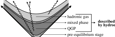
Figure 1: The various stages of a heavy ion collision.

Some photons are produced in the initial partonic collisions. These prompt photons can be calculated using zero temperature perturbative QCD, and they populate the high energy part of the spectrum. Then comes a pre-equilibrium phase, which is usually thought to be very short and very poor in quarks and anti-quarks, so that photon production in this phase is neglected. In scenarios with a quark-gluon plasma, this is followed by the plasma phase, which produces photons at a rate calculable using equilibrium thermal field theory (TFT). Indeed, a local equilibrium is usually assumed for the plasma phase, and the local rate calculated using TFT is then folded in an hydrodynamical evolution code [1, 2, 3, 4] in order to perform the integration over space-time. After the confinement phase transition, the system becomes a hadronic gas (there can be a mixed phase if the phase transition is first order), for which TFT (now with hadronic degrees of freedom) can also be used in order to compute the photon rate. Finally the system freezes out and the only photons that are produced afterwards are decay products of hadrons. The photon yield observed in detectors is the sum of all these contributions. In the rest of this talk, I focus on photons produced in the QGP phase, and on the TFT techniques used in order to compute their rate.

In order to compute the photon production rate in a QGP, one can proceed as follows: make the list of the processes contributing up to a given order, add up the corresponding amplitudes, square this sum and integrate out all the particles but the photon, properly weighted by the appropriate statistical distribution. However, this method becomes rapidly cumbersome since one must track by hand the statistical factors, and the interference terms. TFT provides a convenient alternative to this approach, which has the advantage of taking care automatically of the statistical factors and interferences. In this approach, the photon production rate is expressed in terms of the imaginary part of the retarded polarization tensor [5, 6]:

$${{\omega\frac{dN_{\gamma}}{dtdVd^{3}{\boldsymbol{q}}}}}=\frac{1}{(2\pi)^{3}}\frac{1}{e^{\omega/T}-1}\;{{\rm Im}\,\Pi_{\rm ret}{{}^{\mu}{}_{\mu}}(\omega,{\boldsymbol{q}})}\;.$$ (1)

The calculation of this retarded imaginary part can be simplified by the use of cutting rules [7], and it is the sum over all the possible cuts that takes care of the interference terms. Note that a similar formula exists for lepton pairs, for which one needs to compute the polarization tensor of a massive photon (i.e. $Q^{2}\equiv\omega^{2}-{\boldsymbol{q}}^{2}>0$).

2 HISTORY

The calculation of thermal photon and dilepton rates has a long and tortuous history. The dilepton rate due to the Drell-Yan process (see the diagram on the left of figure 2) was evaluated in a QGP in [8].

Figure 2: Real processes contributing to photon and dilepton production up to ${\cal O}(\alpha_{s})$. Virtual corrections to the first process also contribute at this order.

Corrections of order ${\cal O}(\alpha_{s})$ were considered shortly afterwards, and two problems became apparent. If one tries to calculate the dilepton rate ($Q^{2}>0$) in a plasma of massless quarks and gluons, each individual cut contributing to eq. (1) contains a mass singularity, and it is only after a careful summation of all the real and virtual corrections that one gets a finite result [9, 10, 11]. This is nothing but a manifestation of a general property noted in [12]. If one then tries to take the limit of real photons ($Q^{2}\to 0^{+}$) in the above formula, a new singularity appears since there are some terms that behave like ${\rm Im}\,\Pi_{\rm ret}(\omega,{\boldsymbol{q}})\propto\alpha\alpha_{s}\ln(\omega T/Q^{2})$ at small $Q^{2}$.

The latter problem was resolved by the resummation of Hard Thermal Loops (HTL). HTL are one-loop leading thermal corrections that have the same order of magnitude as their bare counterpart when their external momenta are soft (i.e. of ${\cal O}(\sqrt{\alpha_{s}}T)$). They were known for quite some time in the case of 2-point functions [13, 14], but a systematic gauge invariant resummation was only proposed in 1990 by [15, 16]. In the present case, the logarithmic singularity at $Q^{2}\to 0$ is due to the exchange of a soft massless quark. This singularity is screened by the resummation of the HTL correction to the quark propagator, which gives the quark a thermal mass $m_{\rm q}$ of order $m_{\rm q}\sim\sqrt{\alpha_{s}}T$. Taking into account this thermal correction to the quark propagator solves the problem and leads to a finite photon polarization tensor [17, 18]. For hard photons, it reads:

$${\rm Im}\,\Pi_{\rm ret}{}^{\mu}{}_{\mu}(\omega,{\boldsymbol{q}})=4\pi{\frac{5\alpha\alpha_{s}}{9}}T^{2}\left[\ln\left(\frac{\omega T}{m_{\rm q}^{2}}\right)-\frac{1}{2}-\gamma_{{}_{E}}+\frac{7}{3}\ln(2)+\frac{\zeta^{\prime}(2)}{\zeta(2)}\right]\;.$$ (2)

Note that throughout this talk the mass $m_{\rm q}$ is defined to be the asymptotic quark thermal mass, i.e. $m_{\rm q}^{2}=\pi\alpha_{s}C_{f}T^{2}$ with $C_{f}\equiv(N_{c}^{2}-1)/2N_{c}$. The numerical factor $5/9$ is the sum of the quark electric charges squared for $2$ flavors (u and d); for $3$ flavors (u, d and s), this factor should be replaced by $6/9$. Regarding the infrared problem, one can see that $Q^{2}$ is replaced by $m_{\rm q}^{2}$ in the logarithm as soon as $Q^{2}$ becomes small compared to $m_{\rm q}^{2}$.

This was thought to be the final answer for the photon and dilepton rates at ${\cal O}(\alpha_{s})$, until it became clear that some formally higher order processes are in fact strongly enhanced by collinear singularities. This was first realized for soft photon production by quark bremsstrahlung [19, 20] (left diagram of figure 3). The diagram on the right of figure 3 shares the same property, but contributes significantly only to hard photon production [21], due to phase-space suppression in the case of soft photons. Note that a naive power counting would indicate that these two diagrams contribute to ${\cal O}(\alpha_{s}^{2})$. A common property of these two diagrams is that they have an off-shell quark next to the vertex where the photon is emitted, and that the virtuality of this quark can become very small if the photon is emitted forward.

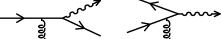
Figure 3: Two processes that are promoted to ${\cal O}(\alpha_{s})$ by collinear singularities.

Again, it is the quark thermal mass $m_{\rm q}$ that prevents these diagrams from being truly singular. However, contrary to the ${\cal O}(\alpha_{s})$ diagrams, the singularity is linear instead of logarithmic, and brings a factor $T^{2}/m_{\rm q}^{2}$. Combined with the $\alpha_{s}^{2}$ that comes from the vertices, these diagrams turn out to be also of order ${\cal O}(\alpha_{s})$. In [20] and [21], their contribution was derived semi-analytically, with a prefactor that was evaluated numerically. [22] and [23] independently pointed out an erroneous factor $4$ in this numerical prefactor. Finally, it was realized that it can be calculated in closed form [24, 25]. For 3 colors and 2 light quark flavors, the ${\cal O}(\alpha_{s})$ contribution of these two diagrams is exactly:

$${\rm Im}\,\Pi_{\rm ret}{}^{\mu}{}_{\mu}(\omega,{\boldsymbol{q}})=\frac{32}{3\pi}\,\frac{5\alpha\alpha_{s}}{9}\left[\pi^{2}\frac{T^{3}}{\omega}+\omega T\right]\;.$$ (3)

In this formula, the term in $1/\omega$ dominates for soft photons and comes from the bremsstrahlung diagram, while the term in $\omega$ comes from the second diagram. Because of this term in $\omega$, this process turns out to dominate the rate of very hard photons ($\omega\gg T$). This was confirmed by more realistic evaluations that included this local rate into an hydrodynamical evolution code, and there is some speculation that these hard thermal photons could be part of the excess of direct photons observed by the WA98 experiment at SPS [1, 2, 3, 26, 27, 28] (see also [29]). Note that it is only by accident if this result is so simple. For 3 colors and 3 light flavors, the same quantity can still be calculated in closed form (note that the energy dependence is the same), but the prefactor is much more involved:

$${\rm Im}\,\Pi_{\rm ret}{}^{\mu}{}_{\mu}(\omega,{\boldsymbol{q}}) = \frac{32}{3\pi}\left[1+\frac{5\pi^{2}}{36}+{\ln\left(\frac{\sqrt{2}}{3}\right)}-\frac{55}{12}\ln^{2}(2)+\frac{10}{3}\ln(2)\ln(3)\right.$$ (4)

$$\quad\qquad-\left.\frac{5}{3}{\rm Li}_{2}\left(\frac{3}{4}\right)-\frac{5}{3}{\rm Li}_{2}\left(-\frac{1}{2}\right)\right]\,\frac{6\alpha\alpha_{s}}{9}\left[\pi^{2}\frac{T^{3}}{\omega}+\omega T\right]\;.$$

It is also worth mentioning at this point that the purely numerical prefactor is a function of the ratio of the quark thermal mass $m_{\rm q}$ to the gluon Debye mass $m_{\rm debye}$ (the Debye mass quantifies the effective range of strong interactions when they are screened by medium effects, and it is also of ${\cal O}(\sqrt{\alpha_{s}}T)$). In the HTL framework, this ratio is a constant independent of the coupling and temperature, that depends only on the number of colors and flavors; for $3$ colors and $N_{f}$ flavors, this ratio is $m_{\rm q}/m_{\rm debye}=\sqrt{2/(6+N_{f})}$.

3 LPM EFFECT

Given the enhancement in the diagrams of figure 3, one may wonder if there are formally higher order diagrams that also end up contributing to the same order ${\cal O}(\alpha_{s})$. This was partly answered in [30] where the resummation of a collisional width $\Gamma\sim\alpha_{s}T\ln(1/\alpha_{s})$ on the quarks in the calculation of the diagrams of figure 3 showed some sensitivity to this parameter at leading order, thereby indicating that an infinite series of diagrams must be resummed in order to fully determine the ${\cal O}(\alpha_{s})$ photon rate.

In order to explain the issue in more physical terms, it is convenient to define the concept of photon formation time. Let me assume that a virtual quark of momentum $R\equiv P+Q$ splits into an on-shell quark of momentum $P$ and a photon of momentum $Q$. The photon formation time can be identified with the lifetime of the virtual quark, which is itself related to its virtuality by the uncertainty principle. For a small $Q^{2}$, a simple calculation gives:

$$t_{{}_{F}}^{-1}\sim{\delta E}=r_{0}-\sqrt{{\boldsymbol{r}}^{2}+m_{\rm q}^{2}}\approx\frac{\omega}{2p_{0}r_{0}}\left[{\boldsymbol{p}}_{\perp}^{2}+{m_{\rm q}^{2}}+\frac{Q^{2}}{\omega^{2}}p_{0}r_{0}\right]\;,$$ (5)

where the 3-momentum of the photon defines the longitudinal axis. Note that the collinear enhancement in the diagrams of figure 3, due to the small virtuality of the quark that emits the photon, can be rephrased by saying that it is due to a large photon formation time. Similarly, the sensitivity to the collisional width found in [30] occurs if the photon formation time is of the same order or larger than the quark mean free path between two soft collisions (this mean free path $\lambda$ is the inverse of the width $\Gamma$). This phenomenon is nothing but a manifestation of the Landau Pomeranchuk Migdal (LPM) effect [31, 32, 33].

The precise nature of the multiple scattering diagrams that must be resummed depends in fact on the range of the interactions in the medium. Indeed, if the range $\ell$ of the interactions is much shorter than the mean free path, it is easy to check that only ladder topologies are important, in which all the successive scatterings are independent of one another, as illustrated in figure 4.

Figure 4: A ladder correction to bremsstrahlung.

Indeed, the condition $\ell\ll\lambda$ suppresses diagrams with crossed gluons. On the contrary, if there are long range interactions in the system, for which $\ell\gtrsim\lambda$, then arbitrarily complicated topologies can a priori contribute. It was found in [34] that if one considers contributions to the photon polarization tensor topology by topology, then there can be a sensitivity to interaction ranges as long as the magnetic scale $1/\alpha_{s}T$ (for a review of the relevant scales and associated physics in a QGP, see [35]), which would render the problem practically intractable.

A considerable progress was made recently in [36], in which it was shown that there are infrared cancellations between diagrams of different topologies, and that these cancellations remove any sensitivity to the magnetic scale. Physically, this cancellation can be interpreted as the fact that ultrasoft scatterings are not efficient in order to induce the production of a photon. As a consequence, only the ladder family of diagrams needs to be resummed in order to obtain the complete leading ${\cal O}(\alpha_{s})$ photon rate. The resummation of this series of diagram can then be performed in two steps summarized in figure 5.

Figure 5: Resummation of ladder diagrams.

The first one is a Dyson equation for the photon polarization tensor, whose explicit form is [36, 37, 38]:

$${\rm Im}\,\Pi_{\rm ret}{}^{\mu}{}_{\mu}(Q)\approx{\alpha N_{c}}\int_{-\infty}^{+\infty}\!\!dp_{0}\,[n_{{}_{F}}(r_{0})-n_{{}_{F}}(p_{0})]\;\frac{p_{0}^{2}+r_{0}^{2}}{(p_{0}r_{0})^{2}}\,{\rm Re}\int\frac{d^{2}{\boldsymbol{p}}_{\perp}}{(2\pi)^{2}}\;{\boldsymbol{p}}_{\perp}\cdot{\boldsymbol{f}}({\boldsymbol{p}}_{\perp})\;,$$ (6)

with $r_{0}\equiv p_{0}+q_{0}$, $n_{{}_{F}}(p_{0})\equiv 1/(\exp(p_{0}/T)+1)$ the Fermi-Dirac statistical weight, and where the dimensionless function ${\boldsymbol{f}}({\boldsymbol{p}}_{\perp})$ denotes the resummed vertex between the quark line and the transverse modes of the photon (this is represented by the shaded vertex in the above pictures). In the Dyson equation, this function is dotted into a bare vertex, which is proportional to ${\boldsymbol{p}}_{\perp}$. The second equation, that determines the value of ${\boldsymbol{f}}({\boldsymbol{p}}_{\perp})$, is a Bethe-Salpeter equation that resums all the ladder corrections [36, 37, 38]:

$$\frac{i}{t_{{}_{F}}}{\boldsymbol{f}}({\boldsymbol{p}}_{\perp})=2{\boldsymbol{p}}_{\perp}+4\pi\alpha_{s}C_{f}T\!\!\int\frac{d^{2}{\boldsymbol{l}}_{\perp}}{(2\pi)^{2}}\,{\cal C}({\boldsymbol{l}}_{\perp})\,[{\boldsymbol{f}}({\boldsymbol{p}}_{\perp}+{\boldsymbol{l}}_{\perp})-{\boldsymbol{f}}({\boldsymbol{p}}_{\perp})]\;,$$ (7)

where $t_{{}_{F}}$ is the time defined in eq. (5) and where the collision kernel has the following expression: ${\cal C}({\boldsymbol{l}}_{\perp})={m^{2}_{\rm debye}}/{{\boldsymbol{l}}_{\perp}^{\ 2}}({{\boldsymbol{l}}_{\perp}^{\ 2}+{m^{2}_{\rm debye}}})$ [24]. Note that in the Dyson equation, the quark propagators should be dressed in a way compatible with the resummation performed for the vertex, in order to preserve the gauge invariance. It is this dressing on the quark propagators which is responsible for the term $-{\boldsymbol{f}}({\boldsymbol{p}}_{\perp})$ under the integral in eq. (7). From this integral equation, it is easy to see that each extra rung in the ladder contributes a correction of order $\alpha_{s}Tp_{0}r_{0}/\omega m_{\rm q}^{2}$, in which the $\alpha_{s}$ drops out. Therefore, all these corrections contribute to ${\cal O}(\alpha_{s})$ to the photon rate. Note again that the only parameters of the QGP that enter in this equation are the quark thermal mass $m_{\rm q}$ and the Debye screening mass $m_{\rm debye}$. This integral equation was solved numerically in [37], and the results are displayed in figure 6.

Figure 6: ${\cal O}(\alpha_{s})$ contributions to the photon production rate in a QGP. The parameters used in this plot are $\alpha_{s}=0.3$, 3 colors, 2 flavors and $T=1$ GeV.

In this plot, ‘LPM’ denotes the contribution of all the multiple scattering diagrams, while ‘$2\to 2$’ denotes the processes of figure 2. The single scattering diagrams (figure 3) are also given so that one can appreciate the suppression due to the LPM effect.

4 DILEPTON PRODUCTION

Dilepton production basically suffers from the same problems, and the solution follows the same path. Two differences are worth mentioning here. First of all, the Drell-Yan process $q\bar{q}\to\gamma^{*}\to l^{+}l^{-}$ contributes if $Q^{2}\geq 4m_{\rm q}^{2}$. In addition, virtual photons have a physical longitudinal mode that contributes to the rate of lepton pairs. The Drell-Yan process has been evaluated in [8], and the $2\to 2$ processes have been evaluated in [11].

For photon invariant masses of order $Q^{2}\sim\alpha_{s}T^{2}$ or smaller, one expects also important contributions from multiple scattering diagrams. One must now keep track of the non-zero $Q^{2}$, and include also the contribution of the photon longitudinal mode. This is easily done by performing the following substitution in eq. (6) [39]:

$$\frac{p_{0}^{2}+r_{0}^{2}}{(p_{0}r_{0})^{2}}\,{\boldsymbol{p}}_{\perp}\cdot{\boldsymbol{f}}({\boldsymbol{p}}_{\perp})\to\frac{p_{0}^{2}+r_{0}^{2}}{(p_{0}r_{0})^{2}}\,{\boldsymbol{p}}_{\perp}\cdot{\boldsymbol{f}}({\boldsymbol{p}}_{\perp})+\frac{2}{\sqrt{|p_{0}r_{0}|}}\frac{Q^{2}}{q_{0}^{2}}\,g({\boldsymbol{p}}_{\perp})\;,$$ (8)

where the function $g({\boldsymbol{p}}_{\perp})$, which describes the coupling between the quark line and the longitudinal photon, obeys an integral equation similar to eq. (7) [39]:

$$\frac{i}{t_{{}_{F}}}{g}({\boldsymbol{p}}_{\perp})=2\sqrt{|p_{0}r_{0}|}+4\pi\alpha_{s}C_{f}T\int\frac{d^{2}{\boldsymbol{l}}_{\perp}}{(2\pi)^{2}}{\cal C}({\boldsymbol{l}}_{\perp})[{g}({\boldsymbol{p}}_{\perp}+{\boldsymbol{l}}_{\perp})-{g}({\boldsymbol{p}}_{\perp})]\;.$$ (9)

Note that the contribution of the longitudinal mode of the photon vanishes trivially when $Q^{2}\to 0$, as it should. This new integral equation can also be solved numerically, and the resulting dilepton rate (for the same parameters as in figure 6 and a total energy of the pair set to $\omega=5~{}$GeV) is plotted in figure 7.

Figure 7: ${\cal O}(\alpha_{s})$ contributions to the dilepton production rate in a QGP.

One can see that the multiple scattering corrections are important for all pair masses below the threshold of the Drell-Yan process. Note also that the threshold of the tree-level process is completely washed out when multiple rescatterings are resummed.

5 QUASIPARTICLE MODELS

We have emphasized several times the fact that the only properties of the QGP that these rates depend on are the quark thermal mass $m_{\rm q}$ and the Debye mass $m_{\rm debye}$. So far, these two masses have been taken in the HTL approximation, for which the ratio of the two masses is independent of $T$ and $\alpha_{s}$. However, simple arguments indicate that this ratio cannot remain constant when the mass $m_{\rm q}$ becomes large, which may happen at moderate temperatures for which the coupling constant is rather large. Indeed, the Debye screening is due to the possibility for a test charge to polarize the medium surrounding it in order to screen its charge. This process becomes difficult to achieve when the quasiparticles in the medium become very heavy, and for this reason $m_{\rm debye}$ should become very small if $m_{\rm q}$ increases. This is indeed what one finds by calculating the Debye mass at 1-loop, with massive particles running in the loop.

In practice, one could obtain the mass $m_{\rm q}$ from a quasiparticle fit to the lattice entropy, as has been done in [40]. This is illustrated in figure 8.

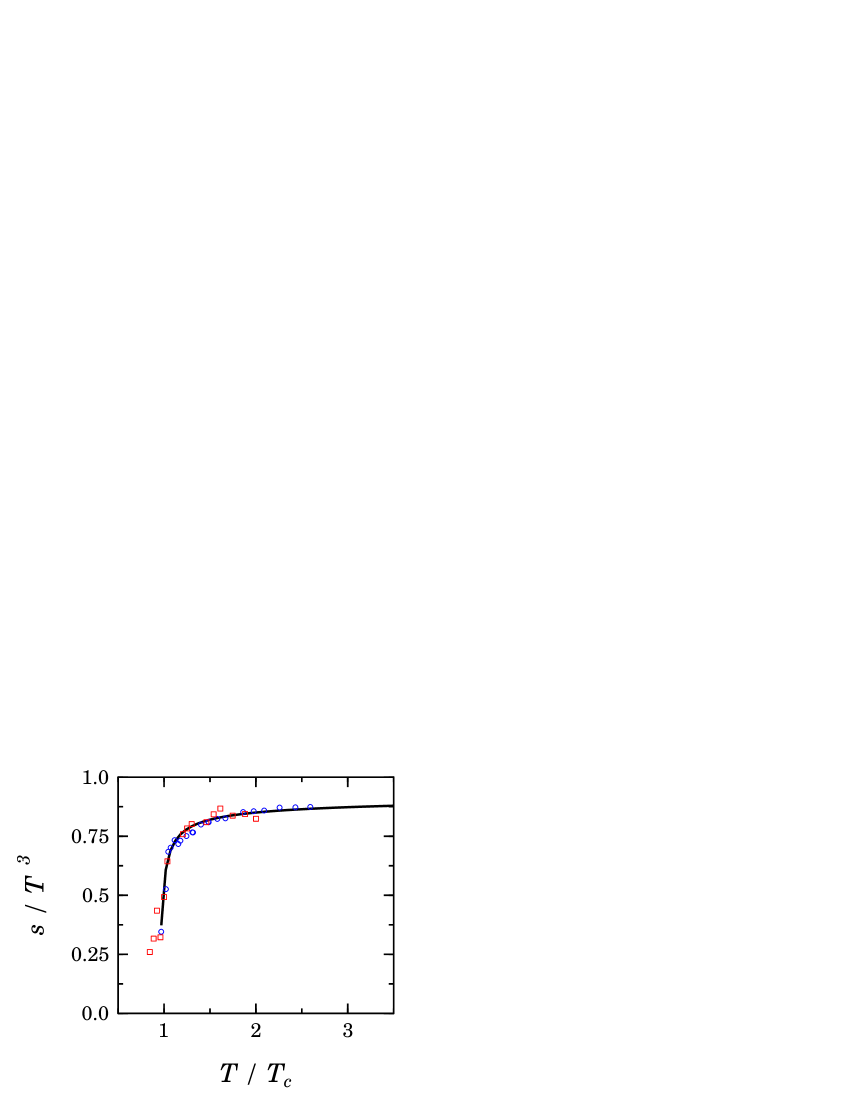
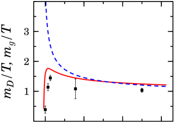
Figure 8: Extraction of $m_{\rm q}$ from a fit of the lattice entropy, and comparison of the resulting $m_{\rm debye}$ with the Debye mass measured on the lattice (see the text for more details).

On the left plot, one can see that this fit reproduces perfectly the entropy measured on the lattice, even for temperatures very close to the critical temperature $T_{c}$. The quasiparticle mass (here it is a gluon mass $m_{g}$, but this is proportional to $m_{\rm q}$) needed for that fit is shown by a dashed line in the right plot, and one can see that it becomes very large near $T_{c}$. The solid line is the Debye mass calculated at 1-loop, with the mass obtained from the previous fit used for the particle in the loop. The dots are the values of the Debye mass measured on the lattice, and one can see that at least the trend is remarkably well predicted by this very simple model. Since photon rates often need to be evaluated at temperatures that are not very large compared to $T_{c}$, it could be important to take the values of $m_{\rm q}$ and $m_{\rm debye}$ from this model rather than from the HTL approximation.

6 LATTICE CALCULATIONS

Recently appeared the first attempt to calculate directly on the lattice the production rate of dileptons in a quark-gluon plasma. In fact, the principle of this calculation has been known for a long time: one should start from the Euclidean correlator of two vector currents $\Pi(\tau,{\boldsymbol{x}})\equiv\left<j_{\mu}(0,{\boldsymbol{0}})j^{\mu}(\tau,{\boldsymbol{x}})\right>$, where $\tau\in[0,1/T]$ is the Euclidean time. Next, one obtains $\Pi(\tau,{\boldsymbol{q}})$ by a Fourier transformation of the spatial coordinates, and the imaginary part of the real time self-energy is then related to this object by a simple spectral representation:

$${\Pi(\tau,{\boldsymbol{q}})}=\int_{0}^{\infty}\!\!{d\omega}\,{{\rm Im}\,\Pi_{\rm ret}{}^{\mu}{}_{\mu}(\omega,{\boldsymbol{q}})}\,\frac{\cosh(\omega(\tau-1/2T))}{\sinh(\omega/2T)}\;.$$ (10)

In fact, this equation uniquely defines ${\rm Im}\,\Pi_{\rm ret}{}^{\mu}{}_{\mu}(\omega,{\boldsymbol{q}})$ if $\Pi(\tau,{\boldsymbol{q}})$ is known for all $\tau\in[0,1/T]$ and if one prescribes the behavior of the solution at large $\omega$.

The main problem in lattice calculations is that one knows the function $\Pi(\tau,{\boldsymbol{q}})$ only on the discrete points of the lattice, which prevents from determining uniquely the solution. This problem has been reconsidered recently using the Maximum Entropy Method [41, 42], which is a way to take into account prior knowledge about the solution (positivity, behavior at the origin, etc…) in order to determine the most probable solution compatible with the lattice data and with this a priori information. The result obtained for static dileptons (${\boldsymbol{q}}=0$) via this method is displayed in the figure 9, for two different values of the temperature. Note that this is a quenched lattice simulation.

Figure 9: Lattice result for the production rate of static dileptons.

This result displays several interesting properties. At energies above $4T$, the full rate is very close to the contribution of the Born term, while at energies smaller than $3T$ it drops to extremely small values. In addition, when plotted against $\omega/T$, the curves for the two temperatures fall almost on top of one another, indicating that the result scales like a universal function of $\omega/T$, at least within the errors.

In fact, the suppression at small $\omega$ has attracted a lot of interest because it is not what one would expect from perturbation theory: the resummation of thermal masses would indeed produce a drop of the Born term because of threshold effects, but there are some higher order processes that do not have a threshold and that should fill the spectrum at small $\omega$. As of now, there are arguments indicating that both the perturbative calculations and the lattice calculation are incorrect at small $\omega$. If one evaluates eq. (10) at $\tau=1/2T$, one gets a sum rule: $\int_{0}^{\infty}{d\omega}{{\rm Im}\,\Pi_{\rm ret}{}^{\mu}{}_{\mu}(\omega,{\boldsymbol{q}})}/{\sinh(\omega/2T)}=\Pi(1/2T,{\boldsymbol{q}})<\infty$, which is violated by all the existing perturbative calculations (they give an infinite result) because none of them includes the strong dissipative effects that appear when one enters in the hydrodynamical regime ($\omega\to 0$).

On the other hand [43], from the electric conductivity: $\sigma_{\rm el}=\lim_{\omega\to 0}{{{\rm Im}\,\Pi_{\rm ret}(\omega,{0})}/{6\omega}}$, one obtains ${\rm Im}\,\Pi_{\rm ret}(\omega,{0})\propto\omega$ when $\omega\to 0$. This implies that the static dilepton rate should diverge when $\omega\to 0$. Unless the electric conductivity in quenched QCD is nearly zero for some (yet to be explained) reason, the lattice dilepton rate disagrees with this prediction at small $\omega$. Note that ‘small’ in these considerations means an $\omega$ small enough to be in the hydrodynamical regime, i.e. $\omega\lesssim g_{s}^{4}T$. In a strong coupling theory, this regime could start as early as $\omega\sim T$.

7 CONCLUSIONS

The full ${\cal O}(\alpha_{s})$ photon and dilepton rates have now been calculated using thermal QCD. This required to resum all the diagrams involving multiple rescatterings as it turns out that the LPM suppression plays a role at this order. A possible improvement of this perturbative calculation could come via the use of quasiparticle models adjusted to reproduce thermodynamical quantities determined on the lattice, in order to get more realistic values for the various mass parameters that describe the internals of the QGP.

Another recent development is the direct lattice evaluation of the static dilepton rate. More work is still needed in this area in order to fully understand the discrepancy with the perturbative approach at low energy, and also to extend this program to real photons.

Finally, one should also mention that the way the pre-equilibrium phase is treated (or, more accurately, ignored) is probably not correct as there are indications that the kinetic equilibration time might be as long as a few fermis [44]. Determining how quarks are dynamically generated from the initial gluons is a topic that certainly deserves much more attention, and may influence strongly the photon yields on obtains at the end.

References

- [1] D.K. Srivastava, Eur. Phys. J. C 10, 487 (1999).
- [2] D.K. Srivastava, B. Sinha, Phys. Rev. C 64, 034902 (2001).
- [3] P. Huovinen, P.V. Ruuskanen, S.S. Rasanen, Phys. Lett. B 535, 109 (2002).
- [4] J. Alam, S. Sarkar, P. Roy, T. Hatsuda, B. Sinha, Annals Phys. 286, 159 (2001).
- [5] H.A. Weldon, Phys. Rev. D 28, 2007 (1983).
- [6] C. Gale, J.I. Kapusta, Nucl. Phys. B 357, 65 (1991).
- [7] F. Gelis, Nucl. Phys. B 508, 483 (1997).
- [8] L. McLerran, T. Toimela, Phys. Rev. D 31, 545 (1985).
- [9] R. Baier, B. Pire, D. Schiff, Phys. Rev. D 38, 2814 (1988).
- [10] T. Altherr, P. Aurenche, T. Becherrawy, Nucl. Phys. B 315, 436 (1989).
- [11] T. Altherr, P.V. Ruuskanen, Nucl. Phys. B 380, 377 (1992).
- [12] T.D. Lee, M. Nauenberg, Phys. Rev. 133, 1549 (1964).
- [13] V.V. Klimov, Sov. J. Nucl. Phys. 33, 934 (1981).
- [14] H.A. Weldon, Phys. Rev. D 26, 2789 (1982).
- [15] E. Braaten, R.D. Pisarski, Nucl. Phys. B 337, 569 (1990).
- [16] J. Frenkel, J.C. Taylor, Nucl. Phys. B 334, 199 (1990).
- [17] J.I. Kapusta, P. Lichard, D. Seibert, Phys. Rev. D 44, 2774 (1991).
- [18] R. Baier, H. Nakkagawa, A. Niegawa, K. Redlich, Z. Phys. C 53, 433 (1992).
- [19] P. Aurenche, F. Gelis, R. Kobes, E. Petitgirard, Phys. Rev. D 54, 5274 (1996).
- [20] P. Aurenche, F. Gelis, R. Kobes, E. Petitgirard, Z. Phys. C 75, 315 (1997).
- [21] P. Aurenche, F. Gelis, R. Kobes, H. Zaraket, Phys. Rev D 58, 085003 (1998).
- [22] A.K. Mohanty, Communication at the International Symposium in Nuclear Physics, December 18-22, 2000, Mumbai, India.
- [23] F.D. Steffen, M.H. Thoma, Phys. Lett. B 510, 98 (2001).
- [24] P. Aurenche, F. Gelis, H. Zaraket, JHEP 0205, 043 (2002).
- [25] P. Aurenche, F. Gelis, H. Zaraket, JHEP 0207, 063 (2002).
- [26] A.K. Chaudhuri, nucl-th/0012058.
- [27] A.K. Chaudhuri, T. Kodama, nucl-th/0203067.
- [28] M.M. Aggarwal et al., WA98 collaboration, Phys. Rev. Lett. 85, 3595 (2000).
- [29] Talks by A. Dumitru, J. Kapusta, S. Rasanen and H. Zaraket.
- [30] P. Aurenche, F. Gelis, H. Zaraket, Phys. Rev. D 62, 096012 (2000).
- [31] L.D. Landau, I.Ya. Pomeranchuk, Dokl. Akad. Nauk. SSR 92, 535 (1953).
- [32] L.D. Landau, I.Ya. Pomeranchuk, Dokl. Akad. Nauk. SSR 92, 735 (1953).
- [33] A.B. Migdal, Phys. Rev. 103, 1811 (1956).
- [34] P. Aurenche, F. Gelis, H. Zaraket, Phys. Rev. D 61, 116001 (2000).
- [35] Talk by D. Bödeker.
- [36] P. Arnold, G.D. Moore, L.G. Yaffe, JHEP 0111, 057 (2001).
- [37] P. Arnold, G.D. Moore, L.G. Yaffe, JHEP 0112, 009 (2001).
- [38] P. Arnold, G.D. Moore, L.G. Yaffe, JHEP 0206, 030 (2002).
- [39] P. Aurenche, F. Gelis, G.D. Moore, H. Zaraket, In preparation.
- [40] A. Peshier, B. Kampfer, O.P. Pavlenko, Phys. Rev. D 54, 2399 (1996).
- [41] F. Karsch, E. Laermann, P. Petreczky, S. Stickan, I. Wetzorke, Phys. Lett. B 530, 147 (2002).
- [42] Talks by M. Asakawa, K. Kanaya and F. Karsch.
- [43] G.D. Moore, Private communication.
- [44] R. Baier, A.H. Mueller, D. Schiff, D.T. Son, Phys. Lett. B 539, 46 (2002).