Quantum dynamics of phase transitions in broken symmetry $\lambda\,\phi^{4}$ field theory

Abstract

We perform a detailed numerical investigation of the dynamics of a single component broken symmetry $\lambda\,\phi^{4}$ field theory in 1+1 dimensions using a Schwinger-Dyson equation truncation scheme based on ignoring vertex corrections. In an earlier paper, we called this the bare vertex approximation (BVA). We assume the initial state is described by a Gaussian density matrix peaked around some non-zero value of $\langle\phi(0)\rangle$, and characterized by a single particle Bose-Einstein distribution function at a given temperature. We compute the evolution of the system using three different approximations: Hartree, BVA and a related 2PI-1/N expansion, as a function of coupling strength and initial temperature. In the Hartree approximation, the static phase diagram shows that there is a first order phase transition for this system. As we change the initial starting temperature of the system, we find that the BVA relaxes to a new final temperature and exhibits a second order phase transition. We find that the average fields thermalize for arbitrary initial conditions in the BVA, unlike the behavior exhibited by the Hartree approximation, and we illustrate how $\langle\phi(t)\rangle$ and $\langle\chi(t)\rangle$ depend on the initial temperature and on the coupling constant. We find that the 2PI-1/N expansion gives dramatically different results for $\langle\phi(t)\rangle$.

I Introduction

Recently there has been much effort in finding approximation schemes to study the dynamics of phase transitions that go beyond a leading order in large-N mean field theory approach. This is an important endeavor if one wants a first principles understanding of the dynamics of quantum phase transitions. In a previous set of papers, we studied in quantum mechanics Mihaila et al. (2001), as well as 1+1 dimensional field theory Blagoev et al. (2001), the validity of a $1/N$ motivated resummation scheme, which we called the bare vertex approximation (BVA).

The long-term goal of this work is finding approximation schemes which are accurate at the small values of N relevant to the case of realistic quantum field theories: N=4 for the linear sigma model, and N=2 for the Walecka model. In order to maximize the possible differences between approximation schemes we choose to study the O(N) model for $N=1$. Based on our previous studies of the quantum mechanical version of this model Mihaila et al. (2001) we expect that by increasing N the differences will diminish. This is due to the fact that the Schwinger-Dyson formalism is related, but not identical, with approximations based on the large-N expansion.

This paper presents the first quantum-mechanical dynamical calculation in 1+1 dimensions, using the BVA, of the explicitly broken symmetry case, where the order parameter at $t=0$ is non-zero. In 1+1 dimensions, it is known that there is no phase transition in this model except at zero temperature Griffiths (1972). On the other hand, in two dimensional systems having Berezinski-Kosterlitz-Thouless type transitions Berezinski (1970); Kosterlitz and Thouless (1973); Jose et al. (1977), the large-N expansion can give qualitatively good understanding of the correlation functions, even when it gives the wrong phase transition behavior Witten (1978). As the dimensions increase, the mean field critical behavior becomes exact in four dimensions and thus we expect that the approximation presented here should improve as we increase the dimensionality. Thus we should think of the model used here as a “toy” model for demonstrating some of the features expected to be true in 3+1 dimensions such as the restoration of symmetry breakdown at high temperatures and thermalization of correlation functions. The model we are ultimately interested in is the linear sigma model in 3+1 dimensions for the case of broken symmetry at finite temperature. This model we studied earlier using a large-N approximation Kennedy et al. (1996); Lampert (1996); Kluger et al. (1995). Since the BVA contains scattering contributions, it cures many of the problems associated with mean field methods. Here we are able to follow the evolution of the system through a phase transition and study the thermalization of the system. We illustrate in this paper the results of such calculations.

A parallel set of investigations by Berges et. al. Berges and Cox (2001); Aarts and Berges (2001, 2002); Berges (2002); Arts et al. , have looked at a related approximation based on the two-particle irreducible expansion (which they call 2PI-1/N). These investigators have pointed out that when there is broken symmetry, the BVA contains terms not included in the $1/N$ resummation at next to leading order. In this paper, we present the first quantum calculations which compare the BVA with the 2PI-1/N for the broken symmetry case. Recently we were able to show that for a classical finite temperature $\lambda\phi^{4}$ field theory in 1+1 dimensions, the BVA gave a better description of the time evolution of $\langle\phi(t)\rangle$ than the 2PI-1/N expansion and provided excellent agreement with exact Monte Carlo simulations Cooper et al. (2002); Blagoev et al. (2001).

In this paper we look at quantum evolutions in 1+1 dimensions, starting with a Gaussian density matrix, and study how the evolution of $\langle\phi(t)\rangle$ depends on the initial conditions and the value of the coupling constant. In the classical domain, the coupling constant dependence can be scaled out, which is not possible in the quantum case we consider here. Since we have not determined the effective potential in the BVA approximation, we rely on the Hartree approximation effective potential to guide our study. The Hartree potential however, indicates that the system should undergo a first order phase transition. In addition, in the Hartree approximation, the fields never thermalize. We find that the BVA cures these serious problems. In this paper, we show evolutions of the system as a function of the initial “temperature” parameter and the coupling constant, and, since in the BVA, the fields thermalize, we can follow the system through what appears to be a second order phase transition. We also compare our results with those of the 2PI-1/N expansion in the quantum domain, and find that the two approximations diverge dramatically for the behavior of $\langle\phi(t)\rangle$.

We derive the BVA equations for the general $N$-component $\lambda\,[\,\phi^{2}_{i}(x)\,]^{2}$ field theory in Sections II and III. We then specialize to the case $N=1$, and in Section IV, we derive the Hartree approximation phase diagram. In Section V, we discuss the initial conditions we choose for this problem. Numerical results are shown in Section VI, and conclusions discussed in Section VII.

II The classical action and time evolution in the BVA

The classical action for $\lambda\phi^{4}$ with $N$ fields ($i=1\ldots N$) is

$$S[\phi]=\int\mathrm{d}^{2}x\,\biggl{\{} \frac{1}{2}\,\Bigl{[}\partial_{\mu}\phi_{i}(x)\ \partial^{\mu}\phi_{i}(x)+\mu^{2}\,\phi_{i}^{2}(x)\Bigr{]}$$

$$-\frac{\lambda}{8N}\,[\,\phi^{2}_{i}(x)\,]^{2}-\frac{N\mu^{4}}{2\lambda}\,\biggr{\}}\>.$$ (1)

For the purposes of our resummation scheme which is motivated by $1/N$ considerations it is useful to consider the alternative action

$$S_{\text{cl}}[\phi_{i},\chi]=\int\mathrm{d}^{2}x\,\biggl{\{} \frac{1}{2}\,\Bigl{[}\partial_{\mu}\phi_{i}(x)\ \partial^{\mu}\phi_{i}(x)-\chi(x)\,\phi_{i}^{2}(x)\Bigr{]}$$

$$+\frac{N}{\lambda}\,\Bigl{[}\,\frac{\chi^{2}(x)}{2}+\mu^{2}\,\chi(x)\,\Bigr{]}\,\biggr{\}}\>,$$ (2)

which leads to the Heisenberg equations of motion

$$\left[\,\Box+\chi(x)\,\right]\,\phi_{i}(x)=0\>,$$ (3)

and the constraint (“gap”) equation for $\chi(x)$

$$\chi(x)=-\mu^{2}+\frac{\lambda}{2N}\,\phi_{i}(x)\phi_{i}(x)\>.$$ (4)

Throughout this paper, we use the Einstein summation convention for repeated indices.

The BVA truncation scheme of the Schwinger-Dyson equations is most easily obtained from the 2PI effective action Cornwall et al. (1974); Luttinger and Ward (1960); Baym (1962). Other approaches leading to these equations are found in Mihaila et al. (2001); Arts et al. . Using the extended fields notation, $\phi_{\alpha}(x)=[\chi(x),\phi_{1}(x),\phi_{2}(x),\ldots,\phi_{N}(x)]\>,$ the effective action for the evolution can be written as:

$$\Gamma[\phi_{\alpha},G]\ =\ S_{\text{cl}}[\phi_{\alpha}]+\frac{i}{2}{\rm Tr}\ln[\,G^{-1}\,]$$

$$+\frac{i}{2}{\rm Tr}[\,G_{0}^{-1}\,G\,]+\Gamma_{2}[G]\>,$$ (5)

where $\Gamma_{2}[G]$ is the generating functional of the 2-PI graphs, and the classical action in Minkowski space is

$$S_{\text{cl}}[\phi_{\alpha}]=\int d^{2}x\,\biggl{\{} -\frac{1}{2}\phi_{i}(x)\,[\,\Box+\chi(x)\,]\,\phi_{i}(x)$$

$$+\frac{\chi^{2}(x)}{2g}+\frac{\mu^{2}}{g}\chi(x)\,\biggr{\}}\>.$$ (6)

Here and in what follows we let $g=\lambda/N$.

The integrals and delta functions $\delta_{\mathcal{C}}(x,x^{\prime})$ are defined on the closed time path (CTP) contour, which incorporates the initial value boundary condition Schwinger (1961); Keldysh (1964); Mahanthappa (1963a, b). The approximations we are studying include only the two-loop contributions to $\Gamma_{2}$.

The Green function $G^{-1}_{0\,\alpha\beta}[\phi](x,x^{\prime})$ is defined as follows:

$$G_{0\,\alpha\beta}^{-1}[\phi](x,x^{\prime}) = -\frac{\delta^{2}S_{\text{cl}}}{\delta\phi_{\alpha}(x)\,\delta\phi_{\beta}(x^{\prime})}$$ (7)

$$= \begin{pmatrix}D^{-1}_{0}(x,x^{\prime})&\bar{K}_{0\,j}^{-1}(x,x^{\prime})\\ K_{0\,i}^{-1}(x,x^{\prime})&G_{0\,ij}^{-1}(x,x^{\prime})\end{pmatrix}\>,$$

where

$$D_{0}^{-1}(x,x^{\prime})=-\,g\,\delta_{\mathcal{C}}(x,x^{\prime})\>,$$

$$G_{0\,ij}^{-1}[\chi](x,x^{\prime})=[\,\Box+\chi(x)\,]\,\delta_{ij}\delta_{\mathcal{C}}(x,x^{\prime})\>,$$

$$K_{0\,i}^{-1}[\phi](x,x^{\prime})=\bar{K}_{0\,i}^{-1}[\phi](x,x^{\prime})=\phi_{i}(x)\,\delta_{\mathcal{C}}(x,x^{\prime})\>.$$

The exact Green function $G_{\alpha\beta}[j](x,x^{\prime})$ is defined by:

$$G_{\alpha\beta}[j](x,x^{\prime})=\begin{pmatrix}D(x,x^{\prime})&K_{j}(x,x^{\prime})\\ \bar{K}_{i}(x,x^{\prime})&G_{ij}(x,x^{\prime})\end{pmatrix}\>,$$

The exact equations following from the effective action Eq. (5), are:

$$[\,\Box+\chi(x)\,]\,\phi_{i}(x)+K_{i}(x,x)/i=0\>,$$ (8)

$$\chi(x)=-\mu^{2}+\frac{g}{2}\sum_{i}\bigl{[}\,\phi_{i}^{2}(x)+G_{ii}(x,x)/i\,\bigr{]}\>,$$

and

$$G_{\alpha\beta}^{-1}(x,x^{\prime})=G_{0\,\alpha\beta}^{-1}(x,x^{\prime})+\Sigma_{\alpha\beta}(x,x^{\prime})\>,$$ (9)

where

$$\Sigma_{\alpha\beta}(x,x^{\prime}) = \frac{2}{i}\,\frac{\delta\Gamma_{2}[G]}{\delta G_{\alpha\beta}(x,x^{\prime})}$$ (10)

$$= \begin{pmatrix}\Pi(x,x^{\prime})&\Omega_{j}(x,x^{\prime})\\ \bar{\Omega}_{i}(x,x^{\prime})&\Sigma_{ij}(x,x^{\prime})\end{pmatrix}\>.$$

In the BVA, we keep in $\Gamma_{2}[G]$ only the graphs shown in Fig. 1, which is explicitly

$$\Gamma_{2}[G]=-\frac{1}{4}\iint\mathrm{d}x\mathrm{d}y\Bigl{[} G_{ij}(x,y)G_{ji}(y,x)D(x,y)$$ (11)

$$+2\bar{K}_{i}(x,y)K_{j}(x,y)G_{ij}(x,y)\Bigr{]}\>.$$

The self-energy, given in Eq. (10), then reduces to:

$$\Pi(x,x^{\prime}) =\frac{i}{2}\,G_{mn}(x,x^{\prime})\,G_{mn}(x,x^{\prime})\>,$$ (12)

$$\Omega_{i}(x,x^{\prime}) =i\,\bar{K}_{m}(x,x^{\prime})\,G_{mi}(x,x^{\prime})\>,$$

$$\bar{\Omega}_{i}(x,x^{\prime}) =i\,\bar{K}_{m}(x,x^{\prime})\,G_{mi}(x,x^{\prime})\>,$$

$$\Sigma_{ij}(x,x^{\prime}) =i\,[\,G_{ij}(x,x^{\prime})\,D(x,x^{\prime})+\bar{K}_{i}(x,x^{\prime})\,K_{j}(x,x^{\prime})\,]\,.$$

As discussed in detail in Ref. Arts et al. , the second graph in Fig. 1 is proportional to $1/N^{2}$ and is ignored in the 2PI-1/N expansion. Our recent simulations in the classical domain showed that the BVA gave a more accurate determination of $\langle\phi(t)\rangle$, and we will concentrate in this paper on the BVA except to point out with explicit results that in the quantum domain the differences between the BVA and the 2PI-1/N expansion grow with increasing coupling constant $g$ (for the case $N=1$ studied here) and that unlike the BVA, the 2PI-1/N expansion does not track the average of the Hartree result.

Figure 1: Graphs included in the 2PI effective action $\Gamma_{2}$.

III Update equations for the Green functions

We notice from the definitions of the matrices representing $G_{\alpha\beta}(x,x^{\prime})$ and $G_{\alpha\beta}^{-1}(x,x^{\prime})$, that the matrix elements are not inverses of one another, but instead satisfy schematically:

$$D^{-1}D+\bar{K}_{k}^{-1}\bar{K}_{k} =\delta_{\mathcal{C}}\>,$$ (13)

$$K_{i}^{-1}D+G_{ik}^{-1}\bar{K}_{k} =0$$

$$D^{-1}K_{j}+\bar{K}_{k}^{-1}G_{kj} =0\>,$$

$$K_{i}^{-1}K_{j}+G_{ik}^{-1}G_{kj} =\delta_{ij}\delta_{\mathcal{C}}\>.$$

Inverting Eq. (9), we find:

$$D(x,x^{\prime}) = -g\,\delta_{\mathcal{C}}(x,x^{\prime})+g\,\int_{\mathcal{C}}\mathrm{d}x_{1}\ \Pi^{\prime}(x,x_{1})\ D(x_{1},x^{\prime})\>,$$ (14)

$$G_{ij}(x,x^{\prime}) = G_{0\,ij}(x,x^{\prime})\delta_{ij}-\int_{\mathcal{C}}\mathrm{d}x_{1}\int_{\mathcal{C}}\mathrm{d}x_{2}\ G_{0\,ik}(x,x_{1})\,\Sigma_{kl}^{\prime}(x_{1},x_{2})\ G_{lj}(x_{2},x^{\prime})\>,$$ (15)

$$K_{i}(x,x^{\prime}) = -\int_{\mathcal{C}}\mathrm{d}x_{1}\int_{\mathcal{C}}\mathrm{d}x_{2}\ \Bigl{[}D_{0}^{-1}+\Pi\Bigr{]}^{-1}\!\!(x,x_{1})\,\Bigl{[}\bar{K}_{0\,k}^{-1}+\Omega_{k}\Bigr{]}(x_{1},x_{2})\,G_{ki}(x_{2},x^{\prime})\>,$$ (16)

with

$$\Pi^{\prime}(x,x^{\prime}) = \Pi(x,x^{\prime})-\int_{\mathcal{C}}\mathrm{d}x_{1}\int_{\mathcal{C}}\mathrm{d}x_{2}\,\Bigl{[}\bar{K}_{0\,k}^{-1}+\Omega_{k}\Bigr{]}(x,x_{1})\,\Bigl{[}G_{0\,kl}^{-1}+\Sigma_{kl}\Bigr{]}^{-1}\!\!(x_{1},x_{2})\,\Bigl{[}K_{0\,l}^{-1}+\bar{\Omega}_{l}\Bigr{]}(x_{2},x^{\prime})\>,$$ (17)

$$\Sigma_{ik}^{\prime}(x,x^{\prime}) = \Sigma_{ik}(x,x^{\prime})-\int_{\mathcal{C}}\mathrm{d}x_{1}\int_{\mathcal{C}}\mathrm{d}x_{2}\Bigl{[}K_{0\,i}^{-1}+\bar{\Omega}_{i}\Bigr{]}(x,x_{1})\ \Bigl{[}D_{0}^{-1}+\Pi\Bigr{]}^{-1}\!\!(x_{1},x_{2})\ \Bigl{[}\bar{K}_{0\,k}^{-1}+\Omega_{k}\Bigr{]}(x_{2},x^{\prime})\>.$$ (18)

These update equations must be solved in conjunction with the one-point functions, Eqs. (8).

For a practical implementation of the above approach we need to solve for $D_{2}(x,x^{\prime})$ and $G_{2,ij}(x,x^{\prime})$, the inverses of $\Bigl{[}D_{0}^{-1}+\Pi\Bigr{]}(x,x^{\prime})$ and $[G_{ij}^{-1}+\Sigma_{ij}\Bigr{]}(x,x^{\prime})$, respectively. We have

$$D_{2}(x,x^{\prime})= -g\delta_{\mathcal{C}}(x,x^{\prime})$$ (19)

$$+g\int_{\mathcal{C}}\mathrm{d}x_{1}\Pi(x,x_{1})D_{2}(x_{1},x^{\prime})\>,$$

$$G_{2,ij}(x,x^{\prime})=G_{0\,ij}(x,x^{\prime})$$ (20)

$$\qquad-\int_{\mathcal{C}}\mathrm{d}x_{1}\int_{\mathcal{C}}\mathrm{d}x_{2}G_{0\,ik}(x,x_{1})\Sigma_{kl}(x_{1},x_{2})G_{2,lj}(x_{2},x^{\prime})\>.$$

We also perform the following substitutions

$$D(x,x^{\prime}) = -g\,\delta_{\mathcal{C}}(x,x^{\prime})+\bar{D}(x,x^{\prime})\>,$$ (21)

$$D_{2}(x,x^{\prime}) = -g\,\delta_{\mathcal{C}}(x,x^{\prime})+\bar{D}_{2}(x,x^{\prime})\>,$$

$$K_{i}(x,x^{\prime}) = g\,\phi_{k}(x)G_{ki}(x,x^{\prime})+\bar{K}_{i}(x,x^{\prime})\>.$$

Thus we obtain the equations of motion

$$\Bigl{\{}[\,\Box+\chi(x)\,]\delta_{ik}+g\,G_{ki}(x,x)/i\Bigl{\}}\phi_{k}(x)+\bar{K}_{i}(x,x)/i=0\>,$$

$$\chi(x)=-\mu^{2}+\frac{g}{2}\,\phi_{i}^{2}(x)+\frac{g}{2}\,[\,G_{ii}(x,x)/i\,]\>.$$ (22)

and the update equations for the Green functions

$$\bar{D}(x,x^{\prime}) = -g^{2}\,\Pi^{\prime}(x,x_{1})+g\,\int_{\mathcal{C}}\mathrm{d}x_{1}\ \Pi^{\prime}(x,x_{1})\bar{D}(x_{1},x^{\prime})\>,$$ (23)

$$\bar{D}_{2}(x,x^{\prime}) = -g^{2}\,\Pi(x,x_{1})+g\,\int_{\mathcal{C}}\mathrm{d}x_{1}\ \Pi(x,x_{1})\bar{D}_{2}(x_{1},x^{\prime})\>,$$ (24)

$$G_{ij}(x,x^{\prime}) = G_{0\,ij}(x,x^{\prime})-g\int_{\mathcal{C}}\mathrm{d}x_{1}\ G_{0\,ik}(x,x_{1})\Bigl{[}\phi_{k}(x_{1})\phi_{l}(x_{1})+G_{kl}(x_{1},x_{1})/i\Bigr{]}G_{lj}(x_{1},x^{\prime})$$

$$-\int_{\mathcal{C}}\mathrm{d}x_{1}\int_{\mathcal{C}}\mathrm{d}x_{2}\ G_{0\,ik}(x,x_{1})\bar{\Sigma}_{kl}^{\prime}(x_{1},x_{2})G_{lj}(x_{2},x^{\prime})\>,$$

$$G_{2\,ij}(x,x^{\prime}) = G_{0\,ij}(x,x^{\prime})-g\int_{\mathcal{C}}\mathrm{d}x_{1}\ G_{0\,ik}(x,x_{1})[\,G_{2\,kl}(x_{1},x_{1})/i\,]G_{2\,lj}(x_{1},x^{\prime})$$

$$-\int_{\mathcal{C}}\mathrm{d}x_{1}\int_{\mathcal{C}}\mathrm{d}x_{2}\ G_{0\,ik}(x,x_{1})\bar{\Sigma}_{kl}(x_{1},x_{2})G_{lj}(x_{2},x^{\prime})\>,$$

and

$$\bar{K}_{i}(x,x^{\prime}) = -\int_{\mathcal{C}}\mathrm{d}x_{1}\ \bar{D}_{2}(x,x_{1})\phi_{k}(x_{1})G_{ki}(x_{1},x^{\prime})$$

$$+g\int_{\mathcal{C}}\mathrm{d}x_{1}\ \Omega_{k}(x,x_{1})G_{ki}(x_{1},x^{\prime})-\int_{\mathcal{C}}\mathrm{d}x_{1}\int_{\mathcal{C}}\mathrm{d}x_{2}\ \bar{D}_{2}(x,x_{1})\Omega_{k}(x_{1},x_{2})G_{ki}(x_{2},x^{\prime})\>,$$

with

$$\Pi^{\prime}(x,x^{\prime}) = \Pi(x,x^{\prime})-\phi_{k}(x)G_{2,kl}(x,x^{\prime})\phi_{l}(x^{\prime})-\int_{\mathcal{C}}\mathrm{d}x_{1}\int_{\mathcal{C}}\mathrm{d}x_{2}\ \Omega_{k}(x,x_{1})G_{2,kl}(x_{1},x_{2})\bar{\Omega}_{l}(x_{2},x^{\prime})$$

$$-\int_{\mathcal{C}}\mathrm{d}x_{1}\ \phi_{k}(x)G_{2,kl}(x,x_{1})\bar{\Omega}_{l}(x_{1},x^{\prime})-\int_{\mathcal{C}}\mathrm{d}x_{1}\ \Omega_{k}(x,x_{1})G_{2,kl}(x_{1},x^{\prime})\phi_{l}(x^{\prime})\>,$$

$$\bar{\Sigma}_{ik}(x,x^{\prime}) = i\,[G_{ik}(x,x^{\prime})\,\bar{D}(x,x^{\prime})+\bar{K}_{i}(x,x^{\prime})\,K_{k}(x,x^{\prime})]\>,$$ (29)

$$\bar{\Sigma}_{ik}^{\prime}(x,x^{\prime}) = \bar{\Sigma}_{ik}(x,x^{\prime})-\phi_{i}(x)\bar{D}_{2}(x,x^{\prime})\phi_{k}(x^{\prime})-\int_{\mathcal{C}}\mathrm{d}x_{1}\int_{\mathcal{C}}\mathrm{d}x_{2}\ \bar{\Omega}_{i}(x,x_{1})\bar{D}_{2}(x_{1},x_{2})\Omega_{k}(x_{2},x^{\prime})$$

$$-\int_{\mathcal{C}}\mathrm{d}x_{1}\ \phi_{i}(x)\bar{D}_{2}(x,x_{1})\Omega_{k}(x_{1},x^{\prime})-\int_{\mathcal{C}}\mathrm{d}x_{1}\ \bar{\Omega}_{i}(x,x_{1})\bar{D}_{2}(x_{1},x^{\prime})\phi_{k}(x^{\prime})$$

$$+g\,\Bigl{[}\phi_{i}(x)\Omega_{k}(x,x^{\prime})+\bar{\Omega}_{i}(x,x^{\prime})\phi_{k}(x^{\prime})\Bigr{]}+g\int_{\mathcal{C}}\mathrm{d}x_{1}\ \bar{\Omega}_{i}(x,x_{1})\,\Omega_{k}(x_{1},x^{\prime})\>.$$

For computational purposes, it is suitable to make one more transformation of the $\phi_{i}$, $G_{ij}$ and $G_{2\,ij}$ equations. We write the equivalent integro-differential equation for $G_{ij}$ as:

$$\Bigl{\{}[\,\Box+\chi(x)\,]\delta_{ik}+g\,[\phi_{i}(x)\phi_{k}(x)+G_{ik}(x,x)/i]\Bigr{\}}G_{kj}(x,x^{\prime})=\delta_{\mathcal{C}}(x,x^{\prime})\,\delta_{ij}-\int_{\mathcal{C}}\mathrm{d}x_{1}\,\bar{\Sigma}_{ik}(x,x_{2})\,G_{kj}(x_{2},x^{\prime})\>.$$ (31)

We specialize now to the case $N=1$. It is convenient then to introduce the following equations

$$[\,\Box+\chi_{1}(x)\,]\,\phi(x)+\bar{K}(x,x)/i=0\>,$$ (32)

$$\chi_{1}(x)=-\mu^{2}+\frac{g}{2}\,\phi^{2}(x)+\frac{3g}{2}\,G(x,x)/i\>,$$ (33)

together with redefinitions for $G_{0}(x,x^{\prime})$ to work with the equations for $G(x,x^{\prime})$ and $G_{2}(x,x^{\prime})$, respectively. We have

$$[\,\Box+\chi_{2}(x)\,]\,\bar{G}_{0}(x,x^{\prime})=\delta_{\mathcal{C}}(x,x^{\prime})$$ (34)

$$[\,\Box+\chi_{1}(x)\,]\,\bar{\bar{G}}_{0}(x,x^{\prime})=\delta_{\mathcal{C}}(x,x^{\prime})\>,$$ (35)

with

$$\chi_{2}(x)=-\mu^{2}+\frac{3g}{2}\,\bigl{[}\,\phi^{2}(x)+G(x,x)/i\,\bigr{]}\>,$$ (36)

Finally, the modified equations are given by:

$$G(x,x^{\prime})=\bar{G}_{0}(x,x^{\prime})$$ (37)

$$\quad-\int_{\mathcal{C}}\mathrm{d}x_{1}\int_{\mathcal{C}}\mathrm{d}x_{2}\bar{G}_{0}(x,x_{1})\bar{\Sigma}^{\prime}(x_{1},x_{2})G(x_{2},x^{\prime})\>,$$

$$G_{2}(x,x^{\prime})=\bar{\bar{G}}_{0}(x,x^{\prime})$$ (38)

$$\quad-\int_{\mathcal{C}}\mathrm{d}x_{1}\int_{\mathcal{C}}\mathrm{d}x_{2}\bar{\bar{G}}_{0}(x,x_{1})\bar{\Sigma}(x_{1},x_{2})G_{2}(x_{2},x^{\prime})\>.$$

IV Hartree Phase Diagram

It would be useful to have available the effective potential for the BVA approximation from Eq. (5) to use as a guide for starting out the BVA solutions. However solving the self-consistent equations of the BVA and constructing the thermal effective potential is a formidable task, and has only been recently considered for the simpler loop approximation to $\lambda\phi^{4}$ for the single field ($N=1$) case (see Refs. van Hees and Knoll (2002a, b)). Therefore in this paper, we consider the effective potential for the simpler Hartree approximation for a single field.

The effective action in the Hartree approximation can be written in the form

$$S[\phi,\chi]=\ \int\mathrm{d}^{2}x\,\biggl{\{}-\frac{1}{2}\,\phi\,[\,\Box+\chi\,]\,\phi+\frac{\lambda}{4}\phi^{4}$$ (39)

$$\quad+\frac{1}{3\lambda}\left(\frac{\chi^{2}}{2}+\mu^{2}\chi\right)+\frac{i}{2}\mathrm{Tr}[\ln(\,\Box+\chi\,)]\biggr{\}}\>.$$

This action gives the Hartree equations of motion:

$$[\,\Box+\chi(x)-\lambda\,\phi^{2}(x)\,]\,\phi(x)=0\>,$$ (40)

$$\chi(x)=-\mu^{2}+\frac{3\lambda}{2}\,\phi^{2}(x)+\frac{3\lambda}{2}\,\mathrm{Tr}\,[\,G_{0}/i\,]\>,$$

with $G_{0}^{-1}(x,x^{\prime})=[\,\Box+\chi(x)\,]\,\delta(x,x^{\prime})$.

The effective potential for this action is given by:

$$V_{\text{H}}[\phi,\chi]=\ V_{\text{cl}}[\phi,\chi]$$

$$\qquad+\int_{0}^{+\infty}\frac{\mathrm{d}k}{2\pi}\Bigl{\{}\omega_{k}+\frac{2}{\beta}\ln[1-\exp(-\beta\omega_{k})]\Bigr{\}}\>,$$

$$V_{\text{cl}}[\phi,\chi]=\frac{1}{2}\,\chi\,\phi^{2}-\frac{1}{3\lambda}\,\Bigl{(}\,\frac{\chi^{2}}{2}+\mu^{2}\,\chi\,\Bigr{)}-\frac{\lambda}{4}\phi^{4}\>,$$

where $\omega_{k}=\sqrt{k^{2}+\chi}$. We note that the requirement:

$$\frac{\partial V_{\text{H}}[\phi]}{\partial\chi}=\frac{\phi^{2}}{2}-\frac{1}{3\lambda}(\chi+\mu^{2})+\int_{0}^{+\infty}\frac{\mathrm{d}k}{2\pi}\frac{2n_{k}+1}{2\omega_{k}}=0\>,$$

leads to the gap equation:

$$\chi=-\mu^{2}+\frac{3\lambda}{2}\,\phi^{2}+\frac{3\lambda}{2}\,\int_{0}^{+\infty}\frac{\mathrm{d}k}{2\pi}\,\frac{2n_{k}+1}{\omega_{k}}\>.$$

where $n_{k}=1/[e^{\beta\omega_{k}}-1]$. The above equations are infinite, so to renormalize them, we introduce a cutoff at $k=\pm\Lambda$, and introduce a quantity $m^{2}>0$, defined by:

$$-m^{2}=\ -\mu^{2}+\frac{3\lambda}{2}\,\int_{0}^{\Lambda}\frac{\mathrm{d}k}{2\pi}\,\frac{1}{\sqrt{k^{2}+m^{2}}}$$ (41)

$$\approx\ -\mu^{2}+\frac{3\lambda}{4\pi}\,\ln(\,\Lambda/m\,)\>.$$

Recall that $\mu^{2}>0$. Subtracting (41) from the gap equation gives:

$$\chi=\ -m^{2}+\frac{3\lambda}{2}\,\phi^{2}$$ (42)

$$+\frac{3\lambda}{2}\,\int_{0}^{\Lambda}\frac{\mathrm{d}k}{2\pi}\,\biggl{(}\,\frac{2n_{k}+1}{\sqrt{k^{2}+\chi}}-\frac{1}{\sqrt{k^{2}+m^{2}}}\,\biggr{)}\>,$$

$$\approx\ -m^{2}+\frac{3\lambda}{2}\,\biggl{[}\,\phi^{2}+\frac{1}{4\pi}\,\ln(m^{2}/\chi)+\int_{0}^{\Lambda}\frac{\mathrm{d}k}{\pi}\,\frac{n_{k}}{\omega_{k}}\,\biggr{]}\>,$$

which is now finite. The Hartree potential, is renormalized at $T=0$ by first renormalizing the partial derivative:

$$\frac{\partial V_{\text{H}}[\phi,\chi]}{\partial\chi}=\ \frac{\phi^{2}}{2}-\frac{1}{3\lambda}\,(\,\chi+m^{2}\,)$$

$$+\int_{0}^{\Lambda}\frac{\mathrm{d}k}{2\pi}\,\biggl{(}\,\frac{1}{2\sqrt{k^{2}+\chi}}-\frac{1}{2\sqrt{k^{2}+m^{2}}}\,\biggr{)}\>,$$

$$\approx\ \frac{\phi^{2}}{2}-\frac{1}{3\lambda}\,(\,\chi+m^{2}\,)+\frac{1}{8\pi}\,\ln(m^{2}/\chi)\>,$$

where we have used (41) to make the equation finite. Partially integrating, we obtain the renormalized Hartree effective potential:

$$V_{\text{H}}[\phi,\chi]=\ \frac{1}{2}\,\chi\,\phi^{2}-\frac{\lambda}{4}\,\phi^{4}-\frac{1}{3\lambda}\,\Bigl{(}\,\frac{\chi^{2}}{2}+m^{2}\,\chi\,\Bigr{)}$$ (43)

$$+\frac{1}{8\pi}\,\Bigl{[}\chi-\chi\,\ln(m^{2}/\chi)\Bigr{]}$$

$$+\int_{0}^{\infty}\frac{\mathrm{d}k}{\pi}\,\frac{1}{\beta}\ln[1-\exp(-\beta\omega_{k})\,]\>,$$

where we have added back in the finite temperature-dependent part. This equation is to be solved with $\chi$ satisfying the renormalized gap equation (42). In practice, it is useful to solve both of these equations parametrically as a function of $\chi$.

The physical (renormalized) mass is given by the second derivative of the effective potential, evaluated at the minimum. The minimum occurs at

$$\biggl{[}\,\frac{\mathrm{d}V_{\text{H}}[\phi,\chi]}{\mathrm{d}\phi}\biggr{]}_{\phi=v}=v\,(\chi-\lambda\,v^{2})=0\>.$$

This implies that for the symmetry-breaking solution, $\chi=\lambda v^{2}$. Thus, from the gap equation (42), the position of the minimum and the mass parameter $m^{2}$ are related by:

$$m^{2}=\frac{\lambda}{2}v^{2}+\frac{3\lambda}{2}\biggl{[}\frac{1}{4\pi}\ln\Bigl{(}\frac{m^{2}}{\lambda v^{2}}\Bigr{)}+\int_{0}^{\Lambda}\frac{\mathrm{d}k}{\pi}\frac{n_{k}(\lambda v^{2})}{\omega_{k}(\lambda v^{2})}\biggr{]}\>.$$ (44)

The renormalized mass $m_{\text{R}}^{2}$ is defined by:

$$m_{\text{R}}^{2}=\biggl{[}\,\frac{\mathrm{d}^{2}V_{\text{H}}[\phi,\chi]}{\mathrm{d}\phi^{2}}\biggr{]}_{\phi=v}=\biggl{[}\,\chi-3\lambda\phi^{2}+\phi\frac{\partial\chi}{\partial\phi}\biggr{]}_{\phi=v}\>.$$

¿From the gap equation (42), we find:

$$\biggl{[}\,\frac{\partial\chi}{\partial\phi}\,\biggr{]}_{\phi=v}=\frac{3\lambda v}{1+3[\,1+f(\lambda v^{2})\,]/(8\pi v^{2})}\>,$$

where $f(\lambda v^{2})$ is the finite integral:

$$f(\chi)=\chi\int_{0}^{\Lambda}\mathrm{d}k\,\frac{2n_{k}(\chi)}{\omega_{k}^{3}(\chi)}\,\biggl{[}\,1+\beta\,\omega_{k}(\chi)\,n_{k}(\chi)\,e^{\beta\omega_{k}(\chi)}\biggr{]}\>.$$

Thus the renormalized mass can be computed from:

$$m_{\text{R}}^{2}=\lambda\,\frac{v^{2}-3[\,1+f(\lambda v^{2})\,]/(4\pi)}{1+3[\,1+f(\lambda v^{2})\,]/(8\pi v^{2})}\>,$$

The critical temperature $T_{\text{cr}}$ is defined by the simultaneous solutions of:

$$v^{2}=\frac{3}{4\pi}\,\bigl{[}\,1+f(\lambda v^{2})\,\bigr{]}\>,$$

and Eq. (44). At $T=0$, we notice that unless $v^{2}>3/(4\pi)$, one cannot have a symmetry-breaking solution in this approximation. The effective potential as a function of temperature $T$ can be computed numerically. In Fig. 2 we depict the effective potential dependence on the coupling constant at a fixed temperature, $T=0.1$. In Fig. 3 we fix the coupling constant at $\lambda=7.3$, and depict the dependence of the effective potential on the temperature. This particular value of $\lambda$ was used in our study of the dynamics of disoriented chiral condensates (DCC) in $3+1$ dimensions in the leading order in large-N approximation Kennedy et al. (1996); Kluger et al. (1995). Here, the phase transition occurs with $T_{\text{cr}}\approx 0.878$. We see that the phase transition is first order with the vacuum value $v\approx 0.635$. The value of $\chi$ at this vacuum is $\lambda v^{2}\approx 2.94$.

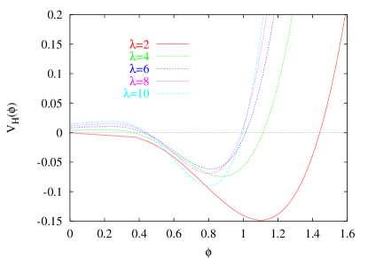
Figure 2: We set $T=1$, and plot the Hartree effective potential as a function of the coupling constant.

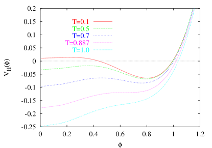
Figure 3: We set $\lambda=7.3$, and plot the Hartree effective potential as a function of temperature.

V Initial Conditions

For the purpose of this study, we will assume that initially (at $t=0$) the system is described by a Gaussian density matrix. Thus initially the field equation and two-point equation is that of the Hartree approximation. The field equation obeys (40), with $G_{0}(x,x^{\prime})$ satisfying:

$$[\,\Box+\chi(t)\,]\,G_{0}(x,x^{\prime})=\delta_{\mathcal{C}}(x,x^{\prime})\>.$$ (45)

We can solve this Green function equation by introducing a set of quantum fields $\phi_{0}(x)$, satisfying canonical commutation relations $[\,\phi_{0}(x),\dot{\phi}_{0}(x^{\prime})\,]=i\,\delta(x-x^{\prime})\>$, and obeying the homogeneous differential equation

$$[\,\Box+\chi(t)\,]\,\phi_{0}(x)=0\>.$$ (46)

In terms of these fields we have

$$G_{0}(x,x^{\prime}) =i\,\langle\,\mathcal{T}_{\mathcal{C}}\{\,\phi_{0}(x)\,\phi_{0}(x^{\prime})\,\}\rangle\>,$$

$$=G_{>}(x,x^{\prime})\,\Theta_{\mathcal{C}}(t,t^{\prime})+G_{<}(x,x^{\prime})\,\Theta_{\mathcal{C}}(t^{\prime},t)\>,$$

$$=\int_{-\infty}^{+\infty}\frac{\mathrm{d}k}{2\pi}\,\tilde{G}_{0}(k;t,t^{\prime})\,e^{ik(x-x^{\prime})}\>.$$ (47)

We next expand these operators in Fourier mode functions

$$\phi_{0}(x)=\int_{-\infty}^{+\infty}\frac{\mathrm{d}k}{2\pi}\,\Bigl{[}\,a_{0\,k}^{\phantom{\dagger}}\,f_{k}^{\phantom{\ast}}(t)\,e^{ikx}+a_{0\,k}^{\dagger}\,f_{k}^{\ast}(t)\,e^{-ikx}\,\Bigr{]}\>,$$ (48)

where the mode functions $f_{k}^{\phantom{\ast}}(t)$ satisfy:

$$[\,\partial_{t}^{2}+\omega_{k}^{2}(t)\,]\,f_{k}(t)=0\>,\qquad\omega_{k}(t)=\sqrt{k^{2}+\chi(t)}\>,$$ (49)

and the Wronskian condition: $f_{k}^{\ast}(t)\,\dot{f}_{k}^{\phantom{\ast}}(t)-\dot{f}_{k}^{\ast}(t)\,f_{k}^{\phantom{\ast}}(t)=-i$. The operators $a_{0\,k}^{\phantom{\dagger}}$ and $a_{0\,k}^{\dagger}$ satisfy the usual commutation relations: $[\,a_{0\,k}^{\phantom{\dagger}},a_{0\,k^{\prime}}^{\dagger}\,]=2\pi\,\delta(k-k^{\prime})$. We will take our initial density matrix such that:

$$\langle\,a_{0\,k}^{\dagger}\,a_{0\,k^{\prime}}^{\phantom{\dagger}}\,\rangle =n_{k}\,2\pi\,\delta(k-k^{\prime})\>, \langle\,a_{0\,k}^{\phantom{\dagger}}\,a_{0\,k^{\prime}}^{\phantom{\dagger}}\,\rangle =0\>,$$

$$\langle\,a_{0\,k}^{\phantom{\dagger}}\,a_{0\,k^{\prime}}^{\dagger}\,\rangle =(n_{k}+1)\,2\pi\,\delta(k-k^{\prime})\>, \langle\,a_{0\,k}^{\dagger}\,a_{0\,k^{\prime}}^{\dagger}\,\rangle =0\>,$$ (50)

where $n_{k}=1/[\,\exp(\beta_{0}\omega_{k}(0))-1\,]$. Here $T_{0}=1/\beta_{0}$ is just a parameter for the initial Gaussian density distribution, and is not the true temperature of the interacting system. In fact, the system will not be in equilibrium at $t=0$, but will arrive at a final temperature $T$ after it has come to equilibrium.

Solutions for the mode functions $f_{k}^{\phantom{\ast}}(t)$ are of the form:

$$f_{k}^{\phantom{\ast}}(t)=\frac{e^{-i\int_{0}^{t}\Omega_{k}(t^{\prime})\mathrm{d}t^{\prime}}}{\sqrt{2\Omega_{k}(t)}}\>,$$ (51)

where $\Omega_{k}(t)$ satisfies the non-linear differential equation,

$$\frac{1}{2}\left(\frac{\ddot{\Omega}_{k}(t)}{\Omega_{k}(t)}\right)-\frac{3}{4}\left(\frac{\dot{\Omega}_{k}(t)}{\Omega_{k}(t)}\right)^{\!2}+\Omega^{2}_{k}(t)=\omega^{2}_{k}(t)\>.$$ (52)

The first order WKB solution for $f_{k}^{\phantom{\ast}}(t)$ is then given by $\Omega_{k}(t)=\omega_{k}(t)$. We take these solutions for our initial conditions, so that at $t=0$,

$$\Omega_{k}(0) =\omega_{k}(0) =\sqrt{k^{2}+\chi(0)}\>,$$

$$\dot{\Omega}_{k}(0) =\dot{\omega}_{k}(0) =\dot{\chi}(0)/2\omega_{k}(0)\>.$$ (53)

This means that

$$f_{k}(0) =1/\sqrt{2\omega_{k}(0)}\>,$$

$$\dot{f}_{k}(0) =-\left[\frac{\dot{\omega}_{k}(0)}{2\omega_{k}(0)}+i\omega_{k}(0)\right]\,f_{k}(0)\>.$$ (54)

We still need to find the value of $\chi_{0}(0)$. This is given by the Hartree self-consistent solutions of:

$$\chi(0)= -\mu^{2}+\frac{3\lambda}{2}\,\phi^{2}(0)+\frac{3\lambda}{2}\,\int_{0}^{+\infty}\frac{\mathrm{d}k}{2\pi}\,\frac{2n_{k}+1}{\sqrt{k^{2}+\chi(0)}}\>,$$

$$= -m^{2}+\frac{3\lambda}{2}\,\phi^{2}(0)$$ (55)

$$+\frac{3\lambda}{2}\,\int_{0}^{\Lambda}\frac{\mathrm{d}k}{2\pi}\,\left[\,\frac{2n_{k}+1}{\sqrt{k^{2}+\chi(0)}}-\frac{1}{\sqrt{k^{2}+m^{2}}}\,\right]\>.$$

Where we have used Eq. (41).

So, for our case, Fourier transforms of the Green functions at $t=0$ are given by:

$$\tilde{G}_{0\,>}(k;t,t^{\prime})/i =f_{k}^{\phantom{\ast}}(t)f_{k}^{\ast}(t^{\prime})\,(n_{k}+1)+f_{k}^{\ast}(t)f_{k}^{\phantom{\ast}}(t^{\prime})\,n_{k}\>,$$

$$\tilde{G}_{0\,<}(k;t,t^{\prime})/i =f_{k}^{\ast}(t)f_{k}^{\phantom{\ast}}(t^{\prime})\,(n_{k}+1)+f_{k}^{\phantom{\ast}}(t)f_{k}^{\ast}(t^{\prime})\,n_{k}\>.$$ (56)

These results, together with Eq. (54), determine the values of $\tilde{G}_{0\,>}(k;t,t^{\prime})$, and all it’s derivatives, at $t=t^{\prime}=0$.

VI Numerical results

We choose initial conditions for the two-point functions as described in the last section. In all our simulations we set the renormalized mass parameter $m$, as defined in Eq. (41), to unity. We have verified numerically that our results are independent of the cut-off parameter $\Lambda$ for values of $\Lambda$ between $3\pi$ and $4\pi$. The numerical procedure for solving the BVA equations is described in detail in Refs. Mihaila and Mihaila (2002); Mihaila and Shaw (2002). The energy is numerically conserved to better than five significant figures for all our simulations. The calculations are carried out entirely in momentum space, and the results are free of artifacts related to the finite volume of a lattice in coordinate space. For a discussion of differences between the continuum and the periodic lattice approach, respectively, we refer the reader to our previous paper, Ref. Mihaila and Dawson (2002).

We start by choosing an initial temperature $T_{0}=0.1$ so as to bring out the quantum nature of the dynamics. The Hartree effective potential for this value of $T_{0}$ is a slowly varying function of the coupling constant, with the minimum value of $\phi$ at large $\lambda$ being between $0.6$ and $1.0$ (see Figs. 2 and 3). Thus we want to choose small initial values of $\phi(0)=0.4$ and take $\pi(0)=\dot{\phi}(0)=0$ so that we start below the height of the barrier. Then we should see $\phi$ moving to the opposite side of the well and then settling down at the potential minimum position. We show the results of this calculation in Figs. 4 and 5 for several values of the coupling constant. We notice that the position of the BVA minimum is located between $0.55$ and $0.60$ instead of the Hartree average value of $0.8$. We also see that the final value of $\chi$ does seem to be linear in $\lambda$ as in the Hartree result. However, the ratio $\chi/(\lambda v^{2})$ is one for the Hartree approximation, but is about $2.4$, with a less than 1% error, for the BVA simulations.

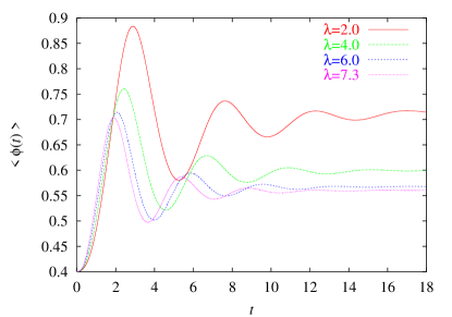
Figure 4: Coupling constant dependence: We set $T_{0}=0.1$, and plot $\langle\phi(t)\rangle$ for various values of $\lambda$.

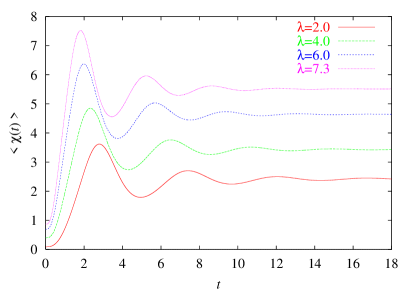
Figure 5: Coupling constant dependence: We set $T_{0}=0.1$, and plot $\langle\chi(t)\rangle$ for various values of $\lambda$.

Next we set $\lambda=7.3$, which is the phenomenological choice for the the linear sigma model, with $\phi(0)=0.4$ and $\pi(0)=\dot{\phi}(0)=0$, and study the dependence of $\langle\phi(t)\rangle$ and $\langle\chi(t)\rangle$ as a function of the initial temperature $T_{0}$. The results are shown in Figs. 6 and 7. We note immediately from Fig. 6 that for small values of $T_{0}$, $\langle\phi(t)\rangle$ equilibrates to non-zero values, but for large values of $T_{0}$, $\langle\phi(t)\rangle$ equilibrates to zero, as expected from the Hartree effective potential. Fig. 7 shows that $\chi(t)$ equilibrates to different values which depend on $T_{0}$.

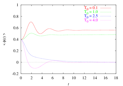
Figure 6: Temperature dependence: We set $\lambda=7.3$, and plot $\langle\phi(t)\rangle$ for various values of $T_{0}$.

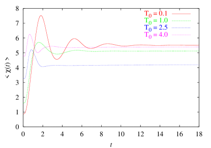
Figure 7: Temperature dependence: We set $\lambda=7.3$, and plot $\langle\chi(t)\rangle$ for various values of $T_{0}$.

Since we have chosen the case $\pi(0)=\dot{\phi}(0)=0$, with $\phi(0)$ just under the barrier height, the transition to the equilibration point is very slow, i.e. equilibration is reached without too many exciting features. It is interesting to give the system a little initial kinetic energy so that structure is introduced in the dynamics but the equilibration value of $\langle\phi(t)\rangle$ remains the same. We illustrate this in Fig. 8.

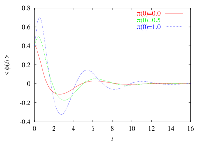
Figure 8: We are increasing the kinetic energy: We set $\lambda=7.3$, $T_{0}=0.1$, and plot $\langle\phi(t)\rangle$ .

The plots of the BVA order parameter in Fig. 6 indicate that for very low values of $T_{0}$, the order parameter $\langle\phi(t)\rangle$ approaches a non-zero constant. For very large values of $T_{0}$, the order parameter goes to zero, as expected. Somewhere between $T_{0}=1.0$ and $T_{0}=2.5$, there seems to be a phase transition. In order to study this in more detail, we have carried out BVA simulations for temperatures between $T_{0}=1.5$ and $T_{0}=2.5$ at $0.1$ intervals. The results for the order parameter and its first derivative are shown in Figs. 9 and 10.

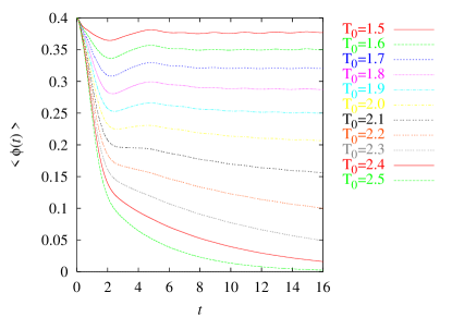
Figure 9: Detailed temperature dependence: We set $\lambda=7.3$, and plot $\langle\phi(t)\rangle$ .

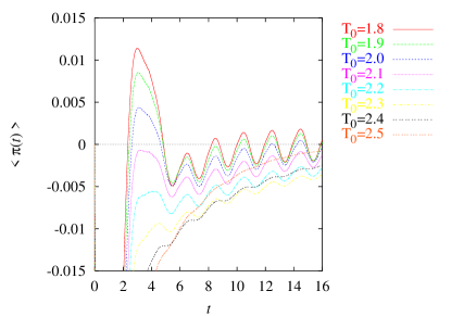
Figure 10: Detailed temperature dependence: We set $\lambda=7.3$, and plot $\langle\dot{\phi}(t)\rangle$ .

The equilibration points for the order parameter in Fig. 9 are at almost equally spaced intervals for $T_{0}<2.4$, and there is no evidence of a jump in the value of the order parameter from a finite value to zero, as would be required by a first order phase transition. The plot of $\langle\dot{\phi}(t)\rangle$, shown in Fig. 10, reveals the complex nature of the dynamics: $\langle\dot{\phi}(t)\rangle$ oscillates and gradually approaches zero, when equilibration occurs. Oscillations around a zero value of $\langle\dot{\phi}(t)\rangle$ suggest the trapping in a potential well, while the wiggles at negative values of $\langle\dot{\phi}(t)\rangle$ may be due to changes in the position of the local minimum of the effective potential as a function of temperature and time. Since the chosen initial conditions do not represent an equilibrium state for the interacting system, the dynamics toward a final state of equilibrium is accompanied by changes in the effective temperature. In other words, the effective potential is not such a good guide to the dynamics. In analyzing these figures, it becomes apparent that a) there is no abrupt change that would support the first-order labeling of the phase transition, and b) there is a qualitative change happening near $T_{0}=2.4$, where the $\langle\dot{\phi}(t)\rangle$ plot begins crossing the lower temperature curves, and the local oscillations in $\langle\dot{\phi}(t)\rangle$ completely disappear. Therefore, we conclude that the phase transition, as calculated using the BVA, is probably not first order.

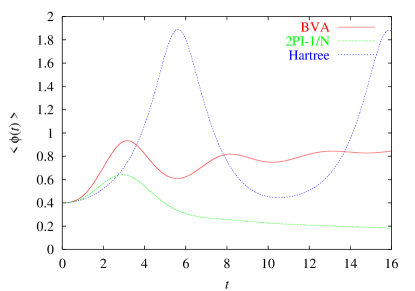
Figure 11: Comparison of various methods: We set $\lambda=1.0$ and $T_{0}=0.1$, and plot $\langle\phi(t)\rangle$.

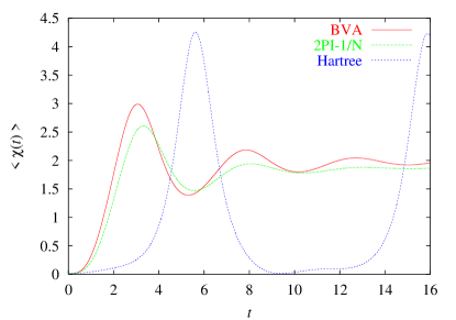
Figure 12: Comparison of various methods: We set $\lambda=1.0$ and $T_{0}=0.1$, and plot $\langle\chi(t)\rangle$.

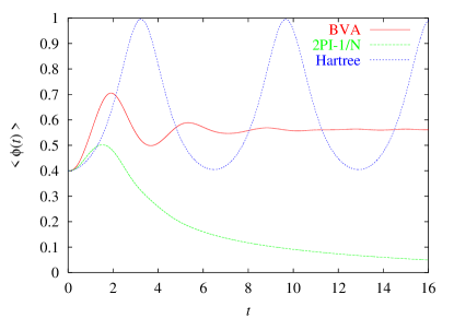
Figure 13: Comparison of various methods: We set $\lambda=7.3$ and $T_{0}=0.1$, and plot $\langle\phi(t)\rangle$.

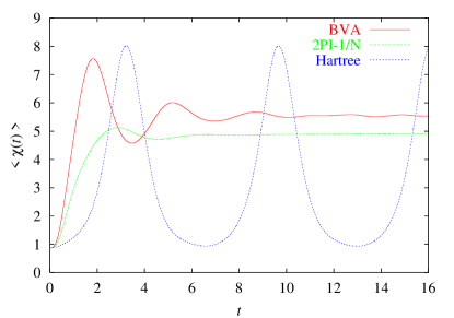
Figure 14: Comparison of various methods: We set $\lambda=7.3$ and $T_{0}=0.1$, and plot $\langle\chi(t)\rangle$.

It is known that this model in two-dimensions has no phase transition at finite temperature Brezin and Zinn-Justin (1976). At zero temperature, there is a second order phase transition Chang (1976); Drell et al. (1977); Banks (1978). Explicit Monte Carlo lattice calculations Amaral et al. (1985, 1986) have shown that indeed $\lambda\phi^{4}$ theory in two-dimensions and at zero temperature is non-trivial at least when the continuum limit is reached from the broken symmetry phase, and that the symmetry is fully restored at high temperature. It is known however that approximate lattice calculations (such as the variational-cumulant expansion method Li and l. Chen (1995, 1997)), which are designed to study scalar $\phi^{4}$ theory in 3+1 dimensions on the lattice, may erroneously indicate the presence of a second-order phase transition at finite temperature in 1+1 dimensions. This is probably due to the fact that the expansion is only carried out to third order. Much in the same way, the Hartree approximation exhibits a first order phase transition with $T_{\text{cr}}\approx 0.878$. When going beyond the Hartree approximation (using the BVA) we still find a phase transition, but the BVA relaxes the order of the phase transition. At very low temperature, we do (apparently) find a non-zero value of the order parameter as $t\rightarrow\infty$, which is the exact result at zero temperature. So we conclude that the BVA at low temperature is seeing effects that might occur in higher dimensions, even though it is not technically correct in 1+1 dimensions.

We next compare three different approximation methods: Hartree, the 2PI-1/N expansion, and BVA. Here we choose a very low initial temperature of $T_{0}=0.1$ in order to emphasize quantum effects in the dynamics. Again, we start with $\langle\phi(0)\rangle=0.4$ and $\langle\dot{\phi}(0)\rangle=0$. We show results for $\lambda=1$ in Figs. 11 and 12 and $\lambda=7.3$ in Figs. 13 and 14. As expected, we find that the Hartree approximation leads to oscillation about the Hartree minimum without equilibration. The BVA results track the Hartree curve, except with damping, and go to a non-zero value as $t\rightarrow\infty$, which is the exact result at zero temperature. The 2PI-1/N expansion goes to a zero value of the order parameter, in agreement with the exact result of no phase transition for finite temperature. Results for $\langle\chi(t)\rangle$ are similar for both approximations, in agreement with expectations based on our experience with the classical limit of these approximations Cooper et al. (2002). The disagreement between 2PI-1/N and BVA is more pronounced at larger values of $\lambda$, as shown in Figs. 13 and 14.

VII Thermalization

The BVA leads to thermalization of the system. In order to have a measure of the semi-static thermodynamic properties of the system, it is reasonable to fit our time-dependent Green functions to those appropriate to a free field with frequency $\omega_{k}(t)$ and Bose-Einstein distribution function $n_{k}(t)$, see also Aarts and Berges (2001). That is, we equate the Fourier transform of the BVA Green functions $\tilde{G}_{k}(t,t)$ and $\partial^{2}\tilde{G}_{k}(t,t^{\prime})/\partial t\,\partial t^{\prime}$ to the corresponding free-field cases:

$$\tilde{G}_{k}(t,t)=[2n_{k}(t)+1]\,\frac{1}{2\omega_{k}(t)}\>,$$ (57)

$$\left.\frac{\partial^{2}\tilde{G}_{k}(t,t^{\prime})}{\partial t\,\partial t^{\prime}}\right|_{t=t^{\prime}}=[2n_{k}(t)+1]\,\frac{\omega_{k}(t)}{2}\>,$$ (58)

where we set

$$n_{k}(t)=\frac{A(t)}{e^{\omega_{k}(t)/T_{\text{eff}}(t)}-1}\>,$$

$$\omega_{k}(t)=\sqrt{k^{2}+m^{2}_{\text{eff}}(t)}\>,$$ (59)

with $m^{2}_{\text{eff}}(t)$ the effective mass and $T_{\text{eff}}(t)$, the effective temperature at time $t$. The factor $A(t)$ comes from a wave function renormalization at each time $t$. So we can determine $n_{k}(t)$ and $\omega_{k}(t)$ from the relations:

$$\omega_{k}(t)=\left[\left.\frac{\partial^{2}G(t,t^{\prime};k)}{\partial t\,\partial t^{\prime}}\right|_{t=t^{\prime}}\ \Big{/}\ G(t,t;k)\right]^{\frac{1}{2}}\>,$$ (60)

$$n_{k}(t)=\frac{1}{2}+\left[\left.\frac{\partial^{2}G(t,t^{\prime};k)}{\partial t\,\partial t^{\prime}}\right|_{t=t^{\prime}}\ G(t,t;k)\right]^{\frac{1}{2}}\>.$$ (61)

¿From (60), we notice that $\omega_{k}$ is a ratio of Green functions, and thus any (finite) wave function renormalization will cancel. However from (61), $n_{k}$ is directly proportional to the Green function, which will have a finite wave function renormalization when restricted to the single particle contribution.

Figure 15: For $\lambda=7.3$ and $T_{0}=2.5$ we plot the time evolution of $\omega_{k}$.

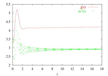
Figure 16: For $\lambda=7.3$ and $T_{0}=2.5$ we compare $m^{2}(t)$ and $\chi(t)$.

First let us concentrate on $\omega_{k}(t)$. We show in Fig. 15 a plot of $\omega_{k}(t)$ as a function of $k$ for various values of $t$, as calculated from Eq. (60), for $\lambda=7.3$ and $T_{0}=2.5$, which is close to the critical temperature. We fit the $\omega_{k}(t)$ data to determine the values of $m^{2}_{\text{eff}}(t)$. These results are compared to the value of $\chi(t)$ in Fig. 16. We see here that self-energy corrections to the effective mass reduce the effective mass to about 25-40% of $\chi(t)$. Further calculations for different initial temperatures allow us to conclude that the correction slowly decreases with increasing initial temperature.

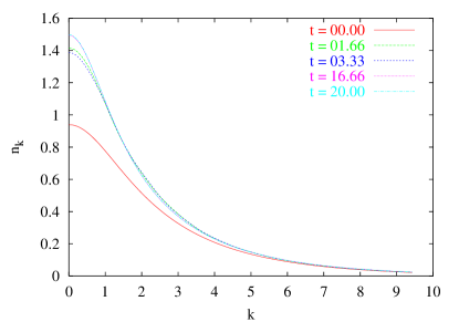
Figure 17: For $\lambda=7.3$ and $T_{0}=2.5$ we plot the time evolution of $n_{k}$, before renormalization.

Now that we have the effective $\omega_{k}$ we can find out if the particle number density $n_{k}(t)$ has the simple Bose-Einstein form given in Eq. (59). We use a nonlinear fitting procedure to obtain the parameters $T_{\text{eff}}(t)$ and $A(t)$ from the data generated by Eq. (61). The results are shown in Fig. 17 for $\lambda=7.3$ and $T_{0}=2.5$. In Fig. 19 we show the renormalized densities, given by $n_{\text{ren}\,k}(t)=n_{k}(t)/A(t)$. Notice that $n_{k}(t)$ is very similar to a Bose-Einstein distribution which starts out at a temperature of $T_{\text{eff}}=T_{0}$, increases in amplitude due to a temperature increase, then falls back to a lower temperature, but larger mass.

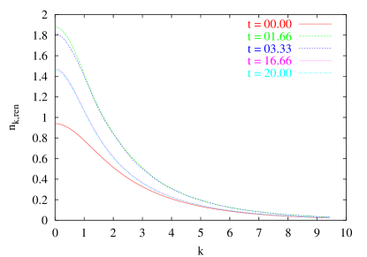
Figure 18: For $\lambda=7.3$ and $T_{0}=2.5$ we plot the time evolution of $n_{k,\text{ren}}$, after renormalization.

Figure 19: For $\lambda=7.3$ and $T_{0}=2.5$ we plot the time evolution of the temperature $T_{k,\text{ren}}(t)$.

In Fig. 19 we show the effective temperature profile, $T_{k,\text{ren}}(t)$ inferred from $n_{k,\text{ren}}(t)$

$$T_{\text{ren}\,k}(t)=\omega_{k}(t)\,/\,\ln\bigl{[}\,(n_{\text{ren}\,k}(t)+1)/(n_{\text{ren}\,k}(t))\,\bigr{]}\>.$$ (62)

We notice that at short times, $T_{\text{ren}\,k}(t)$ has to readjust to the effects of the non-Gaussian corrections, but then it settles down to a new temperature which is relatively independent of the momentum $k$. We also notice that we do have quite a bit of particle production: after an initial spike, the particle density number relaxes to an equilibrium value.

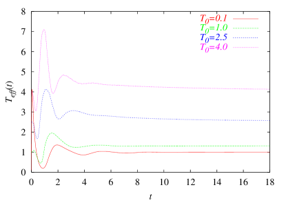
Figure 20: For $\lambda=7.3$ we plot the time evolution of $T_{\text{eff}}(t)$ for various initial temperatures $T_{0}$.

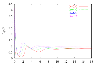
Figure 21: For $T_{0}=0.1$ we plot the time evolution of $T_{\text{eff}}(t)$ for various values of the coupling constant $\lambda$.

In Fig. 20 we show the dependence of $T_{\text{eff}}$ on the initial temperature $T_{0}$, for fixed $\lambda=7.3$, and in Fig. 21, the dependence of $T_{\text{eff}}$ on the coupling constant $\lambda$ for fixed $T_{0}=0.1$.

VIII Conclusions

In conclusion, we have shown that the BVA indeed leads to equilibration of the one- and two-point functions and thus remedies this deficiency of the Hartree approximation. The nature of the phase transition changes from first to second order when going from Hartree to BVA which is the correct behavior (as a function of coupling constant) at zero temperature but is incorrect at higher temperature. However, such a phase transition at finite temperature is expected in the 3+1 dimensional case that we are interested in modeling in the future. The 2PI-1/N approximation does not see this phase transition (which is not present in the exact theory) and does not track the average of the Hartree result. In higher dimensions, one expects the Hartree result for the order parameter to be correct on the average but not have the property of equilibrating. So deciding which approximation is more physical will have to wait for a 3+1 dimensional simulation to see if both approximations show a phase transition.

In the classical regime, where we could do an exact Monte Carlo calculation, we found that the BVA works better than the 2PI-1/N expansion in capturing the dynamics of $\langle\phi(t)\rangle$, but that the difference was not very great. In the quantum domain, however, these two approximations diverge at low temperature with the strength of the coupling constant, and the 2PI-1/N approximation no longer tracks the average of the results of the Hartree approximation. Since we do not have exact calculations in the quantum regime, we cannot make any strong conclusions about this divergence.

It is interesting to note that technical issues related to the nature of the phase transitions in 1+1 dimensions are not uncommon. There is a previous example of just this very type of reasoning being successful. In trying to understand the QCD chiral phase transition at finite chemical potential and temperature, it was important to have a model where the phase transition mimicked what is known in 3+1 dimensions. Such a model was a four-fermi model (the Gross-Neveu model) in 1+1 dimensions in leading order in large-N, which had a similar phase structure to two-flavor QCD. This model was then used as a testing ground for studying the effect of first and second order phase transitions, with a critical point, and showed some qualitative differences between the two types of transitions (see Ref. Chodos et al. (2001)). Once again, the exact 1+1 dimensional model does not have a phase transition. But this warmup problem then allowed us to go to 2+1 dimensionsCooper and Savage (2002), where it is known that the leading order large-N approximation and the exact theory have similar phase diagrams, as verified by lattice simulations in 2+1 dimensions Hands et al. (2001). We submit that this is the way these 1+1 dimensional results should be understood: as a model having certain properties when treated in this approximation and as a testing ground for codes which will then be generalized to higher dimensions where it is expected the approximation will correspond to the known behavior. The main purpose of the quantum simulations we present here is to get experience in getting codes working in lower dimensions that qualitatively do what we expect to see in 3+1 dimensions.

As a result of the simulations presented here, we are confident that we can now study the chiral phase transition in 3+1 dimensions in the linear sigma model and describe the competition between the expansion of the plasma and the equilibration tendencies. This will allow us to see whether some of the phenomena present in Hartree (and/or large-N) approximation, such as production of disoriented chiral condensates and distortion of pion and dilepton spectra, are still present in spite of the forces that lead to thermalization.