hep-ph/0209048
Ward identity and electrical conductivity in hot QED

Abstract

We study the Ward identity for the effective photon-electron vertex summing the ladder diagrams contributing to the electrical conductivity in hot QED at leading logarithmic order. It is shown that the Ward identity requires the inclusion of a new diagram in the integral equation for the vertex that has not been considered before. The real part of this diagram is subleading and therefore the final expressions for the electrical conductivity at leading logarithmic order are not affected.

1 Introduction

Transport coefficients in quantum field theories at finite temperature have received an increasing amount of attention over the last few years, not only because of their potential relevance in some physical environments, such as heavy-ion collisions and the early universe, but also because, from a theoretical point of view, their calculation turns out to be highly nontrivial. A perturbative analysis can be used when the temperature is sufficiently high and the theory is weakly coupled. However, the computation of transport coefficients in hot gauge theories within the framework of thermal field theory remains a difficult task due to the necessity of summing an infinite number of Feynman diagrams, so-called ladder diagrams [1]. This has favoured the use of effective descriptions such as transport theory [2, 3, 4]. Another alternative is the use of lattice field theory [5], which allows one in principle to obtain transport coefficients at temperatures where a perturbative analysis (either with field or transport theory) is not valid. This approach has not been completely developed and presents its own difficulties [6].

It is within the kinetic approach that it was first realized that screening processes in the plasma at the scale of the Debye mass are enough to render results finite [2]. The first complete calculation of transport coefficients in hot gauge theories at leading logarithmic order appeared only recently [4], also using kinetic theory. For a scalar theory the ladder diagrams have been summed explicitly by Jeon [7] using a Bethe-Salpeter equation for an effective vertex and the leading-order results for the shear and bulk viscosities have been obtained. The conclusions of his diagrammatic analysis have been confirmed in Refs. [8]. Furthermore, Jeon and Yaffe [9] showed the equivalence between the diagrammatic and the kinetic approach: to leading order the linearized Boltzmann equation for the distribution function and the Bethe-Salpeter equation for the effective vertex yield equivalent results. For QCD, a simplified ladder summation [10] reproduces the result for the color conductivity at leading logarithmic order [11].

Only very recently a simple and economical way of summing the ladder series via a Bethe-Salpeter equation in the imaginary-time formalism has been presented by Valle Basagoiti [12], for both scalar and (non)abelian gauge theories. To leading logarithmic order, the integral equations obtained in Ref. [12] are identical to those found previously in the kinetic approach [4]. However, for gauge theories the integral equations for the effective vertices used in Ref. [12] are not consistent with the Ward identities. In the case of the electrical conductivity in QED, which we will consider in this paper, this can be understood as follows. As usual, the photon-electron vertex and the fermion propagator are related via the Ward identity. A typical ladder diagram contributing to the electrical conductivity at leading logarithmic order is shown in Fig. 1. Propagators for the nearly on-shell fermions on the side rails with hard momentum ($p\equiv|{\mathbf{p}}|\sim T$, with $T$ the temperature) have to include the fermionic thermal width, such that singularities due to so-called pinching poles are regulated. This thermal width receives contributions from processes involving both a soft ($p\sim eT$) photon and a soft fermion. Ladder diagrams as the one shown in Fig. 1 can be summed by introducing an effective photon-electron vertex involving a soft photon rung [12].

Figure 1: Typical ladder diagram contributing to the electrical conductivity. The side rails are hard, nearly on-shell fermions and the rungs are soft photons.

One expects that the Ward identity relates the contribution to the thermal width from soft photons to the vertex with a soft photon rung. However, the contribution to the thermal width from soft fermions, appearing at order $e^{4}T\ln(1/e)$, has no counterpart in the equation for the vertex function presented in Ref. [12]. Therefore, the Ward identity is not fulfilled and the equation for the effective vertex given in Ref. [12] cannot be complete. We show in this paper that in order to satisfy the Ward identity a new diagram involving soft fermions has to be included, so that the integral equation is the one depicted in Fig. 2. As far as we know, this diagram has not been discussed before.

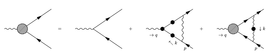
$\Gamma^{\mu}$                               $\gamma^{\mu}$                              $\Gamma_{\rm HTL}^{\mu}$                             $\Gamma_{\rm ladder}^{\mu}$

Figure 2: Integral equation for the effective photon-electron vertex function $\Gamma^{\mu}$. The second diagram on the right-hand-side with a hard photon and HTL vertex and fermion propagators is new and is required to fulfill the Ward identity.

Concerning the electrical conductivity, however, only the real part of the effective photon-electron vertex is required. It turns out that the real part of the new diagram is parametrically suppressed with respect to the tree-level vertex. Therefore we find that the presence of the vertex correction involving soft fermions does not affect the final result for the electrical conductivity at leading logarithmic order.

The paper is organized as follows. In Sec. 2 we review the derivation of the electrical conductivity in terms of a particular analytic continuation of the effective vertex of Ref. [12]. The complete thermal width of order $e^{4}T\ln(1/e)$ for an on-shell electron with hard momentum is computed in Sec. 3. In Sec. 4 we show the consistency of the modified vertex equation with the Ward identity. In Sec. 5 we show that the new integral equation leads to the same leading-log differential equation as in Refs. [4, 12] for that piece of the effective vertex relevant for the electrical conductivity. Conclusions are presented in Sec. 6. We have summarized convenient sum rules in Appendix A. The calculation of the new diagram is detailed in Appendix B.

2 Electrical conductivity

The Kubo formula for the electrical conductivity in QED is

$$\sigma=\frac{1}{6}\,\frac{\partial}{\partial q^{0}}\rho(q^{0},{\mathbf{0}})\Big{|}_{q^{0}=0},$$ (1)

where $\rho$ is the spectral density associated with the spatial part of the retarded polarization tensor

$$\rho(q^{0},{\mathbf{q}})=2{\mathrm{Im}}\,\Pi^{ii}_{R}(q^{0},{\mathbf{q}}),\hskip 28.45274pt\Pi^{ii}_{R}(x-y)=i\theta(x^{0}-y^{0})\langle[j^{i}(x),j^{i}(y)]\rangle,$$ (2)

with $j^{i}(x)=\bar{\psi}(x)\gamma^{i}\psi(x)$ the electromagnetic current. The retarded correlator can be obtained from the Euclidean one by analytical continuation,

$$\Pi^{ii}_{R}(q^{0},{\mathbf{q}})=\Pi^{ii}_{E}(i\omega_{q}\to q^{0}+i0^{+},{\mathbf{q}}),$$ (3)

with $\omega_{q}=2\pi nT$ ($n\in\mathbb{Z}$) the Matsubara frequency. The relevance of ladder diagrams for the conductivity can be understood as follows. We start with the simple one-loop expression: since in the Kubo formula (1) the correlator appears with vanishing external momentum, the fermionic propagators in the one-loop expression share almost the same momentum and so-called pinching poles are present. They cause the one-loop contribution to diverge unless the thermal width is present in the electron propagators [1]. Because the dominant contribution arises when the electrons are on-shell and carry hard momentum, the width is included by replacing the Dirac delta functions of the free single-particle spectral densities with Lorentzian spectral functions

$$\rho^{\rm{free}}_{\pm}(\omega,{\mathbf{p}})=2\pi\delta(\omega\mp p)\longrightarrow\rho_{\pm}(\omega,{\mathbf{p}})=\frac{\Gamma_{{\mathbf{p}}}}{(\omega\mp p)^{2}+(\Gamma_{{\mathbf{p}}}/2)^{2}},$$ (4)

where $\Gamma_{{\mathbf{p}}}$ is the thermal width of a fermion with hard on-shell momentum. These positive- and negative-energy spectral densities are related to the electron propagator as

$$S(p^{0},{\mathbf{p}})=\Delta_{+}(p^{0},{\mathbf{p}})h_{+}(\hat{{\mathbf{p}}})+\Delta_{-}(p^{0},{\mathbf{p}})h_{-}(\hat{{\mathbf{p}}}),\;\;\;\;\;\;\;\Delta_{\pm}(p^{0},{\mathbf{p}})=-\int\frac{d\omega}{2\pi}\frac{\rho_{\pm}(\omega,{\mathbf{p}})}{p^{0}-\omega},$$ (5)

with

$$h_{+}(\hat{{\mathbf{p}}})=\frac{1}{2}\left(\gamma^{0}-\boldsymbol{\gamma}\cdot\hat{{\mathbf{p}}}\right)=\sum_{\lambda}u_{\lambda}(\hat{{\mathbf{p}}})\bar{u}_{\lambda}(\hat{{\mathbf{p}}}),\;\;\;\;\;\;\;h_{-}(\hat{{\mathbf{p}}})=\frac{1}{2}\left(\gamma^{0}+\boldsymbol{\gamma}\cdot\hat{{\mathbf{p}}}\right)=\sum_{\lambda}v_{\lambda}(\hat{{\mathbf{p}}})\bar{v}_{\lambda}(\hat{{\mathbf{p}}}),$$ (6)

where $u_{\lambda}$ ($v_{\lambda}$) are spinors for the electron (positron) in a simultaneous chirality-helicity base ($\lambda=\pm$ indicates the helicity, $\hat{{\mathbf{p}}}={\mathbf{p}}/p$). Similarly we write the self-energy as

$$\Sigma(p^{0},{\mathbf{p}})=\Sigma_{-}(p^{0},{\mathbf{p}})h_{+}(\hat{{\mathbf{p}}})+\Sigma_{+}(p^{0},{\mathbf{p}})h_{-}(\hat{{\mathbf{p}}}).$$ (7)

The use of Lorentzian spectral densities leads to fermionic propagators

$$\Delta_{\pm}(z,{\mathbf{p}})=\frac{-1}{z\mp p-\Sigma_{\pm}(z,{\mathbf{p}})},\hskip 28.45274pt\Sigma_{\pm}(z,{\mathbf{p}})=-i\mbox{sgn}\!\left[{\mathrm{Im}}(z)\right]\frac{\Gamma_{{\mathbf{p}}}}{2}.$$ (8)

This propagator has a cut on the real axis due to the discontinuity of the sign function. In particular, the retarded and advanced propagators and self-energies for hard on-shell fermions are

$$\Delta^{R}_{\pm}(p^{0},{\mathbf{p}})= \frac{-1}{p^{0}\mp p+i\Gamma_{{\mathbf{p}}}/2}=\left[\Delta^{A}_{\pm}(p^{0},{\mathbf{p}})\right]^{*},$$ (9)

$$\Sigma_{\pm}^{R}(p^{0},{\mathbf{p}})= -i\Gamma_{{\mathbf{p}}}/2=\left[\Sigma_{\pm}^{A}(p^{0},{\mathbf{p}})\right]^{*},$$ (10)

when $p^{0}\simeq\pm p$. The presence of the width regulates the pinching-pole divergence in the one-loop expression, which now behaves as $1/\Gamma_{{\mathbf{p}}}$. However, the immediate consequence is the need to sum all ladders diagrams with soft photon rungs, like the one depicted in Fig. 1. Since each new rung introduces a pair of propagators with pinching poles and the width scales (naively) as $e^{2}$, the powers of the coupling constant introduced by the rung are compensated for by the factor $1/\Gamma_{{\mathbf{p}}}$ from the nearly-pinching poles. As a result it is necessary to sum all contributions from uncrossed ladders.

These diagrams can be summed with a Bethe-Salpeter equation for an effective vertex $\Gamma^{\mu}$. In Ref. [12] such an equation was written and it was shown that the spatial part of the integral equation, relevant for the transport coefficient, reduces to leading logarithmic accuracy to a differential equation equivalent to the one obtained previously in Ref. [4] using kinetic theory. As discussed in the Introduction, the equation for the vertex presented in Ref. [12] does not satisfy the Ward identity and can therefore not be complete. In order for the Ward identity to be fulfilled a new diagram has to be included such that the integral equation is the one depicted in Fig. 2.

The Euclidean correlator summing all the ladder diagrams is then given by

$$\Pi_{E}^{ii}(Q)=e^{2}\mbox{$\sum$}\int_{P}{\mathrm{tr}}\,\gamma^{i}S(P+Q)\Gamma^{i}(P+Q,P)S(P),$$ (11)

with $Q=(i\omega_{q},{\mathbf{0}})$. We now follow Ref. [12] to express the electrical conductivity in terms of a particular analytic continuation of the effective vertex. After doing the sum over Matsubara frequencies, only products of retarded and advanced fermion propagators $S^{R}(p^{0}+q^{0},{\mathbf{p}})S^{A}(p^{0},{\mathbf{p}})$ must be retained because only these can have pinching poles. Furthermore, since $q^{0}$ goes to zero, it cannot change the mass shell condition of the electrons on the side rails with hard momentum. Thus pinching poles arise only from the products $\Delta_{\pm}^{R}(p^{0}+q^{0},{\mathbf{p}})\Delta_{\pm}^{A}(p^{0},{\mathbf{p}})$ and we find

$$\Pi_{R}^{ii}(q^{0},{\mathbf{0}})=2ie^{2}\int_{{\mathbf{p}},\omega}\left[n_{F}(\omega+q^{0})-n_{F}(\omega)\right]\bigg{[}\Delta^{R}_{+}(\omega+q^{0},{\mathbf{p}})\Delta^{A}_{+}(\omega,{\mathbf{p}})\hat{p}^{i}D_{+}^{i}(\omega+q^{0},\omega;{\mathbf{p}})$$

$$-\Delta^{R}_{-}(\omega+q^{0},{\mathbf{p}})\Delta^{A}_{-}(\omega,{\mathbf{p}})\hat{p}^{i}D_{-}^{i}(\omega+q^{0},\omega;{\mathbf{p}})\bigg{]},$$ (12)

where $n_{F}(\omega)=1/[\exp(\omega/T)+1]$ is the Fermi distribution, and

$$\int_{{\mathbf{p}},\omega}=\int\frac{d^{3}p}{(2\pi)^{3}}\int\frac{d\omega}{2\pi}.$$ (13)

Here we used

$$h_{\pm}(\hat{{\mathbf{p}}})\gamma^{i}h_{\pm}(\hat{{\mathbf{p}}})=\pm\hat{p}^{i}h_{\pm}(\hat{{\mathbf{p}}}),$$ (14)

and defined

$$D^{\mu}_{+}(\omega+q^{0},\omega;{\mathbf{p}})\equiv \bar{u}_{\lambda}(\hat{{\mathbf{p}}})\Gamma^{\mu}(\omega+q^{0}+i0^{+},\omega-i0^{+};{\mathbf{p}})u_{\lambda}(\hat{{\mathbf{p}}}),$$ (15)

$$D^{\mu}_{-}(\omega+q^{0},\omega;{\mathbf{p}})\equiv \bar{v}_{\lambda}(\hat{{\mathbf{p}}})\Gamma^{\mu}(\omega+q^{0}+i0^{+},\omega-i0^{+};{\mathbf{p}})v_{\lambda}(\hat{{\mathbf{p}}}).$$ (16)

Both helicities give the same result such that the sum over helicities yields a trivial factor 2 in Eq. (2). Note that out of the many vertex functions with real energy arguments [13] only one particular analytical continuation appears. Now, in the limit $q^{0}\to 0$ and in the limit of narrow width (weak coupling), the pair of propagators goes to its pinching-pole limit,

$$\lim_{q^{0}\to 0}\Delta^{R}_{\pm}(\omega+q^{0},{\mathbf{p}})\Delta^{A}_{\pm}(\omega,{\mathbf{p}})=\frac{1}{(\omega\mp p)^{2}+(\Gamma_{{\mathbf{p}}}/2)^{2}}\longrightarrow\frac{2\pi}{\Gamma_{{\mathbf{p}}}}\delta(\omega\mp p),$$ (17)

forcing the on-shell condition $\omega=\pm p$. Since in the pinching-pole limit the product of propagators (17) is real and only the imaginary part of $\Pi_{R}^{ii}(q^{0},{\mathbf{0}})$ is needed for the electrical conductivity, only the real part of the effective vertex contributes. Therefore we define

$${\cal D}^{i}_{\pm}({\mathbf{p}})\equiv{\mathrm{Re}}\,D^{i}_{\pm}(\pm p+q^{0},\pm p;{\mathbf{p}})\Big{|}_{q^{0}=0}.$$ (18)

Finally, since due to rotational invariance ${\cal D}^{i}_{\pm}({\mathbf{p}})=\hat{p}^{i}\,{\cal D}_{\pm}(p)$ and due to $CP$ invariance ${\cal D}_{+}(p)=-{\cal D}_{-}(p)\equiv{\cal D}(p)$, the electrical conductivity is given by

$$\sigma=-\frac{4e^{2}}{3}\int_{{\mathbf{p}}}n_{F}^{\prime}(p)\frac{{\cal D}(p)}{\Gamma_{{\mathbf{p}}}}.$$ (19)

This expression can be easily compared with the result from kinetic theory [4]. The factor 4 reflects that both electrons and positrons with either helicity contribute in the same way.

3 Thermal Width

The electrical conductivity depends on the thermal width $\Gamma_{{\mathbf{p}}}$ of a hard on-shell fermion, which screens the pinching-pole singularity and naturally sets an inverse time scale in the system. Kinetic theory calculations [2, 4] show that the relevant inverse relaxation time for the electrical conductivity is $1/\tau\sim e^{4}T\ln(T/m_{D})\sim e^{4}T\ln(1/e)$, coming from large angle scattering between the hard nearly on-shell fermions in the plasma as well as from scattering processes that change the type of excitation. The thermal width, on the other hand, is dominated by scattering processes in which the fermions exchange a soft quasistatic transverse gauge boson (the leading term is in fact logarithmically divergent, reflecting that in QED the thermal width is ill-defined) [1, 14]. This dominant contribution should therefore not be relevant for the calculation of the electrical conductivity to leading logarithmic order. This is indeed what is found in Refs. [1, 12] and will be confirmed in Section 5. The thermal width, however, receives subleading contributions from scattering regimes different than the previous one. A contribution of order $e^{4}T\ln(1/e)$ arises from the one-loop diagram with a soft fermion (see the second diagram in Fig. 3 below) and has been computed in Ref. [12]. This contribution corresponds to Compton scattering and pair annihilation/creation processes, as can be seen by cutting the diagram, which are mediated by a soft fermion screened at the scale of the Debye mass. As is shown in this section, there is also a contribution to the thermal width of order $e^{4}T\ln(1/e)$ from the one-loop diagram with a soft photon (see the first diagram in Fig. 3). This part arises from scatterings where the electrons exchange a soft photon screened at the scale of the Debye mass.

In order to verify the Ward identity up to a given order in the coupling constant, all processes that contribute up to that order have to be included (in particular, not just those processes that contribute to transport). Therefore, we compute in this section the complete contribution to the thermal width to order $e^{4}T\ln(1/e)$. In Sec. 5 we show how the scale $e^{4}T\ln(1/e)$ actually arises in the field theory calculation of the conductivity, from both soft photon and soft fermion mediated scattering processes. It turns out that only the soft fermion contribution to the thermal width appears explicitly. The processes in which a soft photon, screened at the scale of the Debye mass, is exchanged contribute not through the thermal width but in an indirect way, through the rungs in the ladder diagrams.

The thermal width of an on-shell electron is given by

$$\Gamma_{{\mathbf{p}}}=-2{\mathrm{Im}}\,\Sigma^{R}_{+}(p^{0}=p,{\mathbf{p}}).$$ (20)

The one-loop fermion self-energy reads

$$\Sigma(P)=-e^{2}\mbox{$\sum$}\int_{K}\gamma^{\nu}S(P+K)\gamma^{\mu}D_{\mu\nu}(K).$$ (21)

The Matsubara sum is easily performed using spectral representations. For the photon we work in the Coulomb gauge and the photon propagator reads

$$D_{\mu\nu}(p^{0},{\mathbf{p}})=-\frac{1}{{\mathbf{p}}^{2}}P^{L}_{\mu\nu}-\int_{-\infty}^{\infty}\frac{d\omega}{2\pi}\,\frac{\rho_{\mu\nu}(\omega,{\mathbf{p}})}{p^{0}-\omega},$$ (22)

with

$$\rho_{\mu\nu}(\omega,{\mathbf{p}})=\rho_{T}(\omega,{\mathbf{p}})P^{T}_{\mu\nu}(\hat{{\mathbf{p}}})+\rho_{L}(\omega,{\mathbf{p}})P^{L}_{\mu\nu},$$ (23)

and $P^{T}_{ij}(\hat{{\mathbf{p}}})=\delta_{ij}-\hat{p}_{i}\hat{p}_{j}$, $P^{T}_{0\nu}={\cal P}^{T}_{\mu 0}=0$ and $P^{L}_{\mu\nu}=\delta_{\mu 0}\delta_{\nu 0}$. We find for the imaginary part of the retarded on-shell self-energy,

$${\mathrm{Im}}\,\Sigma^{R}(p,{\mathbf{p}})=-\frac{e^{2}}{2}\int_{{\mathbf{k}},\omega}\left[n_{B}(\omega)+n_{F}(p+\omega)\right]\gamma^{\nu}\rho_{F}(p+\omega,{\mathbf{r}})\gamma^{\mu}\rho_{\mu\nu}(\omega,{\mathbf{k}}),$$ (24)

with ${\mathbf{r}}={\mathbf{p}}+{\mathbf{k}}$, $n_{B}(\omega)=1/[\exp(\omega/T)-1]$ is the Bose distribution, and

$$\rho_{F}(\omega,{\mathbf{k}})=\rho_{+}(\omega,{\mathbf{k}})h_{+}(\hat{{\mathbf{k}}})+\rho_{-}(\omega,{\mathbf{k}})h_{-}(\hat{{\mathbf{k}}}).$$ (25)

With the help of the following useful relations,

$$h_{\pm}(\hat{{\mathbf{p}}})h_{\pm}(\hat{{\mathbf{p}}})=0,\;\;\;\;\;\;\;\;\;\;\;\;\;\;h_{\pm}(\hat{{\mathbf{p}}})h_{\mp}(\hat{{\mathbf{p}}})=\gamma^{0}h_{\mp}(\hat{{\mathbf{p}}})=h_{\pm}(\hat{{\mathbf{p}}})\gamma^{0},$$

$$h_{\pm}(\hat{{\mathbf{p}}})\gamma^{0}h_{\mp}(\hat{{\mathbf{p}}})=0,\;\;\;\;\;\;\;\;\;\;\;h_{\pm}(\hat{{\mathbf{p}}})\gamma^{i}h_{\mp}(\hat{{\mathbf{p}}})=(\pm\hat{p}^{i}-\gamma^{i}\gamma^{0})h_{\mp}(\hat{{\mathbf{p}}}),$$ (26)

$$h_{\pm}(\hat{{\mathbf{p}}})\gamma^{0}h_{\pm}(\hat{{\mathbf{p}}})=h_{\pm}(\hat{{\mathbf{p}}}),$$

and

$$\gamma^{\mu}h_{\pm}(\hat{{\mathbf{p}}})\gamma^{\nu}P^{L}_{\mu\nu}=h_{\mp}(\hat{{\mathbf{p}}}),\;\;\;\;\;\;\;\;\;\gamma^{\mu}h_{\pm}(\hat{{\mathbf{p}}})\gamma^{\nu}P^{T}_{\mu\nu}(\hat{{\mathbf{r}}})=\gamma^{0}\mp\hat{{\mathbf{p}}}\cdot\hat{{\mathbf{r}}}\,\boldsymbol{\gamma}\cdot\hat{{\mathbf{r}}},$$ (27)

the (exact) result for the one-loop width is

$$\Gamma_{{\mathbf{p}}}= e^{2}\int_{{\mathbf{k}},\omega}\left[n_{F}(p+\omega)+n_{B}(\omega)\right]$$ (28)

$$\times\left(\,\rho_{T}(\omega,{\mathbf{k}})\left[\rho_{+}(p+\omega,{\mathbf{r}})(1-\hat{{\mathbf{p}}}\cdot\hat{{\mathbf{k}}}\,\hat{{\mathbf{k}}}\cdot\hat{{\mathbf{r}}})+\rho_{-}(p+\omega,{\mathbf{r}})(1+\hat{{\mathbf{p}}}\cdot\hat{{\mathbf{k}}}\,\hat{{\mathbf{k}}}\cdot\hat{{\mathbf{r}}})\right]\right.$$

$$\left.+\frac{1}{2}\rho_{L}(\omega,{\mathbf{k}})\left[\rho_{+}(p+\omega,{\mathbf{r}})(1+\hat{{\mathbf{p}}}\cdot\hat{{\mathbf{r}}})+\rho_{-}(p+\omega,{\mathbf{r}})(1-\hat{{\mathbf{p}}}\cdot\hat{{\mathbf{r}}})\right]\right).$$

(sp)                                         (sf)

Figure 3: Contributions to the thermal width of a hard on-shell fermion with a soft photon (sp) and a soft fermion (sf).

There are two contributions of order $e^{4}T\ln(1/e)$, arising when either the photon or the fermion carries soft momentum, $\Gamma_{\mathbf{p}}=\Gamma_{\mathbf{p}}^{\rm(sp)}+\Gamma_{\mathbf{p}}^{\rm(sf)}$ (see Fig. 3). We first specialize to the case that the photon is soft, $k\ll p$. In this case the momentum of the fermion inside the loop is hard and its spectral density can be taken as the free one, $\rho_{\pm}^{\rm free}(\omega,{\mathbf{p}})=2\pi\delta(\omega\mp p)$. Since we consider $p^{0}=p$, $\rho_{-}$ does not contribute and we have

$$\Gamma_{{\mathbf{p}}}^{\rm(sp)}= e^{2}\int_{{\mathbf{k}},\omega}\left[n_{F}(p+\omega)+n_{B}(\omega)\right]\rho_{+}^{\rm free}(p+\omega,{\mathbf{r}})$$ (29)

$$\times\left[{}^{\ast}\!\rho_{T}(\omega,{\mathbf{k}})(1-\hat{{\mathbf{p}}}\cdot\hat{{\mathbf{k}}}\,\hat{{\mathbf{k}}}\cdot\hat{{\mathbf{r}}})+\frac{1}{2}{}^{\ast}\!\rho_{L}(\omega,{\mathbf{k}})(1+\hat{{\mathbf{p}}}\cdot\hat{{\mathbf{r}}})\right].$$

The angular integration can be performed with the fermionic spectral function,

$$\rho_{+}^{\rm free}(p+\omega,{\mathbf{r}})=2\pi\delta(p+\omega-r)\to 2\pi\frac{p+\omega}{pk}\,\delta(z-z_{0})\theta(k^{2}-\omega^{2}),\;\;\;z_{0}=\frac{\omega}{k}+\frac{\omega^{2}-k^{2}}{2pk},$$ (30)

where $z$ is the cosine of the angle between ${\mathbf{k}}$ and ${\mathbf{p}}$. We find for the contribution with the soft photon

$$\Gamma^{\rm{(sp)}}_{{\mathbf{p}}}= \frac{\alpha}{2p^{2}}\int_{\Lambda_{min}}^{\Lambda_{max}}\!\!\!\!dk\,k\int_{-k}^{k}\frac{d\omega}{2\pi}\,\left[n_{F}(p+\omega)+n_{B}(\omega)\right]$$ (31)

$$\times\left({}^{\ast}\!\rho_{T}(\omega,k)\frac{k^{2}-\omega^{2}}{k^{2}}\left[(\omega+2p)^{2}+k^{2}\right]+{}^{\ast}\!\rho_{L}(\omega,k)\left[(\omega+2p)^{2}-k^{2}\right]\right),$$

with $\alpha=e^{2}/4\pi$. The integral over the momentum $k$ has been restricted between $\Lambda_{min}$, a lower cutoff to avoid the logarithmic singular behaviour, and $\Lambda_{max}$ (with $eT\ll\Lambda_{max}\ll T$ [15]), so that the approximation of soft photon momentum is valid. In order to find contributions up to $e^{4}T\ln(1/e)$, we define $x=\omega/k$ and expand in powers of $k/p$,

$$\Gamma_{\mathbf{p}}^{\rm(sp)}=2\alpha T\int_{\Lambda_{min}}^{\Lambda_{max}}\!\!\!\!dk\,k \int_{-k}^{k}\frac{d\omega}{2\pi}\,\frac{1}{\omega}\left[{}^{\ast}\!\rho_{T}(\omega,k)\left(V_{T}^{(0)}(x)+V_{T}^{(1)}(x)\frac{k}{p}+V_{T}^{(2)}(x)\frac{k^{2}}{2p^{2}}+\ldots\right)\right.$$ (32)

$$\left.+\,{}^{\ast}\!\rho_{L}(\omega,k)\left(V_{L}^{(0)}(x)+V_{L}^{(1)}(x)\frac{k}{p}+V_{L}^{(2)}(x)\frac{k^{2}}{2p^{2}}+\ldots\right)\right],$$

with

$$V_{L}^{(0)}(x)= 1,\hskip 150.79968ptV_{T}^{(0)}(x)=1-x^{2},$$ (33)

$$V_{L}^{(1)}(x)= \frac{1}{2}x(2-\beta p\,[1-2n_{F}(p)]),\;\;\;\;\;\;\;\;\;\;\,V_{T}^{(1)}(x)=(1-x^{2})V_{L}^{(1)}(x),$$ (34)

$$V_{L}^{(2)}(x)= -\frac{1}{2}(1-x^{2})-\beta p\,x^{2}[1-2n_{F}(p)]+\frac{1}{6}\beta^{2}p^{2}x^{2}[1+12\beta n_{F}^{\prime}(p)],$$ (35)

$$V_{T}^{(2)}(x)= (1-x^{2})[1+V_{L}(x)],$$ (36)

where $\beta=1/T$. The integrals over $\omega$ can be performed using sum rules (see Appendix A). It is convenient to split the range of integration between $\Lambda_{min}$ and the Debye mass $m_{D}\sim eT$, and between $m_{D}$ and $\Lambda_{max}$, such that the residues and dispersion relations can be approximated in both ranges. For the leading-order term $V_{T/L}^{(0)}$, the dominant contribution comes from the lower part of the integral and from transverse photons only. We recover the logarithmic singular behaviour [1, 14]

$$\Gamma^{\rm(sp,lo)}_{{\mathbf{p}}}=2\alpha T\ln\!\left(\frac{m_{D}}{\Lambda_{min}}\right).$$ (37)

With the help of the sum rules one can show that subleading corrections [to $e^{2}\ln(m_{D}/\Lambda_{min})$] do not lead to $e^{4}\ln(1/e)$ behaviour. The next contribution, from $V_{T/L}^{(1)}$, vanishes because it is odd in $\omega$. Therefore the next-to-leading order contribution to the thermal width comes from $V_{T/L}^{(2)}$. This contribution is finite and $\Lambda_{min}$ can be taken to zero. In this case sum rules show that the dominant contribution arises from momentum $m_{D}\ll k\ll\Lambda_{max}$. We may take $\Lambda_{max}\sim T$, since we are only interested in the coefficient of the logarithmic term [15]. Performing the integral over $\omega$ with the sum rules collected in Appendix A we arrive at

$$\Gamma^{\rm(sp,nlo)}_{{\mathbf{p}}}=\frac{\alpha\,m_{D}^{2}\ln(1/e)}{2p}\left[-1+2n_{F}(p)+\frac{p}{6T}+2p\,n_{F}^{\prime}(p)\right],$$ (38)

with $m_{D}^{2}=e^{2}T^{2}/3$. We note here that the leading logarithmic terms in the sum rules [see Eq. (A)] cancel exactly. We also note that this contribution is negative for momentum $p\lesssim 6T$. Higher-order terms in the expansion in $k/p$ of Eq. (31) yield contributions parametrically suppressed with respect to $e^{4}T\ln(1/e)$.

Now we turn to the contribution when the fermion is soft. Since in this case the momentum of the photon is hard, only the free transverse photon contributes. Making a change of variables ($p+\omega\to-\omega$, ${\mathbf{p}}+{\mathbf{k}}\to-{\mathbf{k}}$) such that the fermion carries the soft momentum ${\mathbf{k}}$, we get

$$\Gamma^{\rm(sf)}_{{\mathbf{p}}}= e^{2}\int_{{\mathbf{k}},\omega}\left[n_{F}(\omega)+n_{B}(p+\omega)\right]\rho_{T}^{\rm free}(p+\omega,{\mathbf{r}})$$ (39)

$$\times\left[{}^{\ast}\!\rho_{+}(\omega,{\mathbf{k}})(1-\hat{{\mathbf{p}}}\cdot\hat{{\mathbf{r}}}\,\hat{{\mathbf{k}}}\cdot\hat{{\mathbf{r}}})+{}^{\ast}\!\rho_{-}(\omega,{\mathbf{k}})(1+\hat{{\mathbf{p}}}\cdot\hat{{\mathbf{r}}}\,\hat{{\mathbf{k}}}\cdot\hat{{\mathbf{r}}})\right].$$

The angular integration can be performed using the photon spectral function,

$$\rho^{\rm free}_{T}(p+\omega,{\mathbf{r}})=2\pi\mbox{sgn}(p+\omega)\delta((p+\omega)^{2}-r^{2})\longrightarrow\frac{2\pi}{2pk}\delta(z-z_{0})\theta(k^{2}-\omega^{2}).$$ (40)

As a result we get

$$\Gamma^{\rm(sf)}_{{\mathbf{p}}}=\frac{\alpha}{4p^{2}}\int_{0}^{\Lambda_{max}}\!\!\!\!dk\int_{-k}^{k}\frac{d\omega}{2\pi}\left[n_{F}(\omega)+n_{B}(p+\omega)\right]\left[V_{+}{}^{*}\!\rho_{+}(\omega,k)+V_{-}{}^{*}\!\rho_{-}(\omega,k)\right],$$ (41)

with

$$V_{\pm}=\frac{k\mp\omega}{(p+\omega)^{2}}\left[4p^{3}+2(3\omega\mp k)p^{2}+4\omega^{2}p+(\omega\pm k)(k^{2}+\omega^{2})\right].$$ (42)

Since this integral is well-defined for $k\to 0$, one may safely take $\Lambda_{min}=0$. We proceed as in the case of the soft photon and expand in $k/p$ after introducing $x=\omega/k$. Using the sum rules for HTL fermion spectral functions it is easy to see that the leading-order contribution to the thermal width comes from the first term in the expansion,

$$\Gamma^{\rm(sf,lo)}_{{\mathbf{p}}}=\alpha\frac{1+2n_{B}(p)}{2p}\int_{0}^{\Lambda_{max}}\!\!\!\!dk\,k\int_{-k}^{k}\frac{d\omega}{2\pi}\left[\left(1-\frac{\omega}{k}\right){}^{*}\!\rho_{+}(\omega,k)+\left(1+\frac{\omega}{k}\right){}^{*}\!\rho_{-}(\omega,k)\right],$$ (43)

when the soft fermion momentum $k$ lies in the range $m_{f}\ll k\ll\Lambda_{max}$. Here $m_{f}^{2}=e^{2}T^{2}/8$ is the fermion thermal mass squared. With the help of the sum rules listed in Appendix A and using that to leading-logarithmic accuracy $\Lambda_{max}\sim T$, the result is

$$\Gamma^{\rm(sf,lo)}_{{\mathbf{p}}}=\frac{\alpha\,m_{f}^{2}\ln(1/e)}{p}\left[1+2n_{B}(p)\right].$$ (44)

As in the case of the soft photon, the leading logarithmic terms in the sum rules [see Eq. (A)] cancel exactly. This result, of course, agrees with Ref. [12].

4 Ward identity

The Ward identity for the electron-photon vertex in QED is

$$Q_{\mu}\Gamma^{\mu}(P+Q,P)=S^{-1}(P)-S^{-1}(P+Q).$$ (45)

As shown in Sec. 2, the effective vertex appearing in the expression for the electrical conductivity is given by the following analytic continuation,

$$i\omega_{p}+i\omega_{q}\longrightarrow p^{0}+q^{0}+i0^{+},\hskip 28.45274pt\hskip 28.45274pti\omega_{p}\longrightarrow p^{0}-i0^{+},$$ (46)

with ${\mathbf{q}}=0$. Thus the Ward identity reads

$$q^{0}\Gamma^{0}(p^{0}+q^{0}+i0^{+},p^{0}-i0^{+};{\mathbf{p}})=S_{A}^{-1}(P)-S_{R}^{-1}(P+Q)=q^{0}\gamma^{0}+\Sigma^{A}(P)-\Sigma^{R}(P+Q).$$ (47)

In order to make this a scalar equation, we may contract it with positive- or negative-energy spinors and find

$$q^{0}D_{\pm}^{0}(p^{0}+q^{0},p^{0};{\mathbf{p}})=q^{0}+i\Gamma_{\mathbf{p}},$$ (48)

where we used Eq. (10) for the self-energies, definitions (15, 16) for $D_{\pm}^{0}$, as well as

$$\bar{u}_{\lambda}(\hat{{\mathbf{p}}})\gamma^{0}u_{\lambda^{\prime}}(\hat{{\mathbf{p}}})=\delta_{\lambda\lambda^{\prime}}, \;\;\;\;\bar{u}_{\lambda}(\hat{{\mathbf{p}}})\gamma^{i}u_{\lambda^{\prime}}(\hat{{\mathbf{p}}})=\hat{p}^{i}\delta_{\lambda\lambda^{\prime}},$$ (49)

$$\bar{v}_{\lambda}(\hat{{\mathbf{p}}})\gamma^{0}v_{\lambda^{\prime}}(\hat{{\mathbf{p}}})=\delta_{\lambda\lambda^{\prime}}, \;\;\;\;\bar{v}_{\lambda}(\hat{{\mathbf{p}}})\gamma^{i}v_{\lambda^{\prime}}(\hat{{\mathbf{p}}})=-\hat{p}^{i}\delta_{\lambda\lambda^{\prime}}.$$ (50)

We emphasize that Eq. (48) is only valid in the special kinematical regime relevant for the conductivity, i.e. $q^{0}\to 0$ and $p^{0}\simeq\pm p$. To make this explicit, we define the quantity

$${\mathfrak{D}}({\mathbf{p}})\equiv\lim_{q^{0}\to 0}q^{0}D_{\pm}^{0}(\pm p+q^{0},\pm p;{\mathbf{p}}).$$ (51)

The Ward identity is then simply

$$\mathfrak{D}({\mathbf{p}})=i\Gamma_{\mathbf{p}}.$$ (52)

To verify that the integral equation $\Gamma^{0}=\gamma^{0}+\Gamma^{0}_{\rm HTL}+\Gamma^{0}_{\rm ladder}$ (see Fig. 2) is consistent with the Ward identity, we choose to continue with $p^{0}=p$ and contract the integral equation with positive-energy spinors $\bar{u}_{\lambda}(\hat{{\mathbf{p}}})\dots u_{\lambda}(\hat{{\mathbf{p}}})$, multiply it with $q^{0}$ and take the limit $q^{0}\to 0$, $p^{0}=p$. The tree level contribution then vanishes. The two remaining parts on the right-hand-side should give $i$ times the thermal width, $\Gamma_{\mathbf{p}}=\Gamma_{\mathbf{p}}^{\rm(sp)}+\Gamma_{\mathbf{p}}^{\rm(sf)}$.

We start with the term $\Gamma_{\rm HTL}^{0}$ in the integral equation,

$$\Gamma_{\rm HTL}^{0}(P+Q,P)=e^{2}\mbox{$\sum$}\int_{K}\gamma^{\mu}{}^{\ast}\!S(K+Q){}^{\ast}\!\Gamma^{0}(K+Q,K){}^{\ast}\!S(K)\gamma^{\nu}D_{\mu\nu}(P-K),$$ (53)

where again $Q=(i\omega_{q},{\mathbf{0}})$. We can use the (euclidean) Ward identity satisfied by the HTL vertex

$${}^{\ast}\!S(K+Q){}^{\ast}\!\Gamma^{0}(K+Q,K){}^{\ast}\!S(K)=\frac{1}{i\omega_{q}}\left[{}^{\ast}\!S(K+Q)-{}^{\ast}\!S(K)\right],$$ (54)

to simplify the expression,

$$\Gamma_{\rm HTL}^{0}(P+Q,P)=\frac{e^{2}}{i\omega_{q}}\mbox{$\sum$}\int_{K}\gamma^{\mu}\left[{}^{\ast}\!S(K+Q)-{}^{\ast}\!S(K)\right]\gamma^{\nu}D_{\mu\nu}(P-K).$$ (55)

Since $P$ is hard and $K$ soft, we need only to consider free transverse photons. Using spectral representations for the propagators it is straightforward to do the sum over the Matsubara frequencies, arriving at

$$\Gamma_{\rm HTL}^{0}(P+Q,P)=-\frac{e^{2}}{i\omega_{q}}\int_{{\mathbf{k}},\omega,\omega^{\prime}}\left[n_{F}(\omega)+n_{B}(\omega^{\prime})\right]\gamma^{\mu}{}^{\ast}\!\rho_{F}(\omega,{\mathbf{k}})\gamma^{\nu}P^{T}_{\mu\nu}(\hat{{\mathbf{r}}})\rho_{T}^{\rm free}(\omega^{\prime},\hat{{\mathbf{r}}})$$

$$\times\left(\frac{1}{i\omega_{p}+i\omega_{q}+\omega-\omega^{\prime}}-\frac{1}{i\omega_{p}+\omega-\omega^{\prime}}\right).$$ (56)

Now we can do the analytic continuation (46), choose $p^{0}=p$, multiply with $q^{0}$ and take it to zero, to arrive at

$$\lim_{q^{0}\to 0}q^{0}\Gamma_{\rm HTL}^{0}=ie^{2}\int_{{\mathbf{k}},\omega,\omega^{\prime}}\left[n_{F}(\omega)+n_{B}(\omega^{\prime})\right]\gamma^{\mu}{}^{\ast}\!\rho_{F}(\omega,{\mathbf{r}})\gamma^{\nu}P^{T}_{\mu\nu}(\hat{{\mathbf{r}}})\rho_{T}^{\rm free}(\omega^{\prime},\hat{{\mathbf{r}}})2\pi\delta(p+\omega-\omega^{\prime}).$$ (57)

In the limit $q^{0}\to 0$ the real part of the vertex multiplied with $q^{0}$ vanishes. The remaining part is purely imaginary, as required by the Ward identity. After performing the integral over $\omega^{\prime}$ and using (27) to do the algebra, we contract with the positive-energy spinors and arrive at

$$\mathfrak{D}_{\rm HTL}({\mathbf{p}})= ie^{2}\int_{{\mathbf{k}},\omega}\left[n_{B}(p+\omega)+n_{F}(\omega)\right]\rho_{T}^{\rm free}(p+\omega,{\mathbf{r}})$$ (58)

$$\times\left[{}^{\ast}\!\rho_{+}(\omega,{\mathbf{k}})(1-\hat{{\mathbf{p}}}\cdot\hat{{\mathbf{r}}}\,\hat{{\mathbf{k}}}\cdot\hat{{\mathbf{r}}})+{}^{\ast}\!\rho_{-}(\omega,{\mathbf{k}})(1+\hat{{\mathbf{p}}}\cdot\hat{{\mathbf{r}}}\,\hat{{\mathbf{k}}}\cdot\hat{{\mathbf{r}}})\right].$$

The right-hand-side of Eq. (58) is precisely $i$ times the contribution from the soft fermion to the thermal width $\Gamma_{\mathbf{p}}^{\rm(sf)}$, see Eq. (39).

Now we turn to the remaining contribution $\Gamma_{\rm ladder}^{0}$. We have

$$\Gamma_{\rm ladder}^{0}(P+Q,P)=e^{2}\mbox{$\sum$}\int_{K}\gamma^{\mu}S(P+K+Q)\Gamma^{0}(P+K+Q,P+K)S(P+K)\gamma^{\nu}{}^{\ast}\!D_{\mu\nu}(K).$$ (59)

We can do the sum of Matsubara frequencies using the contour of Ref. [12] and perform the analytic continuation (46). We choose again $p^{0}=p$, multiply with $q^{0}$ and take it to zero. This gives

$$\lim_{q^{0}\to 0}q^{0}\Gamma^{0}_{\rm ladder}= e^{2}\int_{{\mathbf{k}},\omega}\left[n_{B}(\omega)+n_{F}(p+\omega)\right]\Delta^{R}_{+}(p+\omega,{\mathbf{r}})\Delta^{A}_{+}(p+\omega,{\mathbf{r}})$$ (60)

$$\times\gamma^{\mu}h_{+}(\hat{{\mathbf{r}}})q^{0}\Gamma^{0}(p+\omega+i0^{+},p+\omega-i0^{+};{\mathbf{r}})h_{+}(\hat{{\mathbf{r}}})\gamma^{\nu}{}^{\ast}\!\rho_{\mu\nu}(\omega,{\mathbf{k}}).$$

Here we used that in the pinching-pole limit (17) with $p^{0}=p$ only the positive-energy propagators contribute. A convenient way to proceed is to realize that the full vertex $\Gamma^{\mu}$ is linear in the $\gamma$-matrices. Since the vertex then conserves helicity (see e.g. Eq. (49)) we may use

$$h_{\pm}(\hat{{\mathbf{r}}})\Gamma^{\mu}(\pm p+\omega+i0^{+},\pm p+\omega-i0^{+};{\mathbf{r}})h_{\pm}(\hat{{\mathbf{r}}})=h_{\pm}(\hat{{\mathbf{r}}})D^{\mu}_{\pm}(\pm p+\omega,\pm p+\omega;{\mathbf{r}}).$$ (61)

Using then again Eq. (27) and contracting with the positive-energy spinors gives

$$\mathfrak{D}_{\rm ladder}({\mathbf{p}})= e^{2}\int_{{\mathbf{k}},\omega}\left[n_{B}(\omega)+n_{F}(p+\omega)\right]\Delta^{R}_{+}(p+\omega,{\mathbf{r}})\Delta^{A}_{+}(p+\omega,{\mathbf{r}})\,\mathfrak{D}({\mathbf{r}})$$ (62)

$$\times\left[{}^{\ast}\!\rho_{T}(\omega,{\mathbf{k}})(1-\hat{{\mathbf{p}}}\cdot\hat{{\mathbf{k}}}\,\hat{{\mathbf{k}}}\cdot\hat{{\mathbf{r}}})+\frac{1}{2}{}^{\ast}\!\rho_{L}(\omega,{\mathbf{k}})(1+\hat{{\mathbf{p}}}\cdot\hat{{\mathbf{r}}})\right].$$

In the pinching-pole limit (17) the product of the propagators is proportional to $1/\Gamma_{\mathbf{p}}$. It is then easy to see that our integral equation is consistent with the Ward identity (52). If we use the Ward identity itself explicitly we can write

$$\Delta^{R}_{+}(p+\omega,{\mathbf{r}})\Delta^{A}_{+}(p+\omega,{\mathbf{r}})\,\mathfrak{D}({\mathbf{r}})=2\pi i\delta(p+\omega-r).$$ (63)

Eq. (62) then indeed yields precisely $i$ times the contribution to the thermal width from the soft photon $\Gamma_{\mathbf{p}}^{\rm(sp)}$ in Eq. (29). We conclude that with both $\Gamma_{\rm HTL}^{0}$ and $\Gamma_{\rm ladder}^{0}$ the Ward identity is satisfied. We point out that the Ward identity relates the diagrams in the vertex equation to those contributing to the electron self-energy exactly, without doing any approximation.

5 Integral equation for the spatial part of the vertex

In the previous section we verified that the modified vertex equation summing the ladders is consistent with the Ward identity. Now we turn to the spatial part of the vertex equation, which appears in the expression for the transport coefficient.

First we consider the contribution of the new diagram. It has an imaginary part which behaves as $\sim 1/q^{0}$ in the limit that $q^{0}\to 0$, due to the structure of the HTL vertex. However, the conductivity only depends on the real part of the vertex, so we focus on the real part only. Since it is a modification of the tree level vertex (defined to be $\gamma^{\mu}$), in order to be relevant for the calculation of the electrical conductivity, it should be at least of order 1. The interaction vertices in the diagram give a factor $e^{2}$. One could expect that pinching poles might be present and compensate for the explicit powers of the coupling constant; however it turns out that the frequency of the fermion propagators is always below the light-cone and therefore the poles of the HTL electron propagator, which lie above the light-cone, can never be reached. The conclusion is therefore that in the limit $q^{0}\to 0$ the real part of the new diagram is finite and smaller than the tree level vertex. This is shown explicitly in Appendix B. In fact, explicit power counting shows that it is suppressed by three powers of the coupling.

It only remains to compute the contribution from the diagram with the soft rung. This was, in leading-logarithmic order, done in Ref. [12]. Here we derive the leading-log equation for the effective vertex keeping the identification with the explicit expression of the self-energy completely general, which allows us to correct a small error in the derivation of Ref. [12].

After doing the Matsubara frequency sum, the diagram reads

$$\Gamma^{i}_{\rm ladder}(p+q^{0}+i0^{+},p-i0^{+};{\mathbf{p}})=e^{2}\int_{{\mathbf{k}},\omega}\left[n_{B}(\omega)+n_{F}(p+\omega+q^{0})\right]\Delta^{R}_{+}(p+\omega+q^{0},{\mathbf{r}})$$

$$\times\Delta^{A}_{+}(p+\omega,{\mathbf{r}})\gamma^{\mu}h_{+}(\hat{{\mathbf{r}}})\Gamma^{i}(p+\omega+q^{0}+i0^{+},p+\omega-i0^{+};{\mathbf{r}})h_{+}(\hat{{\mathbf{r}}})\gamma^{\nu}{}^{\ast}\!\rho_{\mu\nu}(\omega,{\mathbf{k}}),$$ (64)

where we recall that ${\mathbf{r}}={\mathbf{p}}+{\mathbf{k}}$. We choose to take $p^{0}=p$ and since $q^{0}$ will be taken to zero, only positive-energy propagators contribute. To proceed, we use property (61) and Eq. (27) to do the algebra and contract with positive-energy spinors $\bar{u}_{\lambda}(\hat{{\mathbf{p}}})\ldots u_{\lambda}(\hat{{\mathbf{p}}})$. Since in the pinching-pole limit everything is real except the vertex itself, the real and the imaginary parts of the integral equation decouple. Recalling the property ${\cal D}^{i}_{+}({\mathbf{p}})=\hat{p}^{i}{\cal D}(p)$, we can multiply the real part of the integral equation with $\hat{p}^{i}$ and find, after doing the angular integral,

$${\cal D}(p)=1+ \frac{\alpha}{2p^{2}}\int_{\Lambda_{min}}^{\Lambda_{max}}\!\!\!\!\!\!dk\,k\int_{-k}^{k}\frac{d\omega}{2\pi}\,\left[n_{B}(\omega)+n_{F}(p+\omega)\right]\left\{\hat{{\mathbf{p}}}\cdot\hat{{\mathbf{r}}}\frac{{\cal D}(r)}{\Gamma_{{\mathbf{r}}}}\Big{|}_{z=z_{0}}\right\}$$ (65)

$$\times\left[{}^{\ast}\!\rho_{T}(\omega,k)\frac{k^{2}-\omega^{2}}{k^{2}}\left[(\omega+2p)^{2}+k^{2}\right]+{}^{\ast}\!\rho_{L}(\omega,k)\left[(\omega+2p)^{2}-k^{2}\right]\right].$$

We notice that, save for the factor within braces, the integral is precisely Eq. (31) giving the soft photon contribution $\Gamma^{(\rm{sp})}_{{\mathbf{p}}}$ to the thermal width. Now we define

$$\chi(p)\equiv\frac{{\cal D}(p)}{\Gamma_{{\mathbf{p}}}},$$ (66)

with $\Gamma_{{\mathbf{p}}}=\Gamma^{(\rm{sp})}_{{\mathbf{p}}}+\Gamma^{(\rm{sf})}_{{\mathbf{p}}}$ and get for the integral equation

$$1=\Gamma_{\mathbf{p}}^{(\rm{sf})}\chi(p)+\frac{\alpha}{2p^{2}}\int_{\Lambda_{min}}^{\Lambda_{max}}\!\!\!\!\!\!dk\,k\int_{-k}^{k}\frac{d\omega}{2\pi}\,\left[n_{B}(\omega)+n_{F}(p+\omega)\right]\left\{\chi(p)-\hat{{\mathbf{p}}}\cdot\hat{{\mathbf{r}}}\;\chi(r)\Big{|}_{z=z_{0}}\right\}$$

$$\times\left[{}^{\ast}\!\rho_{T}(\omega,k)\frac{k^{2}-\omega^{2}}{k^{2}}\left[(\omega+2p)^{2}+k^{2}\right]+{}^{\ast}\!\rho_{L}(\omega,k)\left[(\omega+2p)^{2}-k^{2}\right]\right]$$ . (67)

So far we have made no approximation, apart from taking the pinching-pole limit. To arrive at the leading-log approximation, we write $x=\omega/k$ and expand in powers of $k/p$. We need to expand the term in braces up to second order in $k/p$,

$$\chi(p)-\hat{{\mathbf{p}}}\cdot\hat{{\mathbf{r}}}\;\chi(r)\big{|}_{z=z_{0}}=-xp\chi^{\prime}(p)\frac{k}{p}+\left[(1-x^{2})\chi(p)-x^{2}p^{2}\chi^{\prime\prime}(p)\right]\frac{k^{2}}{2p^{2}}+\ldots$$ (68)

The expansion of the other terms is precisely as in Eq. (32). To leading order in $k/p$ (which gives the leading-log order) we find

$$1=\Gamma_{\mathbf{p}}^{(\rm{sf,lo})}\chi(p)+\frac{2\alpha T}{p^{2}}\int_{\Lambda_{min}}^{\Lambda_{max}}dk\,k^{3}\int_{-k}^{k}\frac{d\omega}{2\pi}\frac{1}{\omega}\left[{}^{\ast}\!\rho_{T}(\omega,k)\tilde{V}_{T}(\omega/k)+{}^{\ast}\!\rho_{L}(\omega,k)\tilde{V}_{L}(\omega/k)\right],$$ (69)

with

$$\tilde{V}_{L}(x)= \frac{1}{2}[(1-x^{2})\chi(p)-p\,x^{2}\left(2-p\beta\left[1-2n_{F}(p)\right]\right)\chi^{\prime}(p)-p^{2}x^{2}\chi^{\prime\prime}(p)],$$ (70)

$$\tilde{V}_{T}(x)= (1-x^{2})\tilde{V}_{L}(x).$$ (71)

It is worth noting that although $V_{T/L}^{(1)}$ did not contribute to the thermal width, it is required here to get the leading order result,

$$\tilde{V}_{T/L}(x)=\frac{1}{2}\left[(1-x^{2})\chi(p)-x^{2}p^{2}\chi^{\prime\prime}(p)\right]V_{T/L}^{(0)}(x)-xp\chi^{\prime}(p)V_{T/L}^{(1)}(x).$$ (72)

Thus, taking into account the relation between the soft photon rung and the soft photon contribution to the thermal width, it is necessary to go beyond the contributions $V_{T/L}^{(0)}$ that gives the leading logarithmic contribution to the thermal width. Furthermore, because $V_{T}^{(0)}$ is now multiplied by two additional powers of $k$, it gives a finite contribution and no dependence on $\Lambda_{min}$ arises. Finally, $V_{T/L}^{(2)}$, which led to $\Gamma_{\mathbf{p}}^{(\rm sp,nlo)}$, turns out to be irrelevant since it appears only in subleading terms.

Using sum rules it is easy to see that the dominant contribution comes from momenta $m_{D}<k<\Lambda_{max}$, and again to leading-log accuracy we may take $\Lambda_{max}\sim T$. Performing the integral over $\omega$ with the help of the sum rules and using Eq. (44) for $\Gamma_{\mathbf{p}}^{\rm(sf,lo)}$, we arrive at [4, 12]

$$1= \frac{\alpha\,m_{f}^{2}\ln(1/e)}{p}\left[1+2n_{B}(p)\right]\chi(p)$$ (73)

$$+\frac{\alpha\,m_{D}^{2}\ln(1/e)}{p}\frac{T}{p}\left[\chi(p)-\left(1-\frac{p}{2T}\,[1-2n_{F}(p)]\right)p\,\chi^{\prime}(p)-\frac{1}{2}p^{2}\chi^{\prime\prime}(p)\right].$$

Again the leading-logarithmic terms in the sum rules [see Eq. (A)] cancel exactly. The electrical conductivity is then given by

$$\sigma=-\frac{4e^{2}}{3}\int_{{\mathbf{p}}}n_{F}^{\prime}(p)\chi(p).$$ (74)

The parametrical behaviour of the conductivity can be made explicit by writing

$$\chi(p)=\frac{T}{\alpha\,m_{D}^{2}\ln(1/e)}\,\phi(p/T),$$ (75)

such that

$$\sigma=C\frac{T}{e^{2}\ln(1/e)},\;\;\;\;\;\;\;\;\;\;\;\;\;\;C=\frac{2}{\pi}\int^{\infty}_{0}dy\,y^{2}\frac{1}{\cosh^{2}(y/2)}\phi(y).$$ (76)

The dimensionless function $\phi(y)$ obeys the differential equation

$$1=\left[\frac{3\coth(y/2)}{8y}+\frac{1}{y^{2}}\right]\phi(y)+\left[\frac{1}{2}\tanh(y/2)-\frac{1}{y}\right]\phi^{\prime}(y)-\frac{1}{2}\,\phi^{\prime\prime}(y).$$ (77)

To obtain the final result for the conductivity, the differential equation should be solved or, alternatively, an equivalent variational problem as was done in Ref. [4], where the value $C=15.6964$ was obtained.

6 Conclusions

The computation of the electrical conductivity in hot QED at leading-logarithmic order requires the summation of an infinite series of ladder diagrams as well the inclusion of a thermal width for hard on-shell fermions. We studied the Ward identity for the effective photon-electron vertex summing these diagrams. In order to match soft fermionic contributions to the thermal width of order $e^{4}T\ln(1/e)$, we found that a new diagram has be included in the integral equation for the vertex. This diagram contains a hard photon rung and soft fermion lines as well as the associated HTL vertex.

A consequence of the Ward identity is that in the kinematical region relevant for transport coefficients (external frequency $q^{0}\to 0$ and external momentum ${\mathbf{q}}=0$), the imaginary part of the temporal component of the photon-electron vertex $\Gamma^{0}(P+Q,P)$ is singular $\sim\Gamma_{\mathbf{p}}/q^{0}$, with $\Gamma_{\mathbf{p}}$ the thermal width for hard fermions. The real part is finite when $q^{0}\to 0$ and therefore subdominant. Similarly the imaginary part of the spatial vertex $\Gamma^{i}(P+Q,P)$ is singular. However, in the expression for the electrical conductivity only the real part of the effective photon-electron vertex appears. We found that the real part of the new diagram is, in the kinematical regime of interest, suppressed by three powers of the coupling constant with respect to the tree-level vertex. Therefore it does not contribute to the electrical conductivity at leading logarithmic order. For the same reason we expect it will also not contribute at full leading order.

The thermal width receives contributions of order $e^{4}T\ln(1/e)$ from diagrams involving either a soft photon or a soft fermion. Only the contribution from soft fermions appears explicitly in the expression for the conductivity to leading-log order. We have verified that the inverse relaxation time from the Boltzmann equation in the relaxation-time approximation from those contributions to the collision term where a fermion is exchanged, i.e. diagrams $D$ (fermion annihilation) and $E$ (Compton scattering) in Ref. [4], agrees precisely with the result (44). On the other hand, processes contributing to the thermal width which involve soft photon exchange (i.e. Coulomb scattering) appear in the expression for the electrical conductivity only indirectly, through the rungs in the ladder diagrams.

For other transport coefficients, such as the shear viscosity, the soft fermionic contribution to the thermal width contributes as well. Therefore it seems that an additional diagram similar to $\Gamma^{\mu}_{\rm HTL}$ in our vertex equation will be necessary; the analog of the HTL vertex in QED but with two fermion lines and one insertion of the operator $\pi_{ij}$, the traceless spatial part of the energy momentum tensor. However, as is the case for the electrical conductivity, this will probably not affect the leading-log differential equation for the effective vertex.

Finally, to go beyond the leading-log approximation requires the inclusion of all contributions to the thermal width that are of order $e^{4}T$. The Ward identity may be a useful tool that can help in verifying what type of diagrams contribute to the conductivity in this case.

Acknowledgements
We gratefully acknowledge useful discussions with E. Braaten, particularly concerning the Ward identity. J. M. M. R. thanks M. A. Valle Basagoiti for helpful conversations. G. A. is supported by the Ohio State University through a Postdoctoral Fellowship and by the U. S. Department of Energy under Contract No. DE-FG02-01ER41190. J. M. M. R. is supported by a Postdoctoral Fellowship from the Basque Government. This work has been supported in part by the Spanish Science Ministry under Grants AEN99-0315 and FPA 2002-02037 and by the University of the Basque Country under Grant 063.310-EB187/98.

Appendix A Sum rules

The evaluation of integrals over the Landau damping contribution in HTL spectral functions can be conveniently carried out using sum rules [16]. In this Appendix we collect a list of useful results.

We start with HTL photon spectral functions. We define

$$I_{n}^{T/L}(k)=\int_{-\infty}^{\infty}\frac{d\omega}{2\pi}\,\omega^{2n-1}\,{}^{\ast}\!\rho_{T/L}(\omega,k).$$ (78)

The first few sum rules are

$$I_{0}^{T}(k) =\frac{1}{k^{2}}, I_{0}^{L}(k) =\frac{m_{D}^{2}}{k^{2}(k^{2}+m_{D}^{2})}, I_{1}^{T}(k) =1, I_{1}^{L}(k) =\frac{m_{D}^{2}}{3k^{2}}, I_{2}^{T}(k) =k^{2}+\frac{m_{D}^{2}}{3}, I_{2}^{L}(k) =\frac{m_{D}^{2}}{5}+\frac{m_{D}^{4}}{9k^{2}}.$$

Because Landau damping contributes below the light-cone only and the pole contributions lie inside the light-cone, we find immediately

$$J_{n}^{T/L}(k)\equiv\int_{-k}^{k}\frac{d\omega}{2\pi}\,\omega^{2n-1}\,{}^{\ast}\!\rho_{T/L}(\omega,k)=I_{n}^{T/L}(k)-2Z_{T/L}(k)\omega_{T/L}^{2n-1}(k).$$ (80)

We need these sum rules especially for intermediate momentum $m_{D}\ll k\ll T$. In this case they can be further simplified using standard approximations for the residues and dispersion relations [16]. We find

$$J_{0}^{T}(k)=\frac{m_{D}^{2}}{4k^{4}}\left[\ln\frac{8k^{2}}{m_{D}^{2}}-1+{\cal O}\left(\frac{m_{D}^{2}}{k^{2}}\right)\right], J_{1}^{T}(k)=\frac{m_{D}^{2}}{4k^{2}}\left[\ln\frac{8k^{2}}{m_{D}^{2}}-3+{\cal O}\left(\frac{m_{D}^{2}}{k^{2}}\right)\right], J_{2}^{T}(k)=\frac{m_{D}^{2}}{4}\left[\ln\frac{8k^{2}}{m_{D}^{2}}-\frac{11}{3}+{\cal O}\left(\frac{m_{D}^{2}}{k^{2}}\right)\right], J_{0}^{L}(k)\simeq\frac{m_{D}^{2}}{k^{4}}, J_{1}^{L}(k)\simeq\frac{m_{D}^{2}}{3k^{2}}, J_{2}^{L}(k)\simeq\frac{m_{D}^{2}}{5}.$$

In the case of the longitudinal photons the corrections are exponentially suppressed.

For fermionic HTL spectral functions we define

$$I_{n}^{\pm}(k)=\int_{-\infty}^{\infty}\frac{d\omega}{2\pi}\,\omega^{n}\,{}^{\ast}\!\rho_{\pm}(\omega,k),$$ (82)

and find

$$I_{0}^{\pm}(k)=1,\;\;\;\;\;\;\;\;I_{1}^{\pm}(k)=\pm k,\;\;\;\;\;\;\;I_{2}^{\pm}(k)=k^{2}+m_{f}^{2}.$$ (83)

The contribution below the light-cone gives

$$J_{n}^{\pm}(k)\equiv\int_{-k}^{k}\frac{d\omega}{2\pi}\,\omega^{n}\,{}^{\ast}\!\rho_{\pm}(\omega,k)=I_{n}^{\pm}(k)-Z_{\pm}(k)\omega_{\pm}^{n}(k)-(-1)^{n}Z_{\mp}(k)\omega_{\mp}^{n}(k).$$ (84)

For intermediate momentum $m_{f}\ll k\ll T$ this yields

$$J_{0}^{\pm}(k)=\frac{m_{f}^{2}}{2k^{2}}\left[\ln\frac{2k^{2}}{m_{f}^{2}}-1+{\cal O}\left(\frac{m_{f}^{2}}{k^{2}}\right)\right],$$

$$J_{1}^{\pm}(k)=\pm\frac{m_{f}^{2}}{2k}\left[\ln\frac{2k^{2}}{m_{f}^{2}}-3+{\cal O}\left(\frac{m_{f}^{2}}{k^{2}}\right)\right],$$ (85)

$$J_{2}^{\pm}(k)=\frac{m_{f}^{2}}{2}\left[\ln\frac{2k^{2}}{m_{f}^{2}}-3+{\cal O}\left(\frac{m_{f}^{2}}{k^{2}}\right)\right].$$

Appendix B Spatial contribution of the new diagram

The new diagram in the integral equation for the effective vertex gives a contribution

$$\Gamma^{i}_{\rm HTL}(P+Q,P)=e^{2}\mbox{$\sum$}\int_{K}\gamma^{\mu}{}^{\ast}\!S(K+Q){}^{\ast}\!\Gamma^{i}(K+Q,K){}^{\ast}\!S(K)\gamma^{\nu}D_{\mu\nu}(P-K),$$ (86)

where the HTL-vertex with vanishing photon momentum is

$${}^{\ast}\!\Gamma^{i}(K+Q,K)\Big{|}_{{\mathbf{q}}=0}\equiv{}^{\ast}\!\Gamma^{i}(k^{0}+q^{0},k^{0};{\mathbf{k}})=A\gamma^{0}\hat{k}^{i}+B\gamma^{i}+C\boldsymbol{\gamma}\cdot\hat{{\mathbf{k}}}\,\hat{k}^{i},$$ (87)

with

$$A= -\frac{m_{f}^{2}}{k\,q^{0}}\left[Q_{1}\left(\frac{k^{0}+q^{0}}{k}\right)-Q_{1}\left(\frac{k^{0}}{k}\right)\right],$$

$$B= 1-\frac{m_{f}^{2}}{k\,q^{0}}\left[Q_{2}\left(\frac{k^{0}+q^{0}}{k}\right)-Q_{2}\left(\frac{k^{0}}{k}\right)-Q_{0}\left(\frac{k^{0}+q^{0}}{k}\right)+Q_{0}\left(\frac{k^{0}}{k}\right)\right],$$ (88)

$$C= \frac{m_{f}^{2}}{3p\,q^{0}}\left[Q_{2}\left(\frac{k^{0}+q^{0}}{k}\right)-Q_{2}\left(\frac{k^{0}}{k}\right)\right].$$

Here $Q_{n}(x)$ are Legendre functions of the second kind. In the limit $q^{0}\to 0$ the real part of the HTL vertex is regular whereas the imaginary part (present below the light-cone $k_{0}^{2}<k^{2}$) is singular $\sim 1/q^{0}$.

Figure 4: Contour used to do the sum over Matsubara frequencies in Eq. (86). The contour $C$ is deformed into $C^{\prime}$ surrounding the poles and cuts. The fermionic HTL propagator ${}^{\ast}\!S(K)$ has a branch cut from $-k$ to $k$ and also poles at $\omega_{\pm}$ and $-\omega_{\pm}$, where $\omega_{\pm}$ are the dispersion relations with $\omega_{\pm}(k)\geq k$. The HTL vertex ${}^{\ast}\!\Gamma^{i}(K+Q,K)$ has the same branch cut.

In order to do the Matsubara frequency sum we follow the steps of Ref. [12], using the contour depicted in Fig. 4. After doing the analytic continuation (46), we arrive at

$$\Gamma^{i}_{\rm HTL} =e^{2}\int_{{\mathbf{k}},\omega}\int\frac{du}{2i\pi}n_{F}(u)\gamma^{\mu}\Bigg{[}$$ (89)

$${}^{\ast}\!S^{R}(u+q^{0},{\mathbf{k}}){}^{\ast}\!\Gamma^{i}(u+q^{0}+i0^{+},u+i0^{+};{\mathbf{k}}){}^{\ast}\!S^{R}(u,{\mathbf{k}})\frac{1}{u-(p^{0}-\omega)+i0^{+}}$$

$$-{}^{\ast}\!S^{R}(u+q^{0},{\mathbf{k}}){}^{\ast}\!\Gamma^{i}(u+q^{0}+i0^{+},u-i0^{+};{\mathbf{k}}){}^{\ast}\!S^{A}(u,{\mathbf{k}})\frac{1}{u-(p^{0}-\omega)+i0^{+}}$$

$$+{}^{\ast}\!S^{R}(u,{\mathbf{k}}){}^{\ast}\!\Gamma^{i}(u+i0^{+},u-q^{0}-i0^{+};{\mathbf{k}}){}^{\ast}\!S^{A}(u-q^{0},{\mathbf{k}})\frac{1}{u-(p^{0}+q^{0}-\omega)-i0^{+}}$$

$$-{}^{\ast}\!S^{A}(u,{\mathbf{k}}){}^{\ast}\!\Gamma^{i}(u-i0^{+},u-q^{0}-i0^{+};{\mathbf{k}}){}^{\ast}\!S^{A}(u-q^{0},{\mathbf{k}})\frac{1}{u-(p^{0}+q^{0}-\omega)-i0^{+}}\Bigg{]}$$

$$\times\gamma^{\nu}P^{T}_{\mu\nu}(\hat{{\mathbf{v}}})\rho_{T}^{\rm free}(\omega,\hat{{\mathbf{v}}})$$

$$+e^{2}\int_{{\mathbf{k}},\omega}n_{B}(-\omega)\gamma^{\mu}{}^{\ast}\!S^{R}(p^{0}+q^{0}-\omega,{\mathbf{k}}){}^{\ast}\!\Gamma^{i}(p^{0}+q^{0}-\omega+i0^{+},p^{0}-\omega-i0^{+};{\mathbf{k}})$$

$$\times{}^{\ast}\!S^{A}(p^{0}-\omega,{\mathbf{k}})\gamma^{\nu}P^{T}_{\mu\nu}(\hat{{\mathbf{v}}})\rho_{T}^{\rm free}(\omega,\hat{{\mathbf{v}}})$$

$$+e^{2}\int_{{\mathbf{k}},\omega}\gamma^{\mu}\Bigg{[}{}^{\ast}\!S^{R}(\omega_{\pm}+q^{0},{\mathbf{k}}){}^{\ast}\!\Gamma^{i}(\omega_{\pm}+q^{0},\omega_{\pm};{\mathbf{k}})h_{\pm}(\hat{{\mathbf{k}}})Z_{\pm}({\mathbf{k}})\frac{n_{F}(\omega_{\pm})}{p^{0}-\omega-\omega_{\pm}}$$

$$+h_{\pm}(\hat{{\mathbf{k}}})Z_{\pm}({\mathbf{k}}){}^{\ast}\!\Gamma^{i}(\omega_{\pm},\omega_{\pm}-q^{0};{\mathbf{k}}){}^{\ast}\!S^{A}(\omega_{\pm}-q^{0},{\mathbf{k}})\frac{n_{F}(\omega_{\pm}-q^{0})}{p^{0}+q^{0}-\omega-\omega_{\pm}}$$

$$+{}^{\ast}\!S^{R}(-\omega_{\pm}+q^{0},{\mathbf{k}}){}^{\ast}\!\Gamma^{i}(-\omega_{\pm}+q^{0},\omega_{\pm};{\mathbf{k}})h_{\mp}(\hat{{\mathbf{k}}})Z_{\pm}({\mathbf{k}})\frac{n_{F}(-\omega_{\pm})}{p^{0}-\omega+\omega_{\pm}}$$

$$+h_{\mp}(\hat{{\mathbf{k}}})Z_{\pm}({\mathbf{k}}){}^{\ast}\!\Gamma^{i}(-\omega_{\pm},-\omega_{\pm}-q^{0};{\mathbf{k}}){}^{\ast}\!S^{A}(-\omega_{\pm}-q^{0},{\mathbf{k}})\frac{n_{F}(-\omega_{\pm}-q^{0})}{p^{0}+q^{0}-\omega+\omega_{\pm}}\Bigg{]}$$

$$\times\gamma^{\nu}P^{T}_{\mu\nu}(\hat{{\mathbf{v}}})\rho_{T}^{\rm free}(\omega,\hat{{\mathbf{v}}}),$$

where ${\mathbf{v}}={\mathbf{p}}-{\mathbf{k}}$. The first group of terms come from the branch cuts, the second from the pole of the photon propagator and the last group (which must be written for $\omega_{+}$ and $\omega_{-}$) come from the poles of the HTL propagators. After doing the integral in $u$ we arrive at

$$\Gamma^{i}_{\rm HTL} =e^{2}\int_{{\mathbf{k}},\omega}\left[n_{F}(\omega)+n_{B}(\omega-p)\right]\gamma^{\mu}{}^{\ast}\!S^{R}(\omega+q^{0},{\mathbf{k}})$$ (90)

$$\times{}^{\ast}\!\Gamma^{i}(\omega+q^{0}+i0^{+},\omega-i0^{+};{\mathbf{k}}){}^{\ast}\!S^{A}(\omega,{\mathbf{k}})\gamma^{\nu}P^{T}_{\mu\nu}(\hat{{\mathbf{v}}})\rho_{T}^{\rm free}(p-\omega,\hat{{\mathbf{v}}})$$

$$+e^{2}\int_{{\mathbf{k}},\omega}\gamma^{\mu}\Bigg{[}{}^{\ast}\!S^{R}(\omega_{\pm}+q^{0},{\mathbf{k}}){}^{\ast}\!\Gamma^{i}(\omega_{\pm}+q^{0},\omega_{\pm};{\mathbf{k}})h_{\pm}(\hat{{\mathbf{k}}})Z_{\pm}({\mathbf{k}})\frac{n_{F}(\omega_{\pm})}{\omega-\omega_{\pm}}$$

$$+h_{\pm}(\hat{{\mathbf{k}}})Z_{\pm}({\mathbf{k}}){}^{\ast}\!\Gamma^{i}(\omega_{\pm},\omega_{\pm}-q^{0};{\mathbf{k}}){}^{\ast}\!S^{A}(\omega_{\pm}-q^{0},{\mathbf{k}})\frac{n_{F}(\omega_{\pm}-q^{0})}{\omega+q^{0}-\omega_{\pm}}$$

$$+{}^{\ast}\!S^{R}(-\omega_{\pm}+q^{0},{\mathbf{k}}){}^{\ast}\!\Gamma^{i}(-\omega_{\pm}+q^{0},\omega_{\pm};{\mathbf{k}})h_{\mp}(\hat{{\mathbf{k}}})Z_{\pm}({\mathbf{k}})\frac{n_{F}(-\omega_{\pm})}{\omega+\omega_{\pm}}$$

$$+h_{\mp}(\hat{{\mathbf{k}}})Z_{\pm}({\mathbf{k}}){}^{\ast}\!\Gamma^{i}(-\omega_{\pm},-\omega_{\pm}-q^{0};{\mathbf{k}}){}^{\ast}\!S^{A}(-\omega_{\pm}-q^{0},{\mathbf{k}})\frac{n_{F}(-\omega_{\pm}-q^{0})}{\omega+q^{0}+\omega_{\pm}}\Bigg{]}$$

$$\times\gamma^{\nu}P^{T}_{\mu\nu}(\hat{{\mathbf{v}}})\rho_{T}^{\rm free}(p-\omega,\hat{{\mathbf{v}}}),$$

where we have made the change of variable $p-\omega\to\omega$. We are interested in computing the real part after contracting with the spinors $\bar{u}_{\lambda}(\hat{{\mathbf{p}}})\dots u_{\lambda}(\hat{{\mathbf{p}}})$. First we must show that if we expand in the external frequency $q^{0}$, the real part of the first term $1/q^{0}$ vanishes. For the last group of terms we notice that since $\omega_{\pm}(k)\geq k$ both the vertex and the propagators are real (apart from the Dirac matrix structure). With the help of

$${}^{\ast}\!S^{R/A}(\omega_{\pm}\pm q^{0},{\mathbf{p}})=\frac{Z_{\pm}({\mathbf{p}})h_{\pm}(\hat{{\mathbf{p}}})}{\pm q^{0}}+\mbox{regular terms},$$

$${}^{\ast}\!S^{R/A}(-\omega_{\pm}\pm q^{0},{\mathbf{p}})=\frac{Z_{\pm}({\mathbf{p}})h_{\mp}(\hat{{\mathbf{p}}})}{\pm q^{0}}+\mbox{regular terms},$$ (91)

$${}^{\ast}\!\Gamma^{\mu}(\pm\omega_{\pm}+q^{0},\pm\omega_{\pm};{\mathbf{k}})]\big{|}_{q^{0}=0}={}^{\ast}\!\Gamma^{\mu}(\pm\omega_{\pm},\pm\omega_{\pm}-q^{0};{\mathbf{k}})\big{|}_{q^{0}=0},$$

it is easy to see that the last group of terms is regular when $q^{0}$ vanishes. Now, using the spectral density of the transverse photon Eq. (40), we see that the integral over $\omega$ is restricted to be below the light-cone. Therefore the propagators do not have poles and so there are no pinching poles. After doing the algebra the first term in Eq. (90), contracted with $\hat{p}^{i}$, can be written as

$$e^{2}\int_{{\mathbf{k}},\omega} \left[n_{F}(\omega)+n_{B}(\omega-p)\right]\rho_{T}^{\rm free}(p-\omega,\hat{{\mathbf{v}}})$$

$$\times\Big{[} (A+B+C){}^{\ast}\!\Delta^{R}_{+}(\omega+q^{0},{\mathbf{k}}){}^{\ast}\!\Delta^{A}_{+}(\omega,{\mathbf{k}})\,\hat{{\mathbf{p}}}\cdot\hat{{\mathbf{k}}}(1-\hat{{\mathbf{k}}}\cdot\hat{{\mathbf{v}}}\hat{{\mathbf{p}}}\cdot\hat{{\mathbf{v}}})$$

$$+ (A-B-C){}^{\ast}\!\Delta^{R}_{-}(\omega+q^{0},{\mathbf{k}}){}^{\ast}\!\Delta^{A}_{-}(\omega,{\mathbf{k}})\,\hat{{\mathbf{p}}}\cdot\hat{{\mathbf{k}}}(1+\hat{{\mathbf{k}}}\cdot\hat{{\mathbf{v}}}\hat{{\mathbf{p}}}\cdot\hat{{\mathbf{v}}})$$

$$+ B\left\{{}^{\ast}\!\Delta^{R}_{+}(\omega+q^{0},{\mathbf{k}}){}^{\ast}\!\Delta^{A}_{-}(\omega,{\mathbf{k}})+{}^{\ast}\!\Delta^{R}_{-}(\omega+q^{0},{\mathbf{k}}){}^{\ast}\!\Delta^{A}_{+}(\omega,{\mathbf{k}})\right\}\hat{{\mathbf{p}}}\cdot\hat{{\mathbf{v}}}(\hat{{\mathbf{p}}}\cdot\hat{{\mathbf{k}}}\hat{{\mathbf{k}}}\cdot\hat{{\mathbf{v}}}-\hat{{\mathbf{p}}}\cdot\hat{{\mathbf{v}}})\Big{]}.$$

The HTL vertex has an imaginary part below the light-cone which is singular when $q^{0}$ vanishes. However, the three combinations of propagators in the previous formula are real when $q^{0}\to 0$, and since we need the real part of the new diagram, we also only need the real part of the HTL vertex. This is finite when the external frequency goes to zero, hence the real part of the previous formula has the same property. Thus for the real part of Eq. (90) we can safely put $q^{0}$ to zero. Finally, since there are no pinching poles, which could cancel some of the powers of the coupling constant, we conclude that the whole expression is smaller than the tree level vertex contribution. After writing $\omega=kx$, expanding in powers of $k/p$ and making the scaling ${\mathbf{k}}/m_{f}={\bf y}$, it can easily be seen that the contribution of Eq. (90) behaves as $e^{3}$ times a finite integral independent of the coupling constant. Therefore the real part of the new diagram is, in the pinching-pole limit, suppressed by $e^{3}$ and it can safely be neglected.

References

[1]
V. V. Lebedev and A. V. Smilga,
Physica A 181 (1992) 187.
[2]
G. Baym, H. Monien, C. J. Pethick and D. G. Ravenhall,
Phys. Rev. Lett. 64 (1990) 1867.
[3]
H. Heiselberg, G. Baym, C. J. Pethick and J. Popp,
Nucl. Phys. A 544, 569C (1992);
H. Heiselberg,
Phys. Rev. Lett. 72, 3013 (1994)
[hep-ph/9401317];
H. Heiselberg,
Phys. Rev. D 49, 4739 (1994)
[hep-ph/9401309];
G. Baym and H. Heiselberg,
Phys. Rev. D 56, 5254 (1997)
[astro-ph/9704214].
[4]
P. Arnold, G. D. Moore and L. G. Yaffe,
JHEP 0011 (2000) 001
[hep-ph/0010177].
[5]
F. Karsch and H. W. Wyld,
Phys. Rev. D 35 (1987) 2518.
[6]
G. Aarts and J. M. Martínez Resco,
JHEP 0204 (2002) 053
[hep-ph/0203177];
hep-lat/0209033.
[7]
S. Jeon,
Phys. Rev. D 52 (1995) 3591
[hep-ph/9409250].
[8]
E. Wang and U. W. Heinz,
Phys. Lett. B 471 (1999) 208
[hep-ph/9910367];
hep-th/0201116 (Phys. Rev. D, in press);
M. E. Carrington, D. F. Hou and R. Kobes,
Phys. Rev. D 62 (2000) 025010
[hep-ph/9910344].
[9]
S. Jeon and L. G. Yaffe,
Phys. Rev. D 53 (1996) 5799
[hep-ph/9512263].
[10]
J. M. Martínez Resco and M. A. Valle Basagoiti,
Phys. Rev. D 63 (2001) 056008
[hep-ph/0009331].
[11]
D. Bödeker,
Phys. Lett. B 426 (1998) 351
[hep-ph/9801430];
P. Arnold, D. T. Son and L. G. Yaffe,
Phys. Rev. D 59 (1999) 105020
[hep-ph/9810216].
[12]
M. A. Valle Basagoiti,
Phys. Rev. D 66 (2002) 045005
[hep-ph/0204334].
[13]
M. E. Carrington and U. W. Heinz,
Eur. Phys. J. C 1 (1998) 619
[hep-th/9606055];
D. F. Hou and U. W. Heinz,
Eur. Phys. J. C 7 (1999) 101
[hep-th/9710090].
[14]
J. P. Blaizot and E. Iancu,
Phys. Rev. D 55 (1997) 973
[hep-ph/9607303].
[15]
E. Braaten and T. C. Yuan,
Phys. Rev. Lett. 66 (1991) 2183;
E. Braaten and M. H. Thoma,
Phys. Rev. D 44 (1991) 1298.
[16]
See e.g. M. Le Bellac, “Thermal Field Theory,” Cambridge University
Press (1996);
J. P. Blaizot and E. Iancu,
Phys. Rept. 359 (2002) 355
[hep-ph/0101103].