Minkowski solution of Dyson-Schwinger equations in momentum subtraction scheme

Abstract:

Using the Green’s function integral representation the Dyson-Schwinger equations are solved directly in Minkowski space. Essential ideas of spectral techniques are discussed and applied on two renormalizable models: the Yukawa theory with massive pseudoscalar meson and conventional spinor QED. Within the momentum subtraction procedure, the renormalization is performed analytically which leads to the usual dispersion formulation. The electron propagator obtained in this frame is compared with the solution of Euclidean Dyson-Schwinger equation and with the perturbation theory results as well. The proposed method has the advantage of obtaining solutions in both the space- and time-like regimes of momenta. In addition, when the coupling constant increases we find some unexpected discrepancy between the Euclidean and integral representation solutions. Especially for the supercritical couplings, the propagator pole is absent and there is no solution for spectral fermion function.

1 Introduction

There are considerable interest in studies of strong coupling quantum field theories since many interesting phenomena, are believed have nonperturbative origins. In renormalizable field theory it is desirable to construct renormalization techniques which completely respect the symmetries of the underlying theory. In comparison with the conventional perturbation theory the nonperturbative treatment is more complicated and much effort is needed to perform renormalization procedure in a well-controlled manner. The fully regularization-independent method is proposed through the Dyson-Schwinger [1],[2] formalism, which is the main motivation of this study. The other motivation of the presented work is to avoid a constrains of Euclidean metric. Therefore the main part of our calculation is performed directly in Minkowski space and we offer the obtained numerical solution of the Dyson-Schwinger equations (DSEs) at all regimes of momenta. If the Euclidean analogue of solution is known and already present in the literature we perform the appropriate calculation of the Euclidean DSEs and compare with Minkowski solution.

Contemporary application of DSEs in hadronic physics offers rigorous insight into the infrared domain of Quantum Chromodynamics [3],[4],[5] at zero temperature as well as DSEs provide solid foundation for nonperturbative continuous approach at nonzero temperature and density [6]. Without the solution of DSEs it is difficult to reach any reasonable result on dynamical mass generation in the (Extended, Walking,..) Technicolor models [7],[8],[9]. In these models (usually without higgses) the values of the various condensates and the masses of the Standard model particle content are obtained from the solution of the appropriate gap equations. In practice, the system of the DSEs is truncated by an approximation of the Green functions that were thrown away. In addition, the truncated set of DSEs must be renormalized and as it is usually required by the method, the loop integral must be regularized before proper renormalization step. When any S-matrix element is completed from the Green functions the definite results must be 1.renormgroup invariant, 2.gauge invariant 3.gauge fixing independent. All the three points are well understood in the perturbation theory treatment and it is desirable to build the similar nonperturbative method. The Pinch Technique [10],[11],[12] and the Background-Field Method [13] should offer the gauge fixing independent Green’s functions, however how to fulfill all three aforementioned points is not answered by fully satisfactory way in DSEs treatment. In this paper, we particularly concern on the points 1 and 2 mentioned above.

It is clear that the truncation of the DSEs system, if it is improperly performed, can violate gauge identity of the underlying gauge theory. In an Abelian versions of gauge field theory (scalar and spinor quantum electrodynamic) this problem was already solved by at least two technically different ways. Ball and Chiu [14] have derived the formula for the QED (truncated, proper) vertex that allows to close the DSEs system by a unique gauge covariant way (the lowest point Green’s functions satisfy Ward-Takahashi identities). The second successful approach is the longstanding method known as the ’Gauge Technique’ [15],[16], [17], [18]. In this treatment the gauge covariant ansatze for the full (untruncated, i.e., not proper) vertex function is written in a terms of matter field spectral function. The technical advantage of the Gauge Technique is that the resultant equation for fermion propagator is linearized in spectral function. Due to this simplification, the Gauge Technique offers a solutions in compact analytical form. Of course, this linearization does not take place in the equation for the photon propagator and in fact this is one of the approach essential weakness: it cannot be true in general even for the case of electron propagator. Anticipate here, that no linearization does appear in this presented work and the appropriate integral equations are solved in their full form (they are third and second order integral equations). In the other side, the aforementioned linearization of Gauge Technique obtained equations do not exclude their reliability in the soft coupling regime and we shall mention the Gauge Technique once again when we discus infrared limit of electron propagator.

In the last decade number of papers dealing with some improved vertices in QED DSEs studied the connection to dynamical mass generation [19],[20],[21], or they have been subjected to the various renormalization scheme used in its nonperturbative context [22],[23],[24],[25] (for a review of the earlier attempts see [4]). In the paper [25], the modified cut-off regularization method has been compared with the nonperturbative dimensional regularization scheme. This study exemplified the nonperturbative equivalence of different regularization-renormalization schemes. It also faces how careful the appropriate numerical procedure must be in order to obtain the reliable physical results (without breaking gauge and Poincaré invariance of the underlying theory). We extend this studies to the case of (direct) momentum subtraction (MOM) scheme where neither numerical regularization is used. Likewise in the perturbation treatment, the all appropriate loop integrals are subtracted at certain value of external momenta and being then finite they are integrated analytically. Such a procedure leads to the usual dispersion relations for renormalized proper functions. We use the Green’s function spectral representation which allows to convert momentum DSEs to the real equations for the spectral functions. At this point this approach is similar to the treatment used in the works [26],[27] and of course, to the one used in Gauge Technique studies. Note at this place, that very similar method already has succeeded in the case of simple scalar models [28], [29],[30] where the on-shell renormalization scheme was pronounced.

It is worthwhile meaning that making some approximation the regularization independent and analytical answer can be obtained [25],[31],[32]. In very early stage of DSEs study there was made a sophisticated study [33] of spinor QED where the propagators entering calculation are taken as bare ones and the resulting vertex turns out to be a hypergeometric function in that case. Furthermore, in rather special case (for massless fermion in rainbow and quenched Feynman-Fermi gauged QED) the authors of [34] found results analytically.

In our paper the method of solution will be illustrated at two model cases. The first of them is the Yukawa Theory (YT), i.e., the theory of fermions interacting with spinless pseudoscalar boson. The Yukawa Lagrangian reads explicitly:

$${\cal L} = i\bar{\Psi}\not\!\partial\Psi-m_{0}\bar{\Psi}\Psi+\frac{1}{2}\partial_{\mu}\Phi\partial^{\mu}\Phi-\frac{m_{0\phi}^{2}}{2}\Phi^{2}$$ (1)

$$- g_{0}i\bar{\Psi}\gamma_{5}\Psi\Phi-h_{0}\Phi^{4}/,,$$

where $m_{0}$ , $m_{0\phi}$ are bare masses of fermion and meson corresponding to the unrenormalized fields $\Psi_{f}$ and $\Phi$ respectively and $g_{0}$ , $h_{0}$ represent the unrenormalized values of coupling constants. For the sake of simplicity, the Yukawa vertex is modeled by its tree value. In addition, it is assumed that $h<<g$, therefore we also neglect the quartic mesons self-interaction. Remind here, that the quartic term in $\Phi$ is necessary due to the general requirement of renormalizability. The counter-term part has to cancel infinities appearing in the fermion loops contribution to scattering process $\Phi\Phi\rightarrow\Phi\Phi$. Here, the contribution from such process does not enter our DSEs due to their truncation mentioned above and an omission of $h_{0}\Phi^{4}$ represents self-consistent approximation.

The second model we employ is a conventional spinor QED. The approach is discussed for a general case of gauge covariant vertex. The numerical results are presented for the quenched, rainbow approximation leaving the complete treatment for the later presentation. Approximation used in this article has the advantage of being simple enough, which makes it an excellent testing ground for the proposed Minkowski analysis. The so-called ladder approximation (the bare vertex is used, the name follows from the ladder approximation of the Bethe-Salpeter equation) is generally believed to be reliable in the Landau gauge only $\xi=0$, and therefore we have used that gauge. Having all the numerical solutions stable and making comparison between Euclidean and Minkowski results we found that they agree only when the coupling is small enough. Increasing the coupling constant the obvious discrepancy does appear. Approaching QED coupling $\alpha=e^{2}/(4\pi)$ to its critical value $\alpha=\pi/3$ we are leaving only with Euclidean solution, whilst the spectral Minkowski equation tends to flaw.

The necessary analytical formulas are reviewed in the next Section. It involves dispersion relation technique, its connection with MOM and derivation of unitary equations for DSEs. The Section III is particularly devoted to the QED, where also the Euclidean version of fermion DSE is reviewed. Numerical results are presented in the following Section IV.

Some details of the calculation and of the numerical method are explained in the Appendices.

2 Spectral representation, Analyticity and Renormalization

In the following sections we give overview of some basic facts about the Green’s function Spectral Representation (SR), Dispersion Relation (DR) technique and their relation to the renormalization.

The Lehmann representation [35],[36] for propagator can be derived from Lorentz covariance and quantum mechanical requirement on the positivity of spectral density. The relations (2) display the necessary SRs for appropriate propagators entering the calculation here:

$$G(p^{2}) = \int d\omega\frac{\bar{\sigma}(\omega)}{p^{2}-\omega+i\epsilon}=\frac{r_{\phi}}{p^{2}-m_{\phi}^{2}+i\epsilon}+\int d\omega\frac{\sigma(\omega)}{p^{2}-\omega+i\epsilon}$$

$$S_{f}(p) = \int d\omega\frac{\not\!p\bar{\sigma}_{v}(\omega)+\bar{\sigma}_{s}(\omega)}{p^{2}-\omega+i\epsilon}=\frac{r_{f}}{\not\!p-m}+\int d\omega\frac{\not\!p\sigma_{v}(\omega)+\sigma_{s}(\omega)}{p^{2}-\omega+i\epsilon}$$

$$G^{\mu\nu}(p) = \left(-g^{\mu\nu}+\frac{p^{\mu}p^{\nu}}{p^{2}}\right)G_{T}(p^{2})-\xi\frac{p^{\mu}p^{\nu}}{p^{2}}$$

$$G_{T}(p^{2}) = \int d\omega\frac{\bar{\sigma}_{\gamma}(\omega)}{p^{2}-\omega+i\epsilon}=\frac{r_{\gamma}}{p^{2}+i\epsilon}+\int d\omega\frac{\sigma_{\gamma}(\omega)}{p^{2}-\omega+i\epsilon}.$$ (2)

Here $G,S_{f}$ are the full propagators of particles with spin $0$ and $\frac{1}{2}$ respectively. $G^{\mu\nu}$ describes propagation of massless particle which corresponds to the gauge field. The longitudinal $\xi$-dependent part follows from the covariant linear gauge fixing $g_{A}=\delta(\xi-\partial_{\mu}A^{\mu})$ of quantum action. The single particle contributions $r_{i}\delta(\omega-m_{i}^{2})$ are integrated out from the full spectrum $\bar{\sigma}$ and it is assumed that remaining weight functions $\sigma$’s in (2) are smoothed ones and not complicated distributions at all.

It is notable in this place, that there is less formal proof of SRs for the simple Quantum field models. These models are represented by the scalar quantum field theories without derivative interaction. The existence of integral representation was proved to the all orders of perturbation theory even for an arbitrary $n-$points Green’s function. In this case, the so called Perturbation Theory Integral Representation (PTIR) was derived by Nakanishi [37]. Furthermore, it was shown that the PTIR is unique, which property appears to be very useful in some applications (see for instance [28],[30], and references herein).

Although the formal derivation of Lehmann representation is rather straightforward (see some standard textbooks [38], [39]), it necessarily breaks down when considering a theory without free particle asymptotic states, i.e. the theory with confinement. If the confinement takes place in a given theory then the particle can never be on mass shell and the appropriate propagator should not posses singularities at the real time-like axis of $p^{2}$. The absence of Lehmann representation should be a good signal for confinement [40],[41]. Actually, as we will show in the Section devoted to the strong coupling quenched QED, the disappearance of solution for Lehmann function rather sharply coincides with the transition to a confined phase.

As was mentioned, the nonperturbative regularization - renormalization procedure is not so transparent as in the case of perturbative treatment. Our task is whether the renormalization procedure should be performed analytically in an easy and transparent fashion as it is in the perturbative approach. First of all we must answer the question that naturally arises: what are the physical criteria, which will one to determined the solution of DSEs as a physically meaningful. In particular, the following is required for two point function:

(1) The renormalized full Green’s function satisfies its own renormgroup equation $\gamma=\mu\frac{d}{d\mu}G(p^{2},\mu)$, where gamma represents logarithmic differentiation of conventionally defined field strength renormalization constant $Z$ (explicitly introduced later by Eqs. (2.1)) $\gamma=-\mu\frac{dZ}{d\mu},$ i.e., the unrenormalized propagators $S_{f0},G_{0},G^{\mu\nu}_{0}$ have to be manifestly independent on the choice of renormalization scale.

(2) The on-shell renormalization scheme (ORS) should be a special choice of the renormalization scale $\mu=m$. Furthermore, the position of the pole $p^{2}=m^{2}$ is renormgroup invariant quantity.

(3) The Green’s functions are an analytical ones. Up to a subtracting polynom, the real and imaginary parts of proper Green’s function (one particle irreducible diagram with truncated legs) is uniquely defined by a dispersion relation.

(4) The off-shell proper Green’s functions calculated within DSE approach should admit renormalization. It implies that the possible maximum number of subtraction is two for self-energy and at most one for the possible triplet and quartic vertex renormalization. All the coefficients in the appropriate subtracting polynom should be absorb-able in the counter-term part of the original Lagrangian.

(5) As far as it is possible, the renormalization procedure should respect classical symmetry of the theory. Particularly, when dealing with gauge theory, the Green’s functions should satisfy Ward-Takahashi identities.

In the next subsections we review the general framework of analytical renormalization technique and explain the renormalization scheme which is actually demonstrating that the Green’s function obtained by this technique satisfy all the above requirement

2.1 Renormalization of DSE for Yukawa pseudoscalar

Here we start with the discussion of boson propagator. The unrenormalized version of DSE reads

$$G_{0}^{-1}(p^{2}) = p^{2}-m_{0}^{2}-\widetilde{\Pi}_{0}(p^{2})$$

$$\widetilde{\Pi}_{0}(p^{2}) = ig_{0}^{2}\int Tr\frac{d^{4}l}{(2\pi)^{4}}\Gamma_{Y0}(p,l)S_{0}(l)\gamma^{5}S_{0}(l-p),$$ (3)

where the index $0$ represents bare quantities. To renormalize YT we conventionally introduce the renormalization functions with the appropriate counter-terms. Choosing some arbitrary renormalization scale $\mu^{2}$ they are:

$$\Phi=Z_{\phi}^{1/2}\phi_{R} \quad, \Psi=Z_{\Psi}^{1/2}\Psi_{R}$$

$$m_{\phi 0}=Z_{m_{\phi}}m_{\phi}(\mu);\quad\delta_{m_{\phi}}=m_{0}^{2}-m(\mu)^{2} \quad, m_{0}=Z_{m}m(\mu);\quad\delta_{m}=m_{0}-m(\mu)$$

$$g_{0}=\frac{Z_{g}^{1/2}}{Z_{\Psi}Z_{\phi}^{1/2}}g \quad, h_{0}=\frac{Z_{h}^{1/2}}{Z_{\phi}^{2}}h\quad,$$ (4)

where $Z_{\Phi}$ ($Z_{\Psi}$)is a renormalization boson (fermion) field-strength constant , $Z_{m}$ is the mass renormalization constant, $m_{0}$ is a bare mass while $m(\mu)$ represents renormalized mass. Furthermore, $Z_{h}$ and $Z_{g}$ represent the renormalization constant of quartic $\Phi^{4}$ and triplet $\bar{\Psi}\Psi\Phi$ vertex respectively, i.e. for instance we can write for the renormalized proper triplet vertex:$\Gamma_{Y}(p,p-k)=Z_{g}\Gamma_{Y0}(p,p-k)$. First of all we renormalize the propagators with respect to the field renormalization only i.e. $G_{0}=Z_{\phi}G$, $S_{0}=Z_{\psi}S$. For this purpose we multiply the unrenormalized DSE (2.1) by the constant $Z_{\phi}$. A simple algebra gives

$$G^{-1}(p^{2}) = Z_{\phi}(p^{2}-m_{0}^{2})-\Pi_{0}(p^{2})$$

$$\Pi_{0}(p^{2}) = ig^{2}\int Tr\frac{d^{4}l}{(2\pi)^{4}}\Gamma_{Y}(p,l)S_{f}(l)\gamma^{5}S_{f}(l-p)\quad,$$ (5)

where the proper vertex $\Gamma_{Y}$ satisfies its own DSE. To truncate the system of DSE we make most simple approximation $\Gamma_{Y}(p,l)=\gamma^{5}$. Since the pseudoscalar particle $\Phi$ requires quadratically divergent mass renormalization and logarithmically divergent field strength renormalization the relation between renormalized and unrenormalized self-energy function must be of the form

$$\Pi_{0}(p^{2}) = \Pi_{0}(\mu^{2})+\Pi_{0}^{\prime}(\mu^{2})(p^{2}-\mu^{2})+\Pi(\mu;p^{2})\,,$$ (6)

where the renormalized self-energy satisfies double subtracted DR

$$\Pi(\mu;p^{2})=\int d\omega\frac{\rho_{\phi}(\omega)}{(p^{2}-\omega+i\epsilon)}\left[\frac{p^{2}-\mu^{2}}{\omega-\mu^{2}}\right]^{2}\,.$$ (7)

Of course, from the Rel. (6) we obtain the standard receipt for calculation of the propagator in MOM scheme

$$G^{MOM}(\mu;p^{2}) = \left(p^{2}-m^{2}(\mu)-\Pi(\mu;p^{2})\right)^{-1}$$

$$\Pi(\mu;p^{2}) = \Pi_{0}(p^{2})-\Pi_{0}(\mu^{2})-\frac{d}{dp^{2}}\Pi_{0}(p^{2})|_{p^{2}=\mu^{2}}(p^{2}-\mu^{2})\,.$$ (8)

From Eq.(6), one can readily see that the unrenormalized value $\Pi_{0}(\mu^{2})$ corresponds to the dominant part of the mass renormalization constant and the derivative $\Pi_{0}^{\prime}(\mu^{2})$ corresponds to the field-strength renormalization, explicitly we have

$$Z_{\phi} = 1+\Pi_{0}^{\prime}(\mu)$$

$$Z_{m_{\phi}}^{2} = Z_{\phi}^{-1}\left(1-\frac{\Pi_{0}(\mu^{2})-\Pi_{0}^{\prime}(\mu^{2})\mu^{2}}{m^{2}(\mu)}\right)$$ (9)

Note that in the perturbative context this schemes sometimes referred as the BPHZ renormalization scheme and the appropriate subtraction procedure is called (Bogoliubov) R-operation. In the next text we drop out the labeling MOM since no other renormalization scheme is used throughout this article.

Employing the well known functional identity for distributions

$$\frac{1}{x^{\prime}-x+i\varepsilon}=P.\frac{1}{x^{\prime}-x}-i\pi\delta(x^{\prime}-x)$$ (10)

we see that the function $\pi\rho(p^{2})$ represents the absorptive (imaginary) part of renormalized self-energy $\Pi(p^{2})$ as well as of the unrenormalized one. The last statement is unrelated with the question of (in)finiteness of the counter-terms, since such renormalization procedure has nothing directly with the presence of infinities and can be consistently applied to a theories which are UV convergent. The detailed derivation of the weight function $\rho_{\phi}$ is relegated to the Appendix A. Here we simply review the result:

$$\rho_{\phi}(\omega)=\left(\frac{g}{2\pi}\right)^{2}\left[r_{f}^{2}\frac{\omega}{2}\sqrt{1-\frac{4m^{2}}{\omega}}\Theta(\omega-4m^{2})\right.$$

$$+mr_{f}\int\limits_{(m+m_{\phi})^{2}}^{\infty}d\beta\left(\frac{1}{2}(\omega-m^{2}-\beta)\sigma_{v}(\beta)+m\sigma_{s}(\beta)\right)X(\omega;m^{2},\beta)$$

$$+\left.\int\limits_{(m+m_{\phi})^{2}}^{\infty}d\alpha\int\limits_{(m+m_{\phi})^{2}}^{\infty}d\beta\left(\frac{1}{2}(\omega-\alpha-\beta)\sigma_{v}(\alpha)\sigma_{v}(\beta)+\sigma_{s}(\alpha)\sigma_{s}(\beta)\right)X(\omega;\alpha,\beta)\right]$$ (11)

where the function $X$ can be expressed through the triangle function $\lambda$ by the following way

$$X(a;b,c)=\frac{\lambda^{1/2}(a;b,c)}{a}\Theta(a-(\sqrt{(}b)+\sqrt{(}c))^{2})$$ (12)

and $m$ is a pole mass of fermion.

A boson pole mass $m_{\phi}=m_{\phi}(m{\phi})$ is conventionally defined as $G^{-1}(m^{2}_{\phi})=0$. From its definition it reads:

$$m_{\phi}^{2}(\mu)=m_{\phi}^{2}+\int d\omega\frac{\rho_{\phi}(\omega)}{\omega-m_{\phi}^{2}}\left[\frac{m_{\phi}^{2}-\mu^{2}}{\omega-\mu^{2}}\right]^{2}.$$ (13)

Due to the algebraic simplicity of the DRs in MOM scheme we can immediately recognize that the inverse propagators $G$ renormalized at two different scales $\mu,\mu^{\prime}$ just differ by finite polynom $a_{fin.}+b_{fin}p^{2}$. Written explicitly, the relation reads

$$G^{-1}(\mu,p^{2}) = a_{fin.}+b_{fin}p^{2}+G^{-1}(\mu^{\prime},p^{2})$$

$$a_{fin.} = \frac{\Pi(\mu;\mu^{\prime 2})+\Pi(\mu^{\prime};\mu^{2})}{\mu^{2}-\mu^{\prime 2}}=\int d\omega\frac{\rho_{\phi}(\omega)(\mu^{\prime 2}-\mu^{2})^{2}}{(\omega-\mu^{\prime 2})(\omega-\mu^{2})^{2}}$$

$$b_{fin.} = m^{2}(\mu^{\prime})-m^{2}(\mu)+\frac{\mu^{\prime 2}\Pi(\mu^{\prime};\mu^{2})+\mu^{2}\Pi(\mu;\mu^{\prime 2})}{\mu^{\prime 2}-\mu^{2}}$$ (14)

$$= m^{2}(\mu^{\prime})-m^{2}(\mu)+\int d\omega\frac{\rho_{\phi}(\omega)\omega(\mu^{\prime 2}-\mu^{2})}{(\omega-\mu^{\prime 2})(\omega-\mu^{2})^{2}}.$$

The MOM identities (LABEL:laco) exhibit the evolution of the propagator within the change of the renormalization scale.

2.2 Renormalization of DSE for Yukawa fermion

The extension to the fermion case proceeds similar way. DSE for fermion propagator reads

$$S_{f}^{-1}(\not\!p)=Z_{\Psi}[\not\!p-m_{0}]-\Sigma_{0}(p),$$ (15)

where $m_{0}$ represents bare mass of fermion and the renormalization constant $Z_{\psi}$ was already introduced in (2.1). It is convenient to split unrenormalized self-energy to its dirac vector and dirac scalar part

$$\Sigma_{0}(p)=\not\!pa_{0}(p^{2})+b_{0}(p^{2})\,.$$ (16)

The scalar functions $a_{0},b_{0}$ can be easily identified from the explicit expression for fermion self-energy

$$\Sigma_{0}(\not\!p)=-ig^{2}\int\frac{d^{4}l}{(2\pi)^{4}}\Gamma_{Y}(p,l)S_{f}(l)\gamma^{5}G((p-l)^{2})\,.$$ (17)

The fermion self-energy is only logarithmically divergent and one subtraction is sufficient to make the scalar functions $a_{0},b_{0}$ finite. The renormalized self-energy then reads

$$\Sigma(\mu,p)=\not\!pa(\mu,p^{2})+b(\mu,p^{2}),$$ (18)

where the subtraction leads to the following DR’s for renormalized $a,b$

$$a(\mu,p^{2}) = a_{0}(p^{2})-a_{0}(\mu^{2})=\int ds\frac{\rho_{v}(s)(p^{2}-\mu^{2})}{(p^{2}-s+i\varepsilon)(s-\mu^{2})}$$

$$b(\mu,p^{2}) = b_{0}(p^{2})-b_{0}(\mu^{2})=\int ds\frac{\rho_{s}(s)(p^{2}-\mu^{2})}{(p^{2}-s+i\varepsilon)(s-\mu^{2})}.$$

Then the renormalized version of (15) can be written like

$$S_{f}^{-1}(p)=A(\mu)[\not\!p-m(\mu)]-\Sigma(\mu,p)\quad.$$ (20)

where $m(\mu),(A(\mu))$ represents renormalized fermion mass (coefficient of $\not p$) fixed at the scale $\mu$. As it is usually in DSE treatment the relation (20) can be equivalently rewritten into the form:

$$S^{-1}(p) = A(p^{2})\not\!p-B(p^{2})\,,$$

$$A(p^{2}) \equiv A(\mu)-a(\mu,p^{2})\,,$$

$$B(p^{2}) \equiv A(\mu)m(\mu)+b(\mu,p^{2})\,,$$ (21)

where we do not indicate explicit dependence on $\mu$ in the renormalized functions $S,A,B$ for brevity. For the absorptive parts $\Im A=\Im a=\pi\rho_{v};\Im B=\Im b=\pi\rho_{s}$ we can find the following results:

$$\rho_{v}(\omega) = \frac{-g^{2}}{(4\pi)^{2}}\left[r_{f}r_{\phi}X_{1}(\omega;{m_{\phi}}^{2},m^{2})+mr_{\phi}\int\limits_{(m+m_{\phi})^{2}}^{\infty}d\alpha\sigma_{v}(\alpha)X_{1}(\omega;m_{\phi}^{2},\alpha)\right.$$ (22)

$$+ r_{f}\left.\int\limits_{4m^{2}}^{\infty}d\beta\rho_{\phi}(\beta)X_{1}(\omega;\beta,m^{2})+\int\limits_{4m^{2}}^{\infty}d\beta\int\limits_{(m+m_{\phi})^{2}}^{\infty}d\alpha\rho_{\phi}(\beta)\sigma_{v}(\alpha)X_{1}(\omega;\beta,\alpha)\right].$$

$$\rho_{s}(\omega) = \frac{g^{2}}{(4\pi)^{2}}\left[r_{\phi}r_{f}mX(\omega;m_{\phi}^{2},m^{2})+r_{\phi}\int\limits_{(m+m_{\phi})^{2}}^{\infty}d\alpha\sigma_{s}(\alpha)X(\omega;m_{\phi}^{2},\alpha)\right.\,,$$ (23)

$$+ \left.\int\limits_{4m^{2}}^{\infty}d\beta\rho_{\phi}(\beta)X(\omega;\beta,m^{2})+\int\limits_{4m^{2}}^{\infty}d\beta\int\limits_{(m+m_{\phi})^{2}}^{\infty}d\alpha\rho_{\phi}(\beta)\sigma_{s}(\alpha)X(\omega;\alpha,\beta)\right]\,,$$

where the function $X$ has been introduced earlier and $X_{1}(x;y,z)=\lambda^{1/2}(x;y,z)(x-y+z)/(2x^{2})\Theta(x-(\sqrt{(}y)+\sqrt{(}z))^{2})$. The detailed derivation of Eq.’s (22),(23)is presented in the Appendix A.

The renormgroup invariant mass function which is conventionally defined as

$$M(p^{2})=B(p^{2})/A(p^{2}).$$ (24)

Since the on shell mass $m\equiv m(m)$ is usually the one which is the best known experimentally, it is useful to introduce the relation between $m$ and the one renormalized at $\mu$. From its definition $S(m)^{-1}=0$ we have

$$m = A(\mu)^{-1}[m(\mu)+a(\mu;m^{2})m+b(\mu;m^{2})].$$ (25)

We explicitly choose

$$A(\mu)=1$$ (26)

in this paper and Yukawa fermion mass $m(\mu)$ is fixed through (25) such that $m=1$.

Imposing the renormalization condition on $S$ at two different scales $\mu,$ and $\mu^{\prime}$ we can again recognize that the inverse of the fermion propagator differs by certain finite piece $c_{fin.}+\not pd_{fin.}$, here we only note that the coefficients $c_{fin.},d_{fin.}$ can be expressed through the functions $a,b(\mu;\mu^{\prime 2})$ and $a,b(\mu^{\prime};\mu^{2})$.

2.3 DSE for $\sigma^{\prime}s$- The unitary equations

The derivation of the DSE for Lehmann weights is presented in this section. Evaluating the imaginary part of the trivial identity $1=G(p^{2})G(p^{2})^{-1}$ with SR (2) used for $G$ and DR used for $\Pi$ in the DSE, i.e. in eq. $G^{-1}=p^{2}-m_{\phi}(\mu)-\Pi(\mu;p^{2})$ yields

$$\sigma(\omega)(\omega-m^{2}_{\phi}(\mu))=r_{\phi}\frac{\rho_{\phi}(\omega)}{\omega-m_{\phi}^{2}}+\{\rho_{\phi}*\sigma\},$$ (27)

where the symbol $\{\rho_{\phi}*\sigma\}$ represents following principal value integral:

$$P.\int dx\frac{\rho(s)\sigma(x)+\sigma(s)\rho(x)\frac{(s-\mu^{2})^{2}}{(x-\mu^{2})^{2}}}{s-x}.$$ (28)

The pseudoscalar propagator residuum

$$r_{p}=\lim_{p^{2}\rightarrow m_{\phi}^{2}}\frac{p^{2}-m_{\phi}^{2}}{G^{-1}(p^{2})}$$ (29)

is most easily evaluated through the appropriate DR for self-energy

$$r_{p}=\frac{1}{1-\Pi^{\prime}(m_{\phi}^{2})}=\left[1-\int d\omega\frac{\rho_{\phi}(\omega)(m_{\phi}^{2}-\mu^{2})(m_{\phi}^{2}+\mu^{2}-2\omega)}{(m_{\phi}^{2}-\omega)^{2}(\omega-\mu^{2})^{2}}\right]^{-1}$$ (30)

It is not surprising that the equation (27) looks particularly simply in on mass-shell renormalization scheme:

$$\sigma(\omega)=\frac{\rho_{\phi}(\omega)}{(\omega-m_{\phi}^{2})^{2}}-\frac{\{\rho_{\phi}*\sigma\}}{\omega-m_{\phi}^{2}}.$$ (31)

The fermion case can be treat by a very similar way. From the fermion DSE we can obtain for the residuum

$$r_{f}=\lim_{\not p\rightarrow m}\frac{\not p-m}{S^{-1}(p)}=[1-a^{\prime}(\mu;m^{2})m-b^{\prime}(\mu;m^{2})-a(\mu;m^{2})]^{-1}.$$ (32)

where we explicitly used the renormalization condition (26). Furthermore, writing the trivial identity $S^{-1}S-1=0$ in a suitable form:

$$\left[\frac{r_{f}}{\not\!p-m}+\int d\omega\frac{\not\!p\sigma_{v}(\omega)+m\sigma_{s}(\omega)}{p^{2}-\omega+i\varepsilon}\right]\times$$

$$\left[\not\!p-m(\mu)-\int ds\frac{(\not\!p\rho_{v}(s)+\rho_{s}(s))(p^{2}-\mu^{2})}{(p^{2}-s+i\varepsilon)(s-\mu^{2})}\right]=1$$ (33)

then we can easily arrived at the relations between Lehmann weights $\sigma$’s and the absorptive parts of self-energy $\rho$. Projecting the obtained result by $\frac{Tr}{4\pi p^{2}}$ and $\frac{Tr}{4\pi mp^{2}}\not\!p$ leads to the coupled set of integral equations

$$\sigma_{v}(\omega) = \frac{f_{1}+m(\mu)f_{2}}{\omega-m^{2}(\mu)}\quad;\quad\sigma_{s}(\omega)=\frac{m(\mu)f_{1}+\omega f_{2}}{\omega-m^{2}(\mu)}$$

$$f_{1} \equiv r\frac{\omega\rho_{v}(\omega)+m\rho_{s}(\omega)}{\omega-m^{2}}+\omega[\sigma_{v}*\rho_{v}]+[\sigma_{s}*\rho_{s}]$$

$$f_{2} \equiv r\frac{m\rho_{v}(\omega)+\rho_{s}(\omega)}{\omega-m^{2}}+\omega[\sigma_{s}*\rho_{v}]+[\sigma_{v}*\rho_{s}]\quad,$$ (34)

where $\omega$ is (positive in our metric) time-like momentum $\omega\equiv p^{2}$ and where we have used the abbreviation for the real functional:

$$[\sigma*\rho]=P.\int_{m^{2}}^{\infty}dx\frac{\rho(s)\sigma(x)+\sigma(s)\rho(x)\frac{s-\mu^{2}}{x-\mu^{2}}}{s-x}.$$ (35)

where P. stands for principal value integration.

Note also, that the fixed renormalization implies the unique determination of the propagator residuum. Henceforth, its value ca be obtain obtainable without on-shell differentiation of the self-energy function. Clearly putting $\not p$ t any fixed value the residuum can be easily extracted ( simplifying choice is for instance $\not p=0$ or $\not p=0$).

3 DSEs in Quantum Electrodynamic

After the more general introduction we describe Minkowski formalism which is necessary in QED DSEs treatment. For this purpose we used the conventions already established in the last two previous sections, the differences that appear are emphasized. In the end of this section we also review the Euclidean fermion DSE, its solution serves us for numerical comparison.

In general, there is no isolated pole but propagator singularity coincides with the branching point. The analytical structure of QED fermion propagator was the subject of the initial study [42]. The authors of the paper [42] converted the integral gap equation (for its explicit form see Rel. (50) in the text bellow) to the non-linear differential equation which has been then solved by graphical method. In addition, they proceed the backward Wick-rotation of their equation to the time-like regime of momenta. For a large coupling enough, they did not find zero in the inverse electron propagator (for a real $p^{2}$). This unexpected disappearance of physical branch point leads the author to the conclusion that confinement should exists even in the Abelian gauge theory. Having the ultraviolet cut-off $\Lambda$ fixed to the some finite but large value ($\Lambda>>M(0)$), the authors of [42] identify the coupling of the phase transition to be exactly the one related to the dynamical mass generation, i.e. $\alpha=\pi/3$ in Landau gauge.

In fact, the claim that the Abelian gauge theory has a confinement phase sounds strange from the conventional wisdom based on the continuum Abelian gauge theory. It is clear enough, that the electrons must be a free particles when the coupling is small enough. The most recent work can divert this unreliability. It was argued in the paper [43] that the Abelian confinement should exist only at the above certain value of strong coupling constant, probably where the photon reveals the dynamical mass. Making the quenched approximation, the photon mass generation can not be answered, but the corresponding disappearance of the physical branch point is observed and confirmed in our study. In agreement with our expectation, this transition is observed for the value $\alpha\simeq 1$ of QED coupling constant which coincides (up to the numerical accuracy) with the failure of our spectral approach.

The later analyze [44] founded that the electron propagator (in the ladder approximation) develops singularity for the all couplings. The results of the paper [45] support partially the conclusion made in [44] (but, not for all the couplings): The electron propagator has not only one real branch point, as it is physically expected, but it also embodies two other complex conjugated singularities (the position of them entails troubles with the analytical continuation, see the discussion in [4]). To conclude, note that it is generally believed, that this unexpected pole’s complexity should vanishes for the exact solution (particularly when the coupling is small enough). In fact, the existence of the complex branch points is questionable and the appropriate answer depends on the approximation employed. Note that, it is not necessary in the contradiction with the result of us and with the earlier study of Fukuda-Kugo [42]. It would be only in the case if the pure real pole solution does not vanish for the coupling constants large enough.

In the spectral approach used thorough this work, the dominant part of the propagator is driven by the real pole part: $r_{f}(p^{2}-m^{2})^{-1}$ and the changes coming from the interaction are involved in continuous part of Lehmann spectrum

$$\frac{\not\!p\sigma_{v}(\omega)+\sigma_{s}(\omega)}{p^{2}-\omega+i\epsilon}$$ (36)

which may but need not to be analytical at the branch point $p^{2}=m^{2}_{+}$. Recall at this place the Gauge Technique (zeroth order iteration) result [16] where in class of covariant gauges the infrared behavior reads

$$S(\not\!p)\simeq\frac{1}{\not\!p-m}\left(\frac{m^{2}}{p^{2}-m^{2}}\right)^{\frac{\alpha}{2\pi}(\xi-3)}.$$ (37)

We actually see that the interaction partially suppressed pole singularity for those gauge fixing parameters that are less then Yennie gauge ($\xi=3$ in Yennie gauge) .

Furthermore, in contrast to the YT , we are now dealing with the gauge theory and the appropriate renormalization scheme should respect the gauge identity. Mainly the vacuum polarization tensor should be transverse

$$q^{\mu}\Pi_{\mu\nu}(q)=0$$ (38)

and the proper photon-electron-electron vertex should satisfy Ward-Takahashi identity

$$S^{-1}(p)-S^{-1}(l)=(p-l)_{\mu}\Gamma^{\mu}(p,l)\,,$$ (39)

which uniquely determined the longitudinal part of the vertex [14]

$$\Gamma^{\mu}_{L}(p,l) = \frac{\gamma^{\mu}}{2}\left(A(p^{2})+A(l^{2})\right)$$ (40)

$$+ \frac{1}{2}\frac{(\not p+\not l)(p^{\mu}+l^{\mu})}{p^{2}-l^{2}}\left(A(p^{2})-A(l^{2})\right)-\frac{p^{\mu}+l^{\mu}}{p^{2}-l^{2}}\left(B(p^{2})-B(l^{2})\right)\,.$$

Using the DRs for the function A,B

$$A(p^{2}) = 1-\int d\alpha\frac{\rho_{v}(\alpha)(p^{2}-\mu^{2})}{(p^{2}-\alpha+i\varepsilon)(\alpha-\mu^{2})}\,,$$

$$B(p^{2}) = 1+\int d\alpha\frac{\rho_{s}(\alpha)(p^{2}-\mu^{2})}{(p^{2}-\alpha+i\varepsilon)(\alpha-\mu^{2})}\,,$$ (41)

we obtain the integral representation for $\Gamma^{\mu}_{L}$

$$\Gamma_{L}^{\mu}(p,l) = \gamma^{\mu}\left(1-\int d\omega\frac{\rho_{v}(\omega)}{\omega-\mu^{2}}-\int d\omega\frac{\rho_{v}(\omega)}{p^{2}-\omega}-\int d\omega\frac{\rho_{v}(\omega)}{l^{2}-\omega}\right)$$ (42)

$$- \frac{(p^{\mu}+l^{\mu})(\not p+\not l)}{2}\int d\omega\frac{\rho_{v}(\omega)}{(p^{2}-\omega)(l^{2}-\omega)}$$

$$- (p^{\mu}+l^{\mu})\int d\omega\frac{\rho_{s}(\omega)}{(p^{2}-\omega)(l^{2}-\omega)}\,.$$

From this expression one can read immediately see that the longitudinal part of QED vertex is free of any kinematical singularities and we also see that the only coefficient of $\gamma^{\mu}$ is explicitly renormalization point dependent. Furthermore, we can note here that this should be the whole $\mu$ explicit dependence of the full vertex $\Gamma^{\mu}=\Gamma^{\mu}_{L}+\Gamma^{\mu}_{T}$, since its transverse part (satisfying $(p-l).\Gamma_{T}=0$) must be finite (for more details of (perturbative) MOM renormalization scheme used in QED see [46]).

Substituting the gauge covariant vertex (40) into the DSEs for fermion and photon propagator we obtain two closed equations that can be solved numerically after the renormalization (see most recent paper [31] and references therein) Adopting rather standard notation: let the constants $Z_{1}$ ,$Z_{2}$ and $Z_{3}$ represent the vertex, fermion wave function and photon wave function respectively then the renormalization proceeds by the standard way: the Dirac and scalar function $a_{0}(\mu)$ and $b_{0}(\mu)$ in unrenormalized $\Sigma_{0}$ must be absorbed in $Z_{2}$ and $Z_{m}$ renormalization constant by the same way as it is happen in the case of Yukawa fermion propagator. Furthermore the unrenormalized vacuum polarization $\Pi(\mu)$ should be absorbed in the renormalization constant $Z_{3}$ and the infinity of $\Gamma^{\mu}$ is canceled against the constant $1-Z_{1}$. The renormalization scale used to renormalize vertex and the electron propagator should be the same due to the WTI (39) that requires $Z_{1}=Z_{2}$ ( Again we do not explicitly indicate the dependence on the renormalization scales (i.e., $Z_{i}=Z_{i}(\mu)$)).

In our MOM ’imaginary part analysis’ we must self-consistently obtain DR (3) for fermion function. Further we should obtain DR for renormalized photon vacuum polarization

$$\pi_{R}^{\mu\nu}(\mu,q) = q^{2}\left(g^{\mu\nu}-\frac{q^{\mu}q^{\nu}}{q^{2}}\right)\pi_{R}^{MOM}(\mu^{2};q^{2})$$

$$\pi_{R}^{MOM}(\mu^{2};q^{2}) = \int\limits_{0}^{\infty}d\omega\frac{q^{2}-\mu^{2}}{(q^{2}-\omega+i\epsilon)(\omega-\mu^{2})}\rho(\omega),$$ (43)

where its absorptive part reads

$$\pi\rho(\omega)=\frac{\alpha_{QED}}{3}(1+2m^{2}/\omega)\sqrt{1-4m^{2}/\omega}\Theta(\omega-4m^{2})+O(e^{4})$$ (44)

with $\alpha_{QED}=e^{2}/(4\pi)$, $e$ is a charge of electron, $m$ is on shell electron mass. Without making some other approximation the full treatment with the DSEs leads to the evaluation of large number loop integrals and it also requires a careful numerical treatment due to the presence of Landau ghost. The complete solution of this problem is relegated to the forthcoming paper [47].

Using the bare vertex and quenched approximation the fermion DSE reads

$$Z_{2}[\not\!p-m_{0}]-ie^{2}\int\frac{d^{4}k}{(2\pi)^{4}}G^{\mu\nu}_{0}(k)\gamma^{\mu}S(p-k)\gamma^{\nu}=0.$$ (45)

and straightforward calculation gives $a(\mu;p^{2})=0$. This entails equality $A(\mu,p^{2})=1$ for all square of momenta [48] if the condition $A(\mu)=1$ is imposed. The unitary equations are notable simplified in this case:

$$\sigma_{v}(\omega) = \frac{f_{1}+m(\mu)f_{2}}{\omega-m^{2}(\mu)}\quad;\quad\sigma_{s}(\omega)=\frac{m(\mu)f_{1}+\omega f_{2}}{\omega-m^{2}(\mu)}\,,$$

$$f_{1} \equiv r\frac{m\rho_{s}(\omega)}{\omega-m^{2}}+[\sigma_{s}*\rho_{s}]\quad;\quad f_{2}\equiv r\frac{\rho_{s}(\omega)}{\omega-m^{2}}+[\sigma_{v}*\rho_{s}]\,,$$ (46)

where the absorptive part of the renormalized self-energy $\Im\Sigma(p)=b(\mu;p^{2})=\pi\rho_{s}(p^{2})$ is given by

$$\rho_{s}(\omega)=-3\left(\frac{e}{4\pi}\right)^{2}\left[r\,m\left(1-\frac{m^{2}}{\omega}\right)+\int_{m^{2}}^{\omega}d\alpha\sigma_{s}(\alpha)\left(1-\frac{\alpha}{\omega}\right)\right].$$ (47)

Some details of derivation of Rel. (47) are given in the part b) of the Appendix A.

In order to make a careful and constructive comparison between Minkowski approach presented in this work and the standard Euclidean formulation we should compare with some known Euclidean results presented in the literature[42],[22]. In space-like region the Eq. (45) is transfered to

$$B(x) = m_{0}+\frac{3\alpha}{4\pi}\int\limits_{0}^{\infty}dyK(x,y)\frac{B(y)}{y+B^{2}(y)}$$

$$K(x,y) = \frac{2y}{x+y+\sqrt{(x-y)^{2}}}$$ (48)

where Wick rotation and angle integration have been done and where we have used $Z_{2}=1$, $x\equiv p^{2}_{E}=-p^{2}$,$y\equiv k^{2}_{E}=-k^{2}$. The renormalized equation then reads

$$B(\zeta,x) = m(\zeta)+\frac{3\alpha}{4\pi}\int\limits_{0}^{\infty}dyV(\zeta,x,y)\frac{B(\zeta,y)}{y+B^{2}(\zeta,y)}$$

$$V(\zeta,x,y) = K(x,y)-K(\zeta,y)$$ (49)

where $\zeta$ is square of renormalization scale $-\mu^{2}$. Choosing the scale $\zeta$ to be zero and further scaling the renormalized $m(\zeta)$ mass as $m(0)=1$ leads to the particularly simple expression for (3)

$$B(0,x) = 1+\frac{3\alpha}{4\pi}\int\limits_{0}^{x}dy\left(\frac{y}{x}-1\right)\frac{B(0,y)}{y+B^{2}(0,y)}$$ (50)

(for ’massive photon’ case see Eq. (3.14) in the work [42]). Stressed here, that due to the Landau gauge the solution of Eq.(3) is only slightly deviating from the solution with Curtis-Pennington vertex implemented [22]. From the paper [25] the asymptotic behavior of dynamical mass is known analytically. Henceforth, any reliable solution of electron DSE must behaves at ultraviolet like

$$M(p_{E}^{2})=M(\zeta)\left(\frac{p^{2}_{E}}{\zeta}\right)^{s}.$$ (51)

4 Numerical Solution and Results

4.1 Yukawa theory

The resulting coupled nonlinear integral equations (2.3),(27) for the functions $\sigma_{v,s}$ and $\sigma_{\phi}$ require the knowledge about the value of physical masses (25), (13), the propagators residua (30),(LABEL:rezid) and the complete knowledge of the absorptive parts of self-energies (2.1),(22),(23). The equations have been solved by the method of numerical iteration which seems to be particularly useful for this purpose. The one loop perturbation theory result is used as the zeroth order of this iteration. Then, several hundred of iteration steps have been proceed to achieve a stable solution. For purpose of numerical integration we choose the Gaussian quadrature method. Taking a reasonable number of the integration mash points and adopting the principal value integration described in the Appendix B, then the whole numerical procedure is rather stable against the changing of mesh points density and their number as well as.

The all presented results for YT are evaluated for the zero value of renormalization scale $\mu^{2}=0$ which choice is common for propagators corresponding with both the particle of YT. The physical mass is usually the best known experimentally and we face that this is our case. Let us assume that experimentalists (living in our toy model world) found their values: $m_{\phi}=0.15m$, $m=1$. In this case, we are enforced to calculate $m(\mu)$ and $m_{\phi}(\mu)$ from the Rels. (25), (13) which procedure does not cause any troubles in our iteration method. The above described procedure has clear numerical advantage: the branching points lie at the values of momenta which are fixed at each iteration step, but it has also disadvantage: the comparison with some results obtained in the Euclidean formalism is not so straightforward (note, $m(\mu)$ is fixed for some space-like $\mu^{2}$). To make the most accurate comparison with Euclidean result, we should fix the renormalization scale and the renormalized masses at the same values that are used in the Euclidean DSEs. We prefer the first scheme in YT since the appropriate Euclidean solution is not published elsewhere (but we use the second approach in QED case).

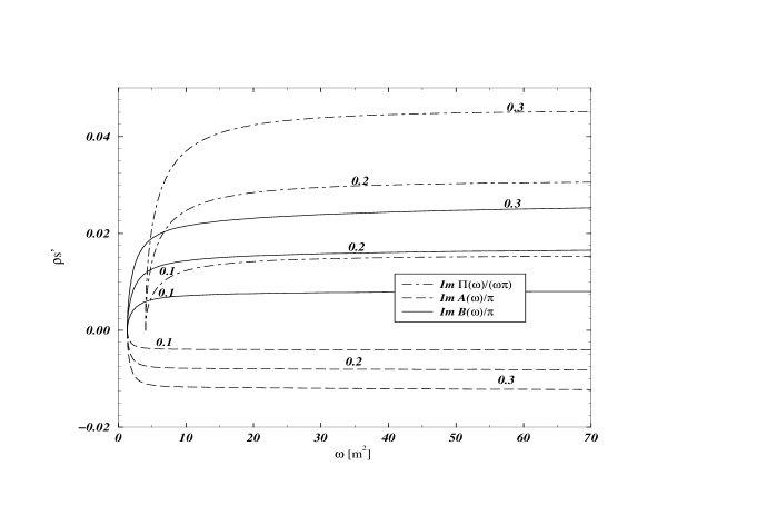
Figure 1: The spectral functions for Yukawa model calculated for the values $0.1;0.2;0.3$ of coupling strength $\lambda=\frac{g^{2}}{4\pi}$. The lines with the threshold $(m+m_{\phi})^{2}=1.15^{2}m^{2}$ correspond with the Dirac (negative lines) and scalar (positive lines). The Lehmann weights for pseudoscalar propagator have the appropriate thresholds at $4m^{2}$ and they are always positive.

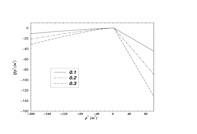
Figure 2: The self-energy of pseudoscalar meson $Q(p^{2})=m^{2}_{\phi}(\mu)+\Pi_{R}(\mu^{2},p^{2})$ for various coupling strengths $\lambda$ of Yukawa interaction. The only real part is displayed above the threshold $4m^{2}$.

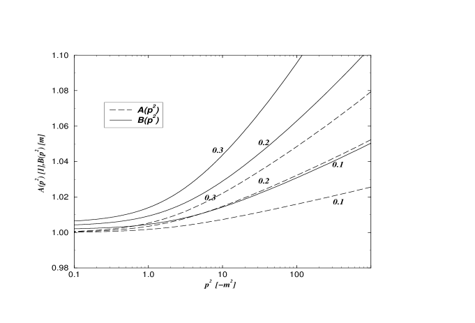
Figure 3: Yukawa fermion functions $A(p^{2}),B(p^{2})$ at space-like regime of momentum.

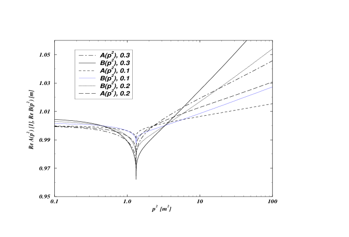
Figure 4: Yukawa fermion functions $A(p^{2}),B(p^{2})$ at time-like regime of momentum.

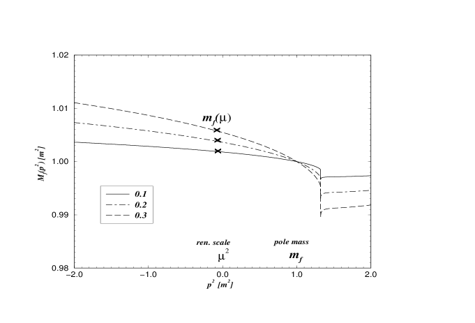
Figure 5: The renormalization scale invariant dynamical mass of Yukawa fermion. The renormalized mass $m(0)$ is fixed at $\mu=0$ such that the pole mass is $m_{f}=1$ for all the couplings $\lambda=0.1;0.2;0.3$

Fig.1 shows the absorptive parts of self-energies, i.e., the functions $\rho_{v},\rho_{s}$ for fermion and $\rho_{\phi}$ for pseudoscalar. They are plotted for the following values: $\lambda=0.1,0.2,0.3$ of the coupling strength defined as $\lambda=\frac{g^{2}}{4\pi}$. For a large momenta the spectral function $\rho_{\phi}(x)$ grows linearly with the square of momenta which is a consequence of quadratic divergence in $\Pi_{0}$. Due to this, what we actually plot is the rescaled function $\rho_{\phi}(x)/x$. All the functions start to be non zero from their perturbative thresholds- $\Im A(s),\Im B(s)$ from $s=(m_{\phi}+m)^{2}$ and $\Im\Pi(s)$ from $s=4m^{2}$. Because the negative parity of the field $\Phi$ the functions $\rho_{s},\rho_{\phi}$ (and $\sigma_{s},\sigma_{\phi}$) are positive while $\rho_{v}$ ($\sigma_{v}$) is negative. The quadratic divergence of the unrenormalized self-energy $\Pi$ leads to the quadratic dependence (+corrections) of the renormalized $\Pi$. (in fact the recent models (see for instance [49],[50]) of particle interactions attempted to avoid of quadratic divergences that necessarily follows from Yukawa sector of Standard model) The quantity $Q^{1/2}$ of dimension [mass$]^{1}$ defined with the help of eq. $Q(p^{2})=m_{\phi}^{2}(\mu)+\Pi(\mu;p^{2})$ can not be called the dynamical boson mass, since $Q$ becomes negative above the certain value of Euclidean momenta. The same happens at the time-like axis for $\Re Q(p^{2})$ (while $\Im Q(p^{2})=\pi\rho_{\phi}$ is positive as it is clear from Fig.1). The appropriate behavior of the function $Q$ is displayed in Fig.2. The momentum dependence of the fermion functions $A,B$ is dominated by the (perturbative) logarithm of $p^{2}$. Indeed, the Yukawa fermion propagator is almost given by its free form corrected by small perturbation. Fig. 3 and Fig.4 display the momentum dependence of the function $A,B$ for space-like momenta and time-like momenta respectively. Although, the smallness of the ratio $m_{phi}/m$ is motivated by the desired enhancement of fermion self-energy and subsequent suppression of pseudoscalar one, nevertheless, we still see that the fermion-meson loop becomes irrelevant perturbative contribution for all studied couplings. We display the dynamical mass $M=B/A$ in the infrared domain in the Fig.5. since this is the mainly interesting regime of momenta. The appearance of the critical coupling $\lambda_{c}$ is the consequence of the quadratic momentum dependence of pseudoscalar self-energy. Its value slightly depends on the numerical cut-off $\Lambda$ used in our unitary equation, noting that within our numeric ($\Lambda^{2}=10^{7}m^{2}$) the solution of unitary equations fails at $\lambda_{c}\simeq 0.3$.

4.2 QED fermion propagator

In contrast to the model discussed previously, the strong coupling QED is less driven by the perturbation theory (Recall here the famous paper [51] dealing with scalar electrodynamics).Before presentation of our numerical solution, let us recollect the main results:

1. Comparing the electron propagator obtained from the solution of the Unitary Equations (UEs) (3) with the propagator calculated in the Euclidean formalism we find that they never exactly agree. The exception is the case of very small coupling $\alpha\simeq 10^{-2}$, where both approaches seem to be equivalent (up to the numerical errors). Stressed here, that in this case, they are almost indistinguishable form the perturbation theory result.

2. Previous statement is valid also in the case when the small photon mass $\lambda$ is introduced. The obtained results are then slightly changed quantitatively and the disagreement discussed in 1. is somehow small (the Euclidean$\times$Minkowski results numerically agree, only when $\lambda\simeq m$, which is the case, we are not interested in). It leads us to the conclusion, that this discrepancy do not fully follows from the masslessness of the photon and from the appropriate subsequent coincidence of the electron propagator singularity with the branch point. Note, that the last property is not simply fulfilled for nonzero $\lambda$.

3. The Minkowski (spectral) solution exists only for subcritical regime of $\alpha_{QED}$, whilst, as it is well known the Euclidean solution can be easily find for both the sub- and super-critical couplings. To be more precise, we have not found any solution of UEs when the coupling was larger then $\alpha_{c.s.}=0.95$ (c.s.=critical spectral). Further, making an estimate of the momentum DSE solution (not assuming spectral decomposition) we have found strong evidence for confinement for the coupling larger then $\alpha=0.91\pm 0.1$. (Remind,that the critical coupling in QED is defined such that $B(p^{2})=0$ for $m_{0}=0$, (chiral symmetric phase) for $\alpha<\alpha_{c}$ and the solution for $B(p^{2})$ is non-zero and finite for $\alpha>\alpha_{c};m_{0}=0$ when momentum cut-off $\Lambda$ is implemented (without finite $\Lambda$ the function $B$ tends to diverge). Its value is known from the quenched, rainbow study, where $\alpha_{c}=\frac{\pi}{3}$ , more sophisticated studies do not deviate significantly from this value ).

The UEs (3) complemented by the equations for the absorptive part $\rho_{s}$ and for the residuum have been solved by the method of iterations. In order to have an infrared behavior under the control and in order to see the effect of the vector boson mass we also implement the small mass parameter $\lambda$ into the photon propagator:

$$G_{o}^{\mu\nu}(k)=\frac{-g^{\mu\nu}+k^{\mu}k^{\nu}/k^{2}}{k^{2}-\lambda^{2}+i\varepsilon}$$ (52)

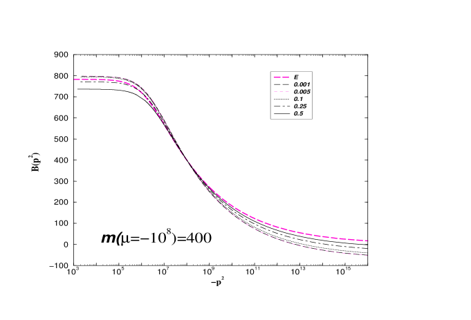
Figure 6: The dynamical mass of the electron in massive photon QED as they have been obtained by solving modified unitary equtaions. The various lines are labeled by the mass of the photon $\lambda$ which is written in the units of an on-shell electron mass. All solutions have the coupling value $\alpha=0.6$, renormalization point $\mu^{2}=-10^{8}$, and renormalized mass is $m(\mu)=400$. The results for two smallest $\lambda$ are not distinguishable. Thin long dashed line labeled by the letter E represents the solution obtained in Euclidean formalism. In this case, photon was exactly massless.

. Restricting to the small photon mass case, the Dirac part coefficient function $A$ is approximated as $A(p^{2})=1$, i.e. as it would be in the massless case. The expression for function $\rho_{s}$ is then slightly change (see Appendix A), noting here that the limit $\lambda\rightarrow 0$ is smoothly achieved as it follows from the appropriate relations (B) presented in the Appendix A. The solutions with several different photon masses have been obtained. Then, the dynamical mass $M=B$ at space-like momenta is calculated from the absorptive functions $\rho_{s},\sigma_{s},\sigma_{v}$, which are primary solutions here. We can see from the Fig.6. that the effect of the small photon mass is almost irrelevant even if the coupling is relatively large ($\alpha=0.6$). The space-like renormalization scale is chosen to be large $\mu^{2}=-10^{8}$ when compared with renormalized mass $m^{2}(\mu)=400^{2}$, which choice corresponds with the Euclidean solution already presented in the work [24]. The appropriate Euclidean solution of Eq. (3) is added for the comparison. The same (in)dependence on the parameter $\lambda$ is observed for any choice of $\mu,m(\mu)$. In order to achieve good numerical stability of UEs some very small photon mass is always used in. The presented results in this work are calculated with $\lambda=10^{-3}m$.

Solutions were obtained for the Fukuda-Kugo equation (FKE) (50) for the couplings from $0.01$ to $2.0$. The expected damping [42, 22] of dynamical mass to its negative values was observed for supercritical couplings $\alpha>\pi/3$. Using the same renormalization choice $M(0)=1$ the UEs were solved. The resulting solution for $M$ is plotted for the following couplings: $0.2,0.4,0.6$ and compared with the FKE solution. All these solutions are plotted against the space-like momentum in Fig.7. From this we can see the relatively large discrepancy between the results of FKE and UEs. Making great numerical effort we have found the main cause numerically. Let us assume that the residuum and the principal value integral integrations that appear in UE are somehow over-estimated due to the infrared enhancement of the Lehmann weights. Let us introduce small coupling constant dependent infrared cutoff $c*m^{2}$ to the UEs:

$$\sigma_{v}(\omega) = \frac{f_{1}+m(\mu)f_{2}}{\omega-m^{2}(\mu)}\quad;\quad\sigma_{s}(\omega)=\frac{m(\mu)f_{1}+\omega f_{2}}{\omega-m^{2}(\mu)}$$

$$f_{1} \equiv r\frac{m\rho_{s}(\omega)}{\omega-m^{2}}+[\sigma_{s}*\rho_{s}]\Theta(\omega-m^{2}(1+c))$$

$$f_{2} \equiv r\frac{\rho_{s}(\omega)}{\omega-m^{2}}+[\sigma_{v}*\rho_{s}]\Theta(\omega-m^{2}(1+c))$$

$$r = \left(1+m\frac{m-m(\mu)}{m(\mu)m-\mu^{2}}\right)\left(1+\int d\omega\frac{\mu^{2}\sigma_{v}(\omega)-m(\mu)\sigma_{s}(\omega)}{\omega-\mu^{2}}\right)\Theta(\omega-m^{2}(1+c))$$

$$c = \frac{\alpha}{2\pi}\,.$$ (53)

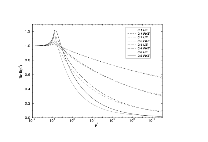
Figure 8: The electron dynamical mass $M(p^{2})=B(p^{2})$ for time-like regime of momentum and renormalization choice $m(0)=1$. The thick lines represent Euclidean solutions obtained by principal value integration of the Fukuda-Kugo equation. The thin lines correspond with the solutions of modified unitary equations (labeled by UE).

Note that taking $c=0$ then the modified unitary equations (MUEs) (4.2) clearly reproduce the originally UEs. Looking at the solutions of MUEs we see that their solutions are in the reasonable agreement with the solutions of FKE. Fig.8 displays the mass behavior at the time-like regime obtained for the same choice of renormalization mass as previous. The maximum corresponds correspond with the mass-shell point . Note that their existence is in contradiction with the assumption of confinement [42]. Although, we are pretty sure that the solution must look like as in this figure, in order to assure, we solve the time-like continued equation of Fukuda-Kugo. We were not able to find the exact and fully complex solution numerically, however, we made a sophisticated estimate of a real part of $B(p^{2})$ by the principal value integration. It is achieved by the standard numerical introduction of a finite epsilon, here it is chosen to be a fraction of pole mass and presented solutions are obtained with the choice $\epsilon=0.03m^{4}$, i.e., the singular integrand is approximated as

$$P.\frac{1}{z-B^{2}(z)}\rightarrow\frac{z-B^{2}(z)}{(z-B^{2}(z))^{2}+\epsilon}$$ (54)

where $z$ is a time-like momentum $z=p^{2}$.

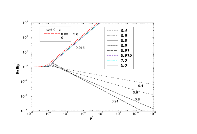
Figure 9: The same as in the previous figure, but for stronger couplings. The results are obtained from solution of Fukuda-Kugo equation only. Signal for confinement is apparent for the coupling $\alpha>0.915$. The lines represent a good estimate of true FKE solution for subcritical couplings but they must be rather exact for the supercritical couplings solutions (for the meaning of $\epsilon$ see (54)).

The soft coupling results are added to the Fig.8 and fully agree with our expectation: the branch point always exists because the mass function $B^{2}(x)$ always cuts the graph of the function $y(x)=x$. This statement is valid for QED with subcritical couplings $\alpha<0.915$. At most, we expect about ten percentage deviation from the exact value of $\alpha_{crit}$ which should be a consequence of the numerical method weakness. Furthermore, we can see from the Fig.8 that FKE solution for $\Re B$ reasonably agree with the solutions of MUEs, especially when the coupling is small enough. But we have rather different situation in strong coupling QED. The maximum of the mass function disappear and the mass function never cuts the graph $\sqrt{x}$. The supercritical coupling quenched QED is a confining theory, the electron propagator has not a branch point and is free of any singularities. In this case, $\epsilon$ introduced above can be safely limited to the zero value and we actually omitted it when FKE was solved for $\alpha>\alpha_{crit}$. The results are plotted in Fig.9 where we also add some subcritical solutions for better comparison. The subcritical solutions have been obtained with the help of time-like continued FKE and there is no spectral solutions presented in this figure (the value of infrared cut-off $c$ makes the MUEs untrusted).

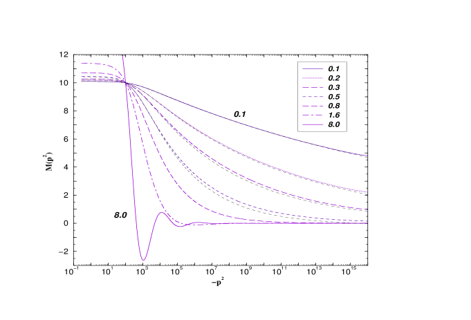
Figure 10: Space-like solutions for electron propagator. All solutions have the renormalization point $\mu^{2}=-100$, and renormalized mass $m(\mu)=10$ and couplings is varied from $0.1$ to $8.0$. Note that there are several zero-crossing when the coupling is large enough. The solutions of modified unitary equations (dashed thin lines which are closed to their Euclidean counter-partners) are added for the lowest couplings $\alpha=0.1,0.2,0.3,0.5$.

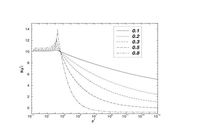
Figure 11: Time-like solution for electron propagator as they have been obtained from modified unitary equations. The renormalization choice is the same as in the previous figure, i.e. $m(-100)=10$.

The program using the Euclidean equation (3) was run with several coupling $\alpha$ from $0.2$ to $8.0$ (!), and with the renormalization choice $m(-100)=10$. Whenever $\alpha$ coincides with the one published in [22], then the results here and the ones obtained in [22] should be numerically identical. Again, we see for supercritical couplings, there is a small region where the dynamical mass is negative. When the coupling constant is extremely large (say $\alpha=8$) the negative damping becomes a relatively fast oscillation around the zero mass axis. This feature should be in agreement with [22] but in a subtle disagreement with the paper [42], where the oscillation appears to be purely positive. The solution of $B$ in space-like regime is presented in Fig.10. The solutions of MUEs and of the Euclidean momentum DSE are compared only in the space-like regime. The MUEs solutions are presented in in Fig. 11 for time-like momenta.

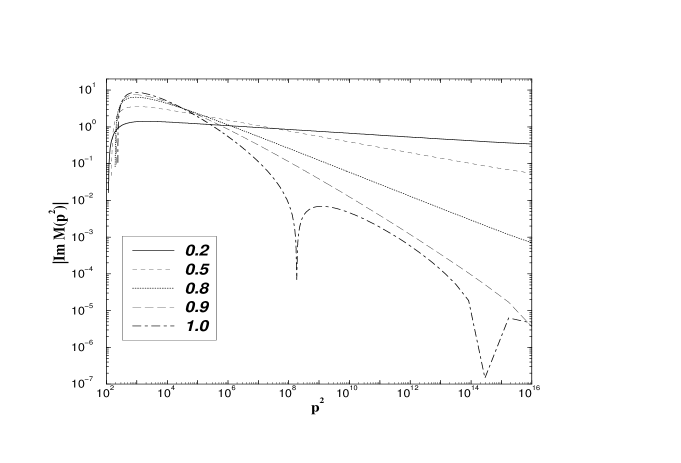
Figure 12: The absolute values of absorptive part of electron self-energy. In order to obtain the result for $\alpha=1$, we used the infrared cut-off value $0.2m$ in the modified unitary equations treatment ($m$ is a pole mass, here always $m\simeq m(-100)=10$, for instance $m=14$ for $\alpha=0.8$.

An unexpected feature of the spectral equations is that for any set $\{\alpha>0.9,\mu^{2},m(\mu)\}$ the absorptive self-energy becomes oscillating around the zero axis. This behavior was verified to be insensitive to number of grid points, but was not stable against the infrared cut-off introduced above. In fact, the positions of minima’s and maxima’s are slowly walking when the cut-off $c$ is varied by hand. The significance of this for spectral representation and its connection to QED is not completely understood. One possibility is that it may be signal the failure of Lehmann representation. The examples of this feature is shown in Fig.12. It should be emphasized here, that all the results for $M(p^{2})$ obtained by solving of MUEs and presented in this work have been calculated from non-oscillating, smoothed (soft coupling constant) $\rho_{s}$’s.

5 Conclusions and outlook

In this article we convert the Dyson-Schwinger equations for propagators to the real equations for their Lehmann weights. The possibility to do this, is based on the assumption of the existence of Green’s function integral representation which should be valid in nonperturbative regime too. They renormalized equations have been solved without some unwanted linearization or angle approximation. This is the novelty and significant advantage in comparison with the usual manner commonly used in the literature. The developed approach has been tested on two models. The QED electron propagator has been compared with the results obtained in conventional Euclidean formalism. We found certain discrepancy between these approaches which appears to be rather large when the coupling approaches its critical value. Furthermore, the solution obtained within the help of Lehmann representation is fully absent for supercritical couplings regime of QED. In this case the physical pole propagator singularity disappear and we argue that ladder QED does not describe free electrons(positrons) at all.

Acknowledgments

Author is very grateful to I.Kavková , R.Dermíšek and A.Cieplý for the careful reading of the manuscript. I also thank to prof. R.Delbourgo who point my attention on some existing literature. This research was supported by GA ČR under Contract n.202/00/1669.

Appendix A Evaluation of the off-shell dispersion relations

In this Appendix we derive the appropriate DR’s for the proper Green’s functions of YT. As a first step we analyze the fermion self-energy.

A.1 Yukawa fermion self-energy

As follows from (17) the general expression which has to be considered has the following structure:

$$\Sigma_{0}(\not\!p) = -ig^{2}\int\frac{d^{4}l}{(2\pi)^{4}}\frac{\gamma^{5}(C_{a}\not\!l+C_{b})\gamma^{5}}{(l^{2}-\alpha+i\epsilon)((l-p)^{2}-\beta+i\epsilon)}$$ (55)

$$= -ig^{2}\int\limits_{0}^{1}dx\int\frac{d^{4}l}{(2\pi)^{4}}\frac{-C_{a}\not\!p(1-x)+C_{b}}{[l^{2}+p^{2}x(1-x)-\alpha x-\beta(1-x)+i\epsilon]^{2}}\quad,$$

where the whole prefactors are absorbed into the formal symbols $C_{a,b}$ . Written in the terms of continuous functions $\sigma_{v,s}$ and Lehmann weight $\sigma$ for pseudoscalar, the symbol $C_{a}$ and $C_{b}$ are identified as

$$C_{a} = \int d\alpha\left\{\delta(\alpha-m^{2})+\sigma_{v}(\alpha)\right\}\int d\beta\left\{\delta(\beta-m_{\phi}^{2})+\sigma(\beta)\right\}$$

$$C_{b} = \int d\alpha\left\{\alpha^{1/2}\delta(\alpha-m^{2})+\sigma_{s}(\alpha)\right\}\int d\beta\left\{\delta(\beta-m_{\phi}^{2})+\sigma(\beta)\right\}$$ (56)

Noting that they should be collocated in front of the fractions in (55).

Observing the Dirac structure, the unrenormalized functions $a_{0},b_{0}$ can be simply identified. After making subtractions (2.2) we can arrive at their renormalized forms

$$a(\mu;p^{2}) = ig^{2}C_{a}\int\limits_{0}^{1}dxdy\int\frac{d^{4}l}{(2\pi)^{4}}\frac{(1-x)^{2}x2(p^{2}-\mu^{2})}{\left[l^{2}+(p^{2}-\mu^{2})x(1-x)y+\mu^{2}x(1-x)-O+i\epsilon\right]^{3}}$$

$$b(\mu;p^{2}) = -ig^{2}C_{b}\int\limits_{0}^{1}dxdy\int\frac{d^{4}l}{(2\pi)^{4}}\frac{2(1-x)x(p^{2}-\mu^{2})}{\left[l^{2}+(p^{2}-\mu^{2})x(1-x)y+\mu^{2}x(1-x)-O+i\epsilon\right]^{3}}$$

where $O=\alpha x-\beta(1-x)$. Integrating over the loop momentum and making substitution $y\rightarrow\omega$

$$\omega=\mu^{2}-\frac{\mu^{2}}{y}+\frac{O}{x(1-x)y},$$ (58)

we obtain the DR’s

$$a(\mu;p^{2}) = -C_{a}\left(\frac{g}{4\pi}\right)^{2}\int\limits_{0}^{1}dx\int\limits_{\frac{O}{x(1-x)}}^{\infty}d\omega\frac{1-x}{\omega-\mu^{2}}\frac{p^{2}-\mu^{2}}{(p^{2}-\omega+i\epsilon)}$$

$$b(\mu;p^{2}) = C_{b}\left(\frac{g}{4\pi}\right)^{2}\int\limits_{0}^{1}dx\int\limits_{\frac{O}{x(1-x)}}^{\infty}d\omega\frac{p^{2}-\mu^{2}}{\omega-\mu^{2}}\frac{1}{(p^{2}-\omega+i\epsilon)}\quad.$$ (59)

Using the following definition of X functions

$$X(\omega;\alpha,\beta) = \int\limits_{0}^{1}dx\Theta\left(\omega-\frac{O}{x(1-x)}\right)$$

$$X_{1}(\omega;\alpha,\beta) = \int\limits_{0}^{1}dxx\Theta\left(\omega-\frac{O}{x(1-x)}\right)$$ (60)

we can rewrite DR(A.1) into the more familiar form:

$$a(\mu;p^{2}) = -C_{a}\left(\frac{g}{4\pi}\right)^{2}\int d\omega\frac{X_{1}(\omega;\beta,\alpha)(p^{2}-\mu^{2})}{(\omega-\mu^{2})(p^{2}-\omega+i\epsilon)}$$

$$b(\mu;p^{2}) = C_{b}\left(\frac{g}{4\pi}\right)^{2}\int d\omega\frac{X(\omega;\alpha,\beta)(p^{2}-\mu^{2})}{(\omega-\mu^{2})(p^{2}-\omega+i\epsilon)}\quad,$$ (61)

where we made use of the relation

$$X(\omega;\alpha,\beta)-X_{1}(\omega;\alpha,\beta)=X_{1}(\omega;\beta,\alpha)\quad.$$ (62)

Explicit integrations in (A.1) give the following formulas for $X$ functions

$$X(\omega;\alpha,\beta) = \frac{\lambda^{1/2}(\alpha,\omega,\beta)}{\omega}\Theta\left(\omega-(\alpha^{\frac{1}{2}}+\beta^{\frac{1}{2}})^{2}\right)$$

$$X_{1}(\omega;\alpha,\beta) = \frac{\lambda^{1/2}(\alpha,\omega,\beta)}{2\omega}\left[1+\frac{\beta-\alpha}{\omega}\right]\Theta\left(\omega-(\alpha^{\frac{1}{2}}+\beta^{\frac{1}{2}})^{2}\right)\,,$$ (63)

where $\lambda$ is the triangle Khallén function $\lambda=(\omega-\alpha+\beta)^{2}-4\omega\beta$.

After the explicit introduction of the prefactors $C_{a,b}$ we can write down the absorptive part of self-energy functions $a,b$:

$$\rho_{a}(\omega) = \frac{-g^{2}}{(4\pi)^{2}}\left[r_{f}r_{\phi}X_{1}(\omega;{m_{\phi}}^{2},m^{2})+mr_{\phi}\int\limits_{(m+m_{\phi})^{2}}^{\infty}d\alpha\sigma_{v}(\alpha)X_{1}(\omega;m_{\phi}^{2},\alpha)\right.$$ (64)

$$+ r_{f}\int\limits_{4m^{2}}^{\infty}d\beta\rho_{\phi}(\beta)X_{1}(\omega;\beta,m^{2})$$

$$+ \left.\int\limits_{4m^{2}}^{\infty}d\beta\int\limits_{(m+m_{\phi})^{2}}^{\infty}d\alpha\rho_{\phi}(\beta)\sigma_{v}(\alpha)X_{1}(\omega;\beta,\alpha)\right],$$

$$\rho_{b}(\omega) = \frac{g^{2}}{(4\pi)^{2}}\left[r_{\phi}r_{f}mX(\omega;m_{\phi}^{2},m^{2})+r_{\phi}\int\limits_{(m+m_{\phi})^{2}}^{\infty}d\alpha\sigma_{s}(\alpha)X(\omega;m_{\phi}^{2},\alpha)\right.$$ (65)

$$+ r_{f}\int\limits_{4m^{2}}^{\infty}d\beta\rho_{\phi}(\beta)X(\omega;\beta,m^{2})$$

$$+ \left.\int\limits_{4m^{2}}^{\infty}d\beta\int\limits_{(m+m_{\phi})^{2}}^{\infty}d\alpha\rho_{\phi}(\beta)\sigma_{s}(\alpha)X(\omega;\alpha,\beta)\right].$$

As follows from the properties of function $X$ the various terms in (64),(65) start to be nonzero from different values of $\omega$. This knowledge is particularly useful when calculated numerically. Indeed after the inspection of $X(\omega;\alpha,\beta)$ we can find the threshold at $\omega=(\sqrt{\alpha}+\sqrt{\beta})$. For instance the subtresholds values $(m_{\phi}+m)^{2};(2m_{\phi}+m)^{2};9m^{2};(m_{\phi}+3m)^{2}$ correspond to the terms in Eq. (65) at given order.

A.2 Yukawa pseudoscalar self-energy

Let us find the DR for self-energy $\Pi$. The loop integral has the form:

$$\Pi(p^{2}) = i\int\frac{d^{4}l}{(2\pi)^{4}}Tr\frac{\gamma_{5}[\not\!l\bar{\sigma}_{v}(\alpha)+\bar{\sigma}_{s}](\alpha)\gamma_{5}[(\not\!l-\not\!p)\bar{\sigma}_{v}(\beta)+\bar{\sigma}_{s}(\beta)]}{(l^{2}-\alpha+i\epsilon)((l-p)^{2}-\beta+i\epsilon)}$$ (66)

$$= 4i\int\frac{d^{4}l}{(2\pi)^{4}}\left[\frac{-\bar{\sigma}_{v}(\alpha)\bar{\sigma}_{v}(\beta)}{((l-p)^{2}-\beta+i\epsilon)}\right.$$

$$+ \left.\int\limits_{0}^{1}dx\frac{(-\alpha+p^{2}(1-x))\bar{\sigma}_{v}(\alpha)\bar{\sigma}_{v}(\beta)+\bar{\sigma}_{s}(\alpha)\bar{\sigma}_{s}(\beta)}{l^{2}+p^{2}x(1-x)-O}\right],$$

where the shift $l\rightarrow l+p(1-x)$ is made at the second integral and $O=\alpha x-\beta(1-x)$. For purpose of brevity we omit the spectral integration over the variables $\alpha$ and $\beta$.

The renormalization (2.1) proceeds by direct subtracting of the first two term in Taylor expansion of unrenormalized self-energy (66). To make this explicitly we introduce shorthand notation $U(w,l,O)=(l^{2}-w^{2}(1-x)x-O+i\epsilon)$ . After a little algebra the renormalized quantity corresponding to (66) can be evaluated as

$$\Pi(\mu;p^{2}) = 4i\int\frac{d^{4}l}{(2\pi)^{4}}\int\limits_{0}^{1}dxdy\biggl{[}(-\alpha\bar{\sigma}_{v}(\alpha)\bar{\sigma}_{v}(\beta)$$ (67)

$$+ \bar{\sigma}_{s}(\alpha)\bar{\sigma}_{s}(\beta))\left(\frac{1}{U^{2}(p,l,O)}-\frac{1}{U^{2}(\mu,l,O)}+\frac{2x(1-x)(p^{2}-\mu^{2})}{U^{3}(\mu,l,O)}\right)$$

$$+ \bar{\sigma}_{v}(\alpha)\bar{\sigma}_{v}(\beta)\left(\frac{p^{2}(1-x)}{U^{2}(p,l,O)}-\frac{\mu^{2}(1-x)}{U^{2}(\mu,l,O)}+\frac{2x(1-x)^{2}\mu^{2}(p^{2}-\mu^{2})}{U^{3}(\mu,l,O)}\right)\biggr{]}.$$

Matching terms in the first line of (67) together we can rewrite them into the familiar DR

$$\frac{4g^{2}}{(4\pi)^{2}}\int d\omega\frac{X(\omega;\alpha,\beta)(-\alpha\bar{\sigma}_{v}(\alpha)\bar{\sigma}_{v}(\beta)+\bar{\sigma}_{s}(\alpha)\bar{\sigma}_{s}(\beta))(p^{2}-\mu^{2})^{2}}{(\omega-\mu^{2})^{2}(p^{2}-\omega+i\epsilon)}\quad,$$ (68)

where function $X$ was already introduced in (A.1)

The terms in the second brackets of the second line of (67) can be matched together in the following fashion:

$$\int\limits_{0}^{1}dy\left[-\frac{2(p^{2}-\mu^{2})^{2}x(1-x)^{2}}{(U(p,l,O)y+U(\mu,l,O)(1-y))^{3}}\right.+$$

$$\left.\left(2x(1-x)^{2}\mu^{2}(p^{2}-\mu^{2})\right)\left(\frac{1}{U^{3}(\mu,l,O)}-\frac{1}{(U(p,l,O)y+U(\mu,l,O)(1-y))^{3}}\right)\right]=$$

$$\int\limits_{0}^{1}dy\left[-\frac{(p^{2}-\mu^{2})^{2}(1-x)}{y\left(p^{2}-\mu^{2}+\frac{\mu^{2}}{y}-\frac{O}{x(1-x)y}\right)}\right.$$

$$+\left.\frac{(p^{2}-\mu^{2})^{2}(1-x)\mu^{2}}{\left(\mu^{2}-\frac{O}{x(1-x)y}\right)\left(p^{2}-\mu^{2}+\frac{\mu^{2}}{y}-\frac{O}{x(1-x)y}\right)}\right].$$ (69)

Adding omitted prefactors, integrating over loop momentum and making the substitution (58) in (A.2) gives rise to the DR:

$$\frac{4g_{a}^{2}}{(4\pi)^{2}}\int d\omega\frac{(X(\omega;\alpha,\beta)-X_{1}(\omega;\alpha,\beta))\omega(p^{2}-\mu^{2})^{2}}{(\omega-\mu^{2})^{2}(p^{2}-\omega+i\epsilon)}.$$ (70)

Putting all together and using the relation between $X$ and $X_{1}$ we can finally write down the DR for self-energy $\Pi$:

$$\Pi(\mu;p^{2}) = \int d\omega\frac{\rho_{\phi}(\omega)(p^{2}-\mu^{2})^{2}}{(\omega^{2}-\mu^{2})^{2}(p^{2}-\omega+i\epsilon)}$$

$$\rho_{\phi}(\omega) = \frac{4g_{a}^{2}}{(4\pi)^{2}}\int d\alpha\int d\beta\left[\left(-\alpha\bar{\sigma}_{v}(\alpha)\bar{\sigma}_{v}(\beta)+\bar{\sigma}_{s}(\alpha)\bar{\sigma}_{s}(\beta)\right)X(\omega;\alpha,\beta)\right.$$ (71)

$$+ \left.\omega X_{1}(\omega;\beta,\alpha)\bar{\sigma}_{v}(\alpha)\bar{\sigma}_{v}(\beta)\right].$$

For the purpose of numerical solution it is necessary to extract the singular parts of $\bar{SG}^{\prime}s$ explicitly. After some trivial manipulation the appropriate formula for $\rho_{\phi}$ reads

$$\rho_{\phi}(\omega)=\left(\frac{g}{2\pi}\right)^{2}\left[r_{f}^{2}\frac{\omega}{2}\sqrt{1-\frac{4m^{2}}{\omega}}\Theta(\omega-4m^{2})\right.$$ (72)

$$+ 2r_{f}m\int\limits_{(m+m_{\phi})^{2}}^{\infty}d\beta\left(\frac{1}{2}(\omega-m^{2}-\beta)\sigma_{v}(\beta)+m\sigma_{s}(\beta)\right)X(\omega;m^{2},\beta)$$

$$+ \int\limits_{(m+m_{\phi})^{2}}^{\infty}d\alpha\int\limits_{(m+m_{\phi})^{2}}^{\infty}d\beta\left(\frac{1}{2}(\omega-\alpha-\beta)\sigma_{v}(\alpha)\sigma_{v}(\beta)\right.$$

$$+ \left.\left.\sigma_{s}(\alpha)\sigma_{s}(\beta)\right)X(\omega;\alpha,\beta)\right],$$

noting that the first line of (72) corresponds with the one loop perturbative contribution.

Appendix B Quenched, rainbow, Landau gauge QED

It is shown, that with a massless photon the fermion self-energy function $b$ satisfies DR (2.2) while the function $a$ is exactly zero. In the end of this section we review the results for the case of massive photon. These are used in the numerical study described in the main text.

First we will deal with massless photon case ($\lambda=0$), where our approximate electron self-energy

$$\Sigma_{0}(\not\!p)=ie^{2}\int\frac{d^{4}k}{(2\pi)^{4}}G^{\mu\nu}_{0}(k)\gamma^{\mu}\int d{\alpha}\frac{\bar{\sigma}_{v}(\alpha)(\not\!p-\not\!k)+\bar{\sigma}_{s}(\alpha)}{(p-k)^{2}-\alpha+i\epsilon}\gamma^{\nu}\,,$$ (73)

requires one subtraction due to the presence of logarithmic ultraviolet divergence. As it is sometimes usual, we fist regularize (73), then the subtraction will follow. For this purpose we use the old-fashion Pauli-Villars regularization technique which leads to the following regularized result:

$$\Sigma_{\Lambda}(\not\!p) = -\frac{e^{2}}{(4\pi)^{2}}\int d{\alpha}\int\limits_{0}^{1}dx\left[(\bar{\sigma}_{v}(\alpha)\not\!p(4x-2)+3\bar{\sigma}_{s}(\alpha))\right.\,,$$ (74)

$$\times \ln{\left(\frac{-p^{2}x(1-x)+\alpha x+\Lambda^{2}(1-x)}{-p^{2}x(1-x)+\alpha x}+i\epsilon\right)}$$

$$+ \left.\frac{2\bar{\sigma}_{v}(\alpha)\not\!pp^{2}x^{2}(1-x)}{p^{2}x(1-x)+\alpha x}\right]\,,$$

where $\Lambda$ represents Pauli-Villars regulator. Making the aforementioned subtraction gives the renormalized functions $a,b$

$$a(\mu;p^{2}) = -\int d{\alpha}\frac{\bar{\sigma}_{v}(\alpha)e^{2}}{(4\pi)^{2}}\left[\int\limits_{0}^{1}dx(4x-2)\ln{\left(\frac{-\mu^{2}(1-x)+\alpha}{-p^{2}(1-x)+\alpha}+i\epsilon\right)}\right.$$

$$+ \left.\frac{2p^{2}}{-p^{2}(1-x)+\alpha}-\frac{2\mu^{2}}{-\mu^{2}(1-x)+\alpha}\right]$$

$$b(\mu;p^{2}) = -\int d\alpha\frac{3\bar{\sigma}_{s}(\alpha)e^{2}}{(4\pi)^{2}}\int\limits_{0}^{1}dx\ln{\left(\frac{-\mu^{2}(1-x)+\alpha}{-p^{2}(1-x)+\alpha}+i\epsilon\right)}.$$ (75)

where $\mu^{2}$ is space-like renormalization scale. The per-partes integration of logarithm terms gives

$$a(\mu;p^{2}) = 0$$

$$b(\mu;p^{2}) = \int d\alpha\frac{3\bar{\sigma}_{s}(\alpha)e^{2}}{(4\pi)^{2}}\int\limits_{0}^{1}dx\frac{x}{(1-x)}\frac{p^{2}}{(p^{2}-\frac{\alpha}{1-x}+i\epsilon)}-(p^{2}\rightarrow\mu^{2})$$ (76)

$$= -\left(\frac{3e}{4\pi}\right)^{2}\int d\alpha\int\limits_{\alpha}^{\infty}d\omega\frac{3\bar{\sigma}_{s}(\alpha)(1-\frac{\alpha}{\omega})(p^{2}-\mu^{2})}{(\omega-\mu^{2})(p^{2}-\omega+i\epsilon)}\,,$$

Thus absorptive part of self-energy $\pi\rho$ is given by :

$$\rho_{s}(\omega)=-3\left(\frac{e}{4\pi}\right)^{2}\left[r\,m\left(1-\frac{m^{2}}{\omega}\right)+\int_{m^{2}}^{\omega}d\alpha\sigma_{s}(\alpha)\left(1-\frac{\alpha}{\omega}\right)\right].$$ (77)

Note here, that the Pauli-Villars regularization technique was chosen for convenience only. It is not so difficult to use, for instance, the dimensional regularization technique. Of course, making direct algebraic subtraction of unregularized $a,b$ is also possible. All these purely technically different approaches leads to the same results, that is the subject what we exactly understand under the statement ”regularization independence”.

When the photon propagator $G_{o}$ is changed by the introduction of small mass parameter $\lambda$

$$G_{o}^{\mu\nu}(k)=\frac{-g^{\mu\nu}+k^{\mu}k^{\nu}/k^{2}}{k^{2}-\lambda^{2}+i\varepsilon}$$ (78)

then the previous results are slightly modified. Repeating the steps as above it leads to the same form of dispersion relation (2.2) but with different $\rho_{s}$,$\rho_{v}$ , both of them are nonzero now. We get for them

$$\rho_{s}(\omega) = -3\left(\frac{e}{4\pi}\right)^{2}\left\{mX(\omega,m^{2},\lambda^{2})+\int d\alpha\sigma_{s}(\alpha)X(\omega,\alpha,\lambda^{2})\right\}$$

$$\rho_{v}(\omega) = \left(\frac{e}{4\pi}\right)^{2}\Biggl{\{}X(\omega,m^{2},\lambda^{2})-2X_{1}(\omega,m^{2},\lambda^{2})$$ (79)

$$+ (\omega-m^{2})\frac{X_{1}(\omega,m^{2},\lambda^{2})-2X_{1}(\omega,m^{2},0)}{\lambda^{2}}+\int d\alpha\sigma_{s}(\alpha)\Bigl{[}X(\omega,\alpha,\lambda^{2})$$

$$- 2X_{1}(\omega,\alpha,\lambda^{2})+(\omega-\alpha)\frac{X_{1}(\omega,\alpha,\lambda^{2})-2X_{1}(\omega,\alpha,0)}{\lambda^{2}}\Bigr{]}\Biggr{\}}$$

Stressed here, that the limit $\lambda\rightarrow 0$ can be safely performed an leads to the result (77) and $\rho_{v}=0$.

Appendix C Numerical details

The unitary equations have been solved by the method of numerical iteration. To achieve a reasonable accuracy we should carefully perform the principal value integrations labeled by $[\sigma,\rho],([\sigma,\rho])$ in the equation for fermion (pseudoscalar) weights. For instance the numerical P. integration

$$[\sigma*\rho]=P.\int\limits_{thresh.}^{\infty}dx\frac{\sigma(s)\rho(x)\frac{s-\mu^{2}}{x-\mu^{2}}+\sigma(x)\rho(s)}{s-x}.$$ (80)

is proceed by the following way which is based on the exact relation $0=\int\limits_{0}^{\infty}dx\frac{1}{x^{2}-a^{2}}$. Hence we can write for P. integral in (80):

$$P.\int\limits_{c}^{\infty}dx\frac{f(x)}{a-x}=P.\int\limits_{c}^{\infty}dx\frac{f(x)(a+x)-f(a)2a}{a^{2}-x^{2}}+f(a)\ln(\frac{a-c}{a+c})$$ (81)

where

$$f(x)=\sigma(a)\rho(x)\frac{a-\mu^{2}}{x-\mu^{2}}+\sigma(x)\rho(a).$$

The right hand side of the identity (81) is particularly useful when evaluated numerically i.e., when $\int\rightarrow\Sigma$.

Using some contemporary PC machine the criterion $\sigma^{2}_{n,n-1}\simeq 10^{-18}$ can be achieved, noting that the typical CPU time is about $10^{2}s$ for a grid number of several hundred mesh points. Here, $\sigma^{2}_{n,n-1}$ represents the error between the solution of $n$ times and $n-1$ times iterated unitary equation i.e.,

$$\sigma^{2}_{n,n-1}=\frac{\int(\rho_{n}^{2}-\rho_{n-1}^{2})}{\int(\rho_{n}^{2}+\rho_{n-1}^{2})}.$$ (82)

Figure 7: The electron dynamical mass $M(p^{2})$ for space-like regime of momentum. Six dotted lines represent the Euclidean solutions of momentum DSE. They are labeled by the value of coupling constant at given order (from up to down). The solutions of unitary equations (dot dashed lines) and the ones of modified unitary equations (solid thin lines) are added for the coupling $\alpha=0.2;0.4;0.6$.

References

- [1] F.J.Dyson, The S Matrix In Quantum Electrodynamics, Phys. Rev. 75, 1736 (1949).
- [2] J.Schwinger, On the Green’s Functions of Quantized Fields. 1., Proc.Natl.Acad.Sci. U.S.A. 37, 452 (1951).
- [3] L.von Smekal, R. Alkofer, The Infrared Behavior of QCD Green’s Functions - Confinement, Dynamical Symmetry Breaking, and Hadrons as Relativistic Bound States, Phys. Rept. 353, 281 (2001).
- [4] C.D. Roberts and A.G.Williams, Dyson-Schwinger Equations and the Application to Hadronic Physics, Prog. Part. Nucl. Phys. 33, 477 (1994) .
- [5] P. Maris and C.D. Roberts , Dyson-Schwinger Equations: A Tool for Hadron Physics, nucl-th/0301049.
- [6] Craig D. Roberts, Nonperturbative effects in QCD at Finite Temperature and Density, Prog. Part. Nucl. Phys. 30, 223 (1999).
- [7] A. Cohen and H. Georgi, Walking Beyond the Rainbow, Nucl. Phys. B 314, 7 (1989).
- [8] W. Barden, C.N. Leung, and S.T. Love, Aspects of Dynamical Symmetry Breaking in Gauge Field Theories, Nucl. Phys. B 323, 493 (1989).
- [9] S.F. King, Dynamical Electroweak Symmetry Breaking, Rept.Prog.Phys. 58, 263 (1995).
- [10] John M. Cornwall, Dynamical Mass Generation In Continuum QCD, Phys. Rev. D 26, 1453 (1982).
- [11] J.M. Cornwall and J. Papavassiliou, Gauge Invariant Three Gluon Vertex In QCD , Phys. Rev. D 40, 3474 (1989).
- [12] D. Binosi and J. Papavassiliou, Gauge-Independent Off-Shell Fermion Self-Energies at Two Loops: The Cases of QED and QCD , Phys. Rev. D 65, 085003 (2002).
- [13] A. Denner, G. Weiglein and S. Dittmaier, Application of the Background Field Method to the Electroweak Standard Model, Nucl.Phys. B440, 95 (1995) and references therein.
- [14] J.S. Ball and T-W. Chiu, Analytic properties of the vertex function in gauge theories 1.,Phys. Rev. D 22, 2542 (1980).
- [15] A. Salam, Renormalizable Electrodynamics Of Vector Mesons. Phys. Rev. 130, 1287 (1963).
- [16] R.Delbourgo, Gauge Technique, Nuovo Cimento 49, 484 (1979).
- [17] R.Delbourgo and R.B.Zhang,Transverse vertices in Electrodynamics and the Gauge Technique, J. Phys. A 17, 3593 (1984), and refeences therein.
- [18] Y. Hoshino,A gauge covariant approximation to QED, hep-th/0202020.
- [19] D.C. Curtis and M.R. Pennington, Truncating The Schwinger-Dyson Equations: How Multiplicative Renormalizability and the Ward identity Restrict the Three point vertex in QED,Phys. Rev. D 42, 4165 (1990).
- [20] D.C. Curtis and M.R. Pennington, Nonperturbative Study Of The Fermion Propagator In Quenched QED In Covariant Gauges using a Renormalizable Truncation of Schwinger-Dyson Equation, Phys. Rev. D 48, 4933 (1993).
- [21] D.Atkinson, J.C.R. Bloch, V.P. Gusynin, M.R. Pennington, M. Reenders Strong QED With Weak Gauge Dependence: Critical Coupling and Anomalous Dimension,Phys. Lett. B 329, 117 (1994).
- [22] F.T.Hawes, T.Sizer and A.G.Williams, Chiral Symmetry Breaking in Quenched Massive Strong-Coupling 4D QED, Phys. Rev. D 51, 3081 (1995).
- [23] F.T.Hawes, T.Sizer and A.G.Williams,On Renormalized Strong-Coupling Quenched QED in Four Dimensions, Phys. Rev. D 55, 3866 (1997).
- [24] A.W.Schreiber, T.Sizer and A.G.Williams, Dimensionally regularized study of nonperturbative quenched QED, Phys. Rev. D 58, 125014 (1998).
- [25] A.Kizilersu, T.Sizer, A.G.Williams, Regularization-independent study of renormalized non-perturbative quenched QED, Phys.Rev. D65, 085020 (2002).
- [26] S. Wu, H. X. Zhang, Y. J. Yao, Coupled Dyson-Schwinger Equations and Effects of Self-Consistency, Nucl.Phys., 694A, 489 (2001).
- [27] A. Blumhofer and J. Manus, New Insight in Dynamical Symmetry Breaking via Imaginary Part Analysis, Nucl.Phys. 515B, 522 (1998).
- [28] V.Šauli , J. Adam , hep-ph/0111433 , accepted for publication in Phys. Rev. D.
- [29] V.Šauli, J.Adam ,Solving The Schwinger-Dyson Equation For A Scalar Propagator in Minkowski space, Nucl. Phys. 689A, 467 (2001).
- [30] V.Šauli,Non-perturbative solution of metastable scalar models, hep-ph/0211221. .
- [31] A.Kizilersu, A.W.Schreiber, A.G.Williams,Regularization-independent studies of nonperturbative field theory, Phys.Lett. 499B, 261 (2001).
- [32] D. Atkinson and J.C.R. Bloch, QCD in the Infrared with Exact Angular Integrations, Mod.Phys.Lett. A 13, 1055 (1998).
- [33] S.F.Edwards, A Nonperturbation Approach to Quantum Electroynamics, Phys. Rev. 90, 284 (1953).
- [34] R.Delbourgo, A.C.Kalloinatis and G. Thoompson, Dimensional renormalization: ladders to rainbows, Phys. Rev. D 54, 5373 (1996).
- [35] H. Lehmann, On the Properties of Propagation Functions and Renormalization Constants of Quantized Fields, Nuovo cimento, 11, 342 (1954).
- [36] G.Kallen, Quantenelektrodynamik,in ”Handbuch der Physik,” Vol.5, Part I. J.Springer Verlag,Berlin ,1958; also Kgl. Danke Viedenskab. Selskab, Mat.fys. Medd. 27, No.12 (1953);
- [37] N. Nakanishi, Graph Theory and Feynman Integrals, (eds. Gordon and Breach, New York,1971).
- [38] C. Itzykson and J-B. Zuber, Quantum Field Theory, McGraw-Hill (1980).
- [39] Silvan S. Schweber, An Introduction to Relativistic Quantum Field Theory, Row, Peterson and Co*Evanston, Ill., Elmsford, N.Y. (1961).
- [40] J.M. Cornwall, Confinement and Chiral Symmetry Breakdown: Estimates of and effective quark masses. Phys.Rev. D 22, 1452 (1980).
- [41] P. Maris, Confinemet and complex singularities in QED3, Phys.Rev. D 52, 6087 (1995).
- [42] R.Fukuda and T.Kugo, Schwinger-Dyson equation for massless vector theory and the absence of a fermion pole, Nucl. Phys. B 117, 250 (1976).
- [43] Kei-Ichi Kondo, Existence of confinement phase in quantum electrodynamics, Phys.Rev. D58, 085013 (1998).
- [44] D. Atkinson and D.W.E Blatt, Determination of the Singularities of thr Electron Poropagator, Nucl. Phys. B 151, 342 (1979).
- [45] P. Maris, Analytical structure of the full fermion propagator in quenched and unquenched QED, Int.J.Mod.Phys. A 7, 5369 (1992).
- [46] W. Celmaster and D.Sivers, Studies in the Renormalization Prescription Dependence of Perturbation Calculations, Phys. Rev. D 23, 227 (1981).
- [47] V.Šauli, in preparation.
- [48] H. Georgi, E.T. Simmons and A.G. Cohen, Finding Gauges Where Z(p) Equals One, Phys.Lett. B236, 183 (1990).
- [49] N.Arkani-Hamed, A.G. Cohen, E.Katz, A.E.Nelson The Littlest Higgs, JHEP 0207, 034 (2002).
- [50] T. Han, H.E. Logan, B. McElrath, Lian-Tao Wang, Phenomenology of the Little Higgs Model,hep-ph/0301040.
- [51] S. Coleman and E. Weinberg, Radiative Corrections as the Origin of Spontaneous Symmetry Breaking, Phys. Rev. D7, 1888 (1973).
- [52] H. Bateman, A. Erdélyi, Higher Transcedental Functions III. , New York-Toronto-London. McGraw-Hill (1955).