The doubly heavy baryons

Abstract

We present the results for the masses of the doubly heavy baryons $\Xi_{QQ^{\prime}}$ and $\Omega_{Q^{\prime}Q}$ where $Q,Q^{\prime}=b,c$ obtained in the framework of the simple approximation within the nonperturbative string approach.

Doubly heavy baryons are baryons that contain two heavy quarks, either $cc$, $bc$ or $bb$. Their existence is a natural consequence of the quark model of hadrons, and it would be surprising if they did not exist. In particular, data from the BaBar and Belle collaborations at the SLAC and KEK B-factories would be good places to look for doubly charmed baryons. Recently the SELEX, the charm hadroproduction experiment at Fermilab, reported a narrow state at $3519\pm 1$ MeV decaying in $\Lambda_{c}^{+}K^{-}\pi^{+}$, consistent with the weak decay of the doubly charged baryon $\Xi_{cc}^{+}$ [1]. The candidate is $6.3\sigma$ signal. Another candidate particle is related by the replacement of a down by an up quark, so the mass difference is expected to be similar to that of the proton and neutron. SELEX, however, sees a mass difference 60 times larger [2]. Whether or not the states that SELEX reports turn out to be the first observation of doubly charmed baryons, studying their properties is important for a full understanding of the strong interaction between quarks.

The purpose of this talk is to present the results of the calculation [3] of the masses of the doubly-heavy baryons obtained in a simple approximation within the nonperturbative QCD (for a recent review see [4] and references therein). The starting point of the approach is the Feynman-Schwinger representation for the Green function of the three quarks propagating in the nonperturbatibe confining background. The role of the time parameter along the trajectory of each quark is played by the Fock-Schwinger proper time. The proper and real times for each quark related via a new quantity that eventually plays the role of the dynamical quark mass. The final result is the derivation of the Effective Hamiltonian, see Eq. (2) below. In contrast to the standard approach of the constituent quark model the dynamical masses $m_{i}$ are no longer free parameters. They are expressed in terms of the running masses $m^{(0)}_{i}$ defined at the appropriate scale of $\mu\sim 1$ GeV from the condition of the minimum of the baryon mass $M_{B}$ as function of $m_{i}$:

$$\frac{\partial M_{B}(m_{i})}{\partial m_{i}}=0.$$ (1)

Technically, this has been done using the einbein (auxiliary fields) approach, which is proven to be rather accurate in various calculations for relativistic systems.

This method was already applied to study baryon Regge trajectories [5] and very recently for computation of magnetic moments of light baryons [6]. The essential point of this talk is that it is very reasonable that the same method should also hold for hadrons containing heavy quarks. As in [6] we take as the universal parameter the QCD string tension $\sigma$. We also include the perturbative Coulomb interaction with the frozen coupling $\alpha_{s}(\text{1 GeV})=0.4$.

From experimental point of view, a detailed discussion of the excited $QQ^{\prime}q$ states is probably premature. Therefore we consider the ground state baryons without radial and orbital excitations in which case tensor and spin-orbit forces do not contribute perturbatively. Then only the spin-spin interaction survives in the perturbative approximation. The EH has the following form

$$H=\sum\limits_{i=1}^{3}\left(\frac{m_{i}^{(0)2}}{2m_{i}}+\frac{m_{i}}{2}\right)+H_{0}+V,$$ (2)

where $H_{0}$ is the non-relativistic kinetic energy operator, $m_{i}^{(0)}$ are the current quark masses and $m_{i}$ are the dynamical quark masses to be found from (1), and $V$ is the sum of the perturbative one gluon exchange potential $V_{c}$ and the string potential $V_{\text{string}}$. The string potential has been calculated in [5] as the static energy of the three heavy quarks: $V_{\text{string}}(\boldsymbol{r}_{1},\boldsymbol{r}_{2},\boldsymbol{r}_{3})=\sigma R_{\text{min}}$, where $R_{\text{min}}$ is the sum of the three distances $|\boldsymbol{r}_{i}|$ from the string junction point.

The baryon wave function depends on the three-body Jacobi coordinates

$$\boldsymbol{\rho}_{ij}=\sqrt{\frac{\mu_{ij}}{\mu}}(\boldsymbol{r}_{i}-\boldsymbol{r}_{j}),$$ (3)

$$\boldsymbol{\lambda}_{ij}=\sqrt{\frac{\mu_{ij,k}}{\mu}}\left(\frac{m_{i}\boldsymbol{r}_{i}+m_{j}\boldsymbol{r}_{j}}{m_{i}+m_{j}}-\boldsymbol{r}_{k}\right)$$ (4)

($i,j,k$ cyclic), where $\mu_{ij}$ and $\mu_{ij,k}$ are the appropriate reduced masses

$$\mu_{ij}=\frac{m_{i}m_{j}}{m_{i}+m_{j}},~{}~{}\mu_{ij,k}=\frac{(m_{i}+m_{j})m_{k}}{m_{i}+m_{j}+m_{k}},$$ (5)

and $\mu$ is an arbitrary parameter with the dimension of mass which drops off in the final expressions.

In terms of the Jacobi coordinates the kinetic energy operator $H_{0}$ is written as

$$H_{0} = -\frac{1}{2\mu}\left(\frac{\partial^{2}}{\partial\boldsymbol{\rho}^{2}}+\frac{\partial^{2}}{\partial\boldsymbol{\lambda}^{2}}\right)$$ (6)

$$=-\frac{1}{2\mu}\left(\frac{\partial^{2}}{\partial R^{2}}+\frac{5}{R}\frac{\partial}{\partial R}+\frac{K^{2}(\Omega)}{R^{2}}\right),$$

where $R$ is the six-dimensional hyper-radius

$$R^{2}=\boldsymbol{\rho}^{2}+\boldsymbol{\lambda}^{2},$$ (7)

and $K^{2}(\Omega)$ is angular momentum operator whose eigen functions (the hyperspherical harmonics) are

$$K^{2}(\Omega)Y_{[K]}=-K(K+4)Y_{[K]},$$ (8)

with $K$ being the grand orbital momentum. In terms of $Y_{[K]}$ the wave function $\psi(\boldsymbol{\rho},\boldsymbol{\lambda})$ can be written in a symbolical shorthand as

$$\psi(\boldsymbol{\rho},\boldsymbol{\lambda})=\sum\limits_{K}\psi_{K}(R)Y_{[K]}(\Omega).$$

In the hyper radial approximation which we shall use below $K=0$ and $\psi=\psi(R)$. Note that the centrifugal potential in the Schrödinger equation for the radial function $\chi(R)=R^{5/2}\psi_{K}(R)$ with a given $K$

$$\frac{(K+2)^{2}-1/4}{R^{2}}$$

is not zero even for $K=0$.

In terms of the $\boldsymbol{\rho}$ and $\boldsymbol{\lambda}$ the potential $V_{\text{string}}(\boldsymbol{r}_{1},\boldsymbol{r}_{2},\boldsymbol{r}_{3})$ has rather complicated structure. Let $\theta_{ijk}$ be the angle between the line from quark $i$ to quark $j$ and that from quark $j$ to quark $k$. If $\theta_{ijk}$ are all smaller than 120^o, then the equilibrium junction position ${\bf Y}$ is

$${\bf Y}={\bf R}_{cm}+\alpha\boldsymbol{\rho}+\beta\boldsymbol{\lambda},$$ (9)

where

$$\alpha =\frac{1}{2}\sqrt{\frac{\mu}{\mu_{ij}}}\left(\frac{m_{j}-m_{i}}{m_{i}+m_{j}}-\frac{1}{\sqrt{3}}\cdot\frac{4t+(3-t^{2})\cot\chi}{1+t^{2}}\right),$$

$$\beta =\frac{\sqrt{\mu\mu_{ij,k}}}{m_{i}+m_{j}}+\sqrt{\frac{\mu}{3\mu_{ij}}}\cdot\frac{\rho}{2\lambda\sin\chi}\cdot\frac{3-t^{2}}{1+t^{2}},$$

where

$$t=\frac{2\lambda\sin\chi+\sqrt{\dfrac{3\mu_{ij,k}}{\mu_{ij}}}\rho}{2\lambda\cos\chi+\sqrt{\dfrac{3\mu_{ij,k}}{\mu_{ij}}}\cdot\dfrac{m_{j}-m_{i}}{m_{i}+m_{j}}\rho},$$

and $\chi$ is the angle between $\boldsymbol{\rho}$ and $\boldsymbol{\lambda}$. If $\theta_{ijk}$ is equal to or greater than 120^o, the lowest energy configuration has the junction at the position of quark $j$. It can be easily seen that dependence on $m_{i}$ in equations (9) is apparent and $\boldsymbol{Y}$ does not depend on quark masses as it should be.

Table 1: The constituent quark masses $m_{i}$ and the ground state eigenvalues $E_{0}$ (in units of GeV) for the various baryon states.

baryon	$m_{1}$	$m_{2}$	$m_{3}$	$E_{0}$
(qqq)	0.372	0.372	0.372	1.426
(qqs)	0.377	0.377	0.415	1.398
(qss)	0.381	0.420	0.420	1.370
(sss)	0.424	0.424	0.424	1.343
(qqc)	0.424	0.424	1.464	1.171
(qsc)	0.427	0.465	1.467	1.146
(ssc)	0.468	0.468	1.469	1.121
(qqb)	0.446	0.446	4.819	1.085
(qsb)	0.448	0.487	4.820	1.059
(ssb)	0.490	0.490	4.821	1.033
(qcc)	0.459	1.498	1.498	0.904
(scc)	0.499	1.499	1.499	0.881
(qcb)	0.477	1.524	4.834	0.783
(scb)	0.517	1.525	4.834	0.759
(qbb)	0.495	4.854	4.854	0.593
(sbb)	0.534	4.855	4.855	0.570

In what follows the string junction point is chosen as coinciding with the center–of–mass coordinate. Accuracy of this approximation that greatly simplifies the calculations was discussed in [5]. Averaging the interaction $V=V_{c}+V_{\text{string}}$ over the six-dimensional sphere one obtains the Schrödinger equation for $\chi(R)$

$$\frac{d^{2}\chi(R)}{dR^{2}}+2\mu\left[E_{0}+\frac{a}{R}-bR-\frac{15}{8\mu R^{2}}\right]\chi(R)=0,$$ (10)

where $E_{0}$ is the ground state eigenvalue and

$$a=\frac{2\alpha_{s}}{3}\cdot\frac{16}{3\pi}\cdot\frac{1}{\sqrt{\mu}}\cdot\left(\sum\limits_{i<j}\sqrt{\mu_{ij}}\right),$$ (11)

$$b=\sigma\cdot\frac{32}{15\pi}\cdot\sqrt{\mu}\cdot\left(\sum\limits_{i<j}\frac{\sqrt{\mu_{ij,k}}}{m_{k}}\right),$$ (12)

We use $\sigma=0.15\text{~{}GeV}^{2}$, $\alpha_{s}=0.39$, $m^{(0)}_{q}=0.009$ GeV, $m^{(0)}_{s}=0.17$ GeV, $m^{(0)}_{c}=1.4$ GeV, and $m^{(0)}_{b}=4.8$ GeV, slightly different from [3]. We solve Eq. (10) by the variational method introducing a simple variational Ansätz

$$\chi(R)\sim R^{5/2}e^{-\mu p^{2}R^{2}},$$ (13)

where $p$ is the variational parameter. Then the three-quark Hamiltonian admits explicit solutions for the energy and the ground state eigenfunction: $E\approx\min\limits_{p}E(p)$, where

$$E(p) = \langle\chi|H|\chi\rangle=3p^{2}$$ (14)

$$-a\sqrt{\mu}\cdot\frac{3}{4}\sqrt{\frac{\pi}{2}}\cdot p+\frac{b}{\sqrt{\mu}}\cdot\frac{15}{16}\frac{\sqrt{\frac{\pi}{2}}}{p}.$$

We first solve Eq. (1) for the dynamical masses $m_{i}$ retaining only the string potential in the effective Hamiltonian (2). This procedure is in agreement with the strategy adopted in Ref. [6]. Then we add the perturbative Coulomb potential and solve Eq. (2) to obtain the ground state eigenvalues $E_{0}$. The results for various baryons are given in Table 1. The dynamical values of light quark mass $m_{q}\sim\sqrt{\sigma}\sim~{}400-500$ MeV ($q=u,d,s$) qualitatively agree with the results of Ref. [7] obtained from the analysis of the heavy–light ground state mesons. For the heavy quarks ($Q~{}=~{}c$ and $b$) the variation in the values of their dynamical masses $m_{Q}$ is marginal. This is illustrated by the simple analytical results for Qud baryons. These results were obtained from the approximate solution of equation

$$\frac{\partial E_{0}}{\partial p}=0$$ (15)

in the form of expansion in the small parameters

$$\xi=\frac{\sqrt{\sigma}}{m_{Q}^{(0)}}~{}~{}{\rm and}~{}~{}\alpha_{s}.$$ (16)

Omitting the intermediate steps one has

$$E_{0}=3\sqrt{\sigma}\left(\frac{6}{\pi}\right)^{1/4}\left(1+A\cdot\xi-\frac{5}{3}B\cdot\alpha_{s}+\dots\right)$$ (17)

$$m_{q}=\sqrt{\sigma}\left(\frac{6}{\pi}\right)^{1/4}\left(1-A\cdot\xi+B\cdot\alpha_{s}+\dots\right),$$ (18)

$$m_{Q}=m_{Q}^{(0)}\left(1+{\cal O}(\xi^{2},\alpha_{s}^{2},\alpha_{s}\xi)+\dots\right),$$ (19)

where for the Gaussian variational Ansätz (13)

$$A=\frac{\sqrt{2}-1}{2}\left(\frac{6}{\pi}\right)^{1/4}\approx 0.24,~{}B=\frac{4+\sqrt{2}}{18}\sqrt{\frac{6}{\pi}}\approx 0.42.$$ (20)

Note that the corrections of the first order in $\xi$ and $\alpha_{s}$ are absent in the expression (19) for $m_{Q}$. Accuracy of this approximation is illustrated in Table 1 of Ref. [8].

Table 2: Masses of doubly heavy baryons

State	this work	[10]	[11]	[12]	[13]
$\Xi\{qcc\}$	3.64	3.70	3.71	3.66	3.48
$\Omega\{scc\}$	3.82	3.80	3.76	3.74	3.58
$\Xi\{qcb\}$	6.93	6.99	6.95	7.04	6.82
$\Omega\{scb\}$	7.10	7.07	7.05	7.09	6.92
$\Xi\{qbb\}$	10.14	10.24	10.23	10.24	10.09
$\Omega\{sbb\}$	10.31	10.30	10.32	10.37	10.19

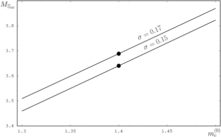
Figure 1: Mass of $\Xi_{cc}^{+}$ as a function of the running $c$–quark mass for $\sigma=0.15\text{~{}GeV}^{2}$ and $\sigma=0.17\text{~{}GeV}^{2}$. The masses are given in GeV. Bold points refer to the case $m_{c}^{(0)}=1.4\text{~{}GeV}$

To calculate hadron masses we, as in Ref. [5], first renormalize the string potential:

$$V_{\text{string}}\to V_{\text{string}}+\sum\limits_{i}C_{i},$$ (21)

where the constants $C_{i}$ take into account the residual self-energy (RSE) of quarks [9]. In what follows we adjust the RSE constants $C_{i}$ to reproduce the center-of-gravity for baryons with a given flavor. As a result we obtain $C_{q}=0.30\text{~{}GeV}$, $C_{s}=0.15\text{~{}GeV}$, $C_{c}\sim C_{b}\sim 0.$

We keep these parameters fixed to calculate the masses given in Table 2, namely the spin–averaged masses (computed without the spin–spin term) of the lowest double heavy baryons. In this Table we also compare our predictions with the results obtained using the additive non–relativistic quark model with the power-law potential [10], relativistic quasipotential quark model [11], the Feynman-Hellmann theorem [12] and with the predictions obtained in the approximation of double heavy diquark [13]. The change of $\sigma$ to $0.17\text{~{}GeV}^{2}$ increases the mass of $\Xi_{cc}^{+}$ by $\sim 30$ MeV. The perturbative spin-spin interaction introduces an additional shift of the $\Xi_{cc}^{+}$ mass $\sim-20$ MeV. Note that the mass of $\Xi_{cc}^{+}$ is rather sensitive to the value of the running $c$-quark mass $m_{c}^{0}$, see Fig.1.

In conclusion, we have employed the general formalism for the baryons, which is based on nonperturbative QCD and where the only inputs are $\sigma$, $\alpha_{s}$ and two additive constants, $C_{q}$ and $C_{s}$, the residual self–energies of the light quarks. Using this formalism we have also performed the calculations of the spin–averaged masses of baryons with two heavy quarks. One can see from Table 2 that our predictions are especially close to those obtained in Ref. [10] using a variant of the power–law potential adjusted to fit ground state baryons.

References

- [1] M.Mattson et al., Phys. Rev. Lett. 89 (2002) 112001
- [2] P.S.Cooper, these Proceedings
- [3] I.M.Narodetskii and M.A.Trusov, Phys. Atom. Nucl. 65 (2002) 917 [hep-ph/0104019]
- [4] Yu.A.Simonov, hep-ph/0205331
- [5] M.Fabre de la Ripelle and Yu.A.Simonov, Ann. Phys. (N.Y.) 212 (1991) 235
- [6] B.O.Kerbikov, Yu.A.Simonov, Phys. Rev. D62, 093016 (2000).
- [7] Yu.S.Kalashnikova and A.Nefediev, Phys. Lett. B 492 (2000) 91
- [8] I.M.Narodetskii and M.A.Trusov, in Proceedings of the 9th International Conference on the Structure of Baryons (Baryons-2002), 3-8 March, 2002, Newport News, VA, USA, [hep-ph/0304320]
- [9] Yu.A.Simonov, Phys.Lett. B515 (2001) 137
- [10] E.Bagan et al. Z.Phys. C 64 (1994) 57
- [11] D.Ebert et al., Z. Phys. C 76 (1997) 111
- [12] R.Roncaglia et al., Phys. Rev. D 52 (1995) 1248
- [13] A.K.Likhoded and A.I.Onishchenko, hep-ph/ 9912425