CERN-TH/2002-221

UMN–TH–2112/02

TPI–MINN–02/41

hep-ph/0209036

September 2002

Stable, Time-Dependent, Exact Solutions for
Brane Models with a Bulk Scalar Field

Panagiota Kanti${}^{\,(a)}$, Seokcheon Lee${}^{\,(b)}$ and Keith A. Olive${}^{\,(b,c)}$

${}^{\,(a)}$Theory Division, CERN, CH-1211 Geneva 23, Switzerland

${}^{\,(b)}$School of Physics and Astronomy,
University of Minnesota, Minneapolis, MN 55455, USA

${}^{\,(c)}$Theoretical Physics Institute,
University of Minnesota, Minneapolis, MN 55455, USA

Abstract

We derive two classes of brane-world solutions arising in the presence of a bulk scalar field. For static field configurations, we adopt a time-dependent, factorizable metric ansatz that allows for radion stabilization. The solutions are characterized by a non-trivial warping along the extra dimension, even in the case of a vanishing bulk cosmological constant, and lead to a variety of inflationary, time-dependent solutions of the 3D scale factor on the brane. We also derive the constraints necessary for the stability of these solutions under time-dependent perturbations of the radion field, and we demonstrate the existence of phenomenologically interesting, stable solutions with a positive cosmological constant on the brane.

1 Introduction

Over the last few years, there has been considerable interest in models in which our universe is a 3-brane (a hyper-surface) embedded in a higher dimensional bulk. Much of the interest in extra-dimensional field theory is due to the hope for a solution to the hierarchy problem [1, 2, 3]. In these models, the extra dimensions are hidden from us, not necessarily by their smallness but by our confinement to a four-dimensional slice of the bulk spacetime [1]. In contrast to Kaluza-Klein scenarios, standard model interactions are confined to a brane whereas gravity propagates through the bulk perpendicular to the brane. The hierarchy problem can be resolved by either postulating large extra dimensions (in which case the TeV scale is the fundamental scale of gravity and the Planck scale is derived in terms of the fundamental scale and the volume of the extra-dimensional space) [1] or when the 4D metric scales exponentially throughout the bulk (the so called “warp” factor) [2].

While static brane-world models have served as a useful tool for testing ideas in higher dimensional spacetimes, their direct applicability to cosmology is limited. More realistic cosmological models may be derived by allowing a non-vanishing four-dimensional cosmological constant, or by introducing time-dependent energy-densities on the branes. Various cosmological aspects of such models have been investigated in the literature [4]-[12]. One of the serious problems in brane models is the resulting unconventional set of Friedmann equations [5, 6, 7]. The Hubble parameter, $H$, on the brane is often found to scale as $H\sim\rho$, rather than the standard four dimensional dependence, $H\sim\sqrt{\rho}$. It has been shown however, that this problem can be solved upon the proper stabilization of the extra dimension [13]-[15], that removes any unnecessary constraints between the brane energy-densities.

Both static and time-dependent generalizations of the original Randall-Sundrum solutions [2] have been also constructed by introducing a bulk scalar field [16, 17]. As a matter of fact, the task of the stabilization of the extra dimension was first accomplished by introducing a bulk scalar field, which had different non-vanishing vacuum expectation values on each of the two branes [18]. The same topic was further elaborated in [17, 19]. Here, we will derive two classes of brane-world solutions which include a static bulk scalar field and provide inflationary solutions in the 4D slices. The two classes correspond to either vanishing or non-vanishing bulk potential for the scalar field, and are characterized by a non-trivial warping of the metric along the extra dimension even in the case of zero bulk cosmological constant. Due to the appearance of a bulk curvature singularity, we are forced to consider two-brane-system configurations which, however, have a fixed inter-brane distance and lead to conventional FRW equations on the branes without any additional fine-tuning. By using a method developed recently in Ref. [20], we study the stability of those solutions under time-dependent perturbations of the radion field, and demonstrate that we can easily find parameter regimes where these solutions are stable. Even more important is the fact that some of these stable solutions have a positive cosmological constant on the brane - previously all known solutions of this type were unstable [21].

We organize this paper as follows. In section 2, we present the equations of motion of our theory and show how a factorizable (in time and the extra space coordinate $y$) scale factor can be obtained in the presence of a bulk scalar field. In section 3, we present two classes of inflationary brane solutions involving a static bulk field with vanishing or non-vanishing, respectively, bulk potential and we demonstrate that these solutions indeed lead to conventional FRW equations. We derive the conditions for the stabilization of these solutions in section 4 and investigate the parameter regimes that correspond to stable configurations. Finally, in section 5, we summarize our results.

2 Equations of Motion for Gravity and a Bulk Scalar Field

We start from the cosmological principle of isotropy and homogeneity in the three space-like dimensions of the brane. The presence of the brane breaks the isotropy along the fifth dimension and this is reflected in the explicit $y$-dependence of the metric tensor. Based on these facts, we make the following ansatz:

$$ds^{2}=g_{MN}\,dx^{M}dx^{N}=-n^{2}(t,y)\,dt^{2}+a^{2}(t,y)\,\gamma_{ij}\,dx^{i}dx^{j}+b^{2}(t,y)\,dy^{2}\,,$$ (2.1)

where $M,N=0,1,2,3,5$, $\gamma_{ij}$ is the usual Robertson-Walker 3-space metric tensor, and $t$, $x^{i}$ ($i=1,2,3$), and $y$ are the time- and space-like coordinates along the brane and the extra dimension, respectively.

In addition, we consider a bulk scalar field $\phi(t,y)$, which depends only on time and the extra coordinate. The action of this five-dimensional, gravitational theory is given by:

$$S=-\int d^{4}x\,dy\,\sqrt{-g}\,\Biggl{\{}-\frac{M_{5}^{3}}{16\pi}\,\hat{R}+\Lambda_{B}+\frac{1}{2}\,\partial_{M}\phi\,\partial^{M}\phi+V_{B}(\phi)$$ (2.2)

$$\hskip 142.26378pt+\sum_{i}\,\Bigl{[}\Lambda_{i}+V_{i}(\phi)\Bigr{]}\,\frac{\delta(y-y_{i})}{b}\Biggr{\}}\,,$$

where $M_{5}$ is the fundamental, five-dimensional Planck mass, $\hat{R}$ denotes the five-dimensional scalar curvature, and $V_{B}$ and $V_{i}$ stand for the bulk and brane potentials, respectively, of the scalar field. Finally, $\Lambda_{B}$ and $\Lambda_{i}$ are the vacuum energies of the bulk and the branes. From Eq. (2.2), one can derive the scalar field equation of motion:

$$\frac{1}{n^{2}}\ddot{\phi}-\frac{1}{b^{2}}\phi^{\prime\prime}-\frac{1}{n^{2}}\,\Biggl{(}\frac{\dot{n}}{n}-3\frac{\dot{a}}{a}-\frac{\dot{b}}{b}\Biggl{)}\dot{\phi}-\frac{1}{b^{2}}\Biggl{(}\frac{n^{\prime}}{n}+3\frac{a^{\prime}}{a}-\frac{b^{\prime}}{b}\Biggl{)}\phi^{\prime}+\frac{\partial V_{B}}{\partial\phi}+\sum_{i}\frac{\partial V_{i}}{\partial\phi}\,\frac{\delta(y-y_{i})}{b}=0\,,$$ (2.3)

where dots and primes denote derivatives with respect to $t$ and $y$, respectively.

The matter content of the five-dimensional space-time is described by the energy-momentum tensor of the bulk scalar field and the bulk cosmological constant, which may be written as:

$$T^{M}_{N}=-\Lambda_{B}\,\delta^{M}_{N}-\sum_{i}(V_{i}+\Lambda_{i})\,\,\frac{\delta(y-y_{i})}{b}\,\delta^{M}_{\mu}\,\delta^{\nu}_{N}\,\delta^{\mu}_{\nu}+T^{M}_{N}(\phi)\,,$$ (2.4)

where $\mu,\nu$ = 0, 1, 2, 3, and

$$T_{MN}(\phi)=\partial_{M}\phi\,\partial_{N}\phi-g_{MN}\,\Biggl{[}\frac{1}{2}\,\partial_{P}\phi\,\partial^{P}\phi+V_{B}(\phi)\Biggr{]}\,.$$ (2.5)

We next consider the five dimensional set of Einstein equations. They can be obtained by the variation of the action (2.2) with respect to the metric, and, for the metric ansatz (2.1), they take the form

$$G_{00} = 3\Biggl{\{}-\frac{n^{2}}{b^{2}}\,\Biggl{[}\frac{a^{\prime\prime}}{a}+\frac{a^{\prime}}{a}\,\Biggl{(}\frac{a^{\prime}}{a}-\frac{b^{\prime}}{b}\Biggr{)}\Biggr{]}+\frac{\dot{a}}{a}\,\Biggl{(}\frac{\dot{a}}{a}+\frac{\dot{b}}{b}\Biggr{)}+k\frac{n^{2}}{a^{2}}\Biggr{\}}=\kappa_{5}^{2}\,T_{00}\,,$$ (2.6)

$$G_{ii} = \frac{a^{2}}{b^{2}}\,\gamma_{ii}\Biggl{\{}\frac{a^{\prime}}{a}\,\Biggl{(}\frac{a^{\prime}}{a}+2\frac{n^{\prime}}{n}\Biggr{)}-\frac{b^{\prime}}{b}\,\Biggl{(}\frac{n^{\prime}}{n}+2\frac{a^{\prime}}{a}\Biggr{)}+2\frac{a^{\prime\prime}}{a}+\frac{n^{\prime\prime}}{n}\Biggr{\}}$$ (2.7)

$$+ \frac{a^{2}}{n^{2}}\,\gamma_{ii}\Biggl{\{}-2\frac{\ddot{a}}{a}+\frac{\dot{a}}{a}\,\Biggl{(}-\frac{\dot{a}}{a}+2\frac{\dot{n}}{n}\Biggr{)}-\frac{\ddot{b}}{b}+\frac{\dot{b}}{b}\,\Biggl{(}-2\frac{\dot{a}}{a}+\frac{\dot{n}}{n}\Biggr{)}\Biggr{\}}-k\gamma_{ii}=\kappa_{5}^{2}\,T_{ii}\,,$$

$$G_{05} = 3\Biggl{(}\frac{n^{\prime}}{n}\frac{\dot{a}}{a}+\frac{a^{\prime}}{a}\frac{\dot{b}}{b}-\frac{\dot{a}^{\prime}}{a}\Biggr{)}=\kappa_{5}^{2}\,T_{05}\,,$$ (2.8)

$$G_{55} = 3\Biggl{\{}\frac{a^{\prime}}{a}\,\Biggl{(}\frac{a^{\prime}}{a}+\frac{n^{\prime}}{n}\Biggr{)}-\frac{b^{2}}{n^{2}}\,\Biggl{[}\frac{\dot{a}}{a}\,\Biggl{(}\frac{\dot{a}}{a}-\frac{\dot{n}}{n}\Biggr{)}+\frac{\ddot{a}}{a}\Biggr{]}-k\frac{b^{2}}{a^{2}}\Biggr{\}}=\kappa_{5}^{2}\,T_{55}\,,$$ (2.9)

where $\kappa_{5}^{2}=8\pi G_{5}=8\pi/M_{5}^{3}$ is the five-dimensional Newton’s constant, and $k=0,\pm 1$ denotes the spatial curvature of the four-dimensional spacetime along the brane.

While the metric is continuous across the extra dimension, its derivatives with respect to $y$ can be discontinuous because of the inhomogeneity of the matter distribution in the fifth dimension, notably the branes. Therefore, a delta function appears in the Einstein tensor and this must be matched with a delta function in the energy-momentum tensor [22]. Here we use a similar notation for the jump of the scale factors as in references [7, 13] and obtain

$$\frac{1}{b_{i}}\frac{[a^{\prime}]_{i}}{a_{i}}=-\frac{\kappa_{5}^{2}}{3}\,\Bigl{[}\Lambda_{i}+V_{i}(\phi_{i})\Bigr{]}\,,$$ (2.10)

$$\frac{1}{b_{i}}\frac{[n^{\prime}]_{i}}{n_{i}}=-\frac{\kappa_{5}^{2}}{3}\,\Bigl{[}\Lambda_{i}+V_{i}(\phi_{i})\Bigr{]}\,,$$ (2.11)

where the subscript $i$ denotes evaluation of all quantities at $y=y_{i}$. The corresponding jump condition for the scalar field $\phi$ is obtained from the field equation (2.3)

$$\frac{1}{b_{i}}\,[\phi^{\prime}]_{i}=\frac{\partial V_{i}(\phi)}{\partial\phi}\Biggl{|}_{y=y_{i}}\,.$$ (2.12)

While the jump conditions for the scale factors (2.10) and (2.11) are non-trivial given any inhomogeneous source on the brane, the jump condition for the bulk field (2.12) depends only on the interaction between the bulk field and the brane. In particular, if the bulk field is sitting at an extremum on the brane, then the jump of the scalar field (2.12) is zero.

The facility to find an exact solution to the field equations is often aided by our ability to factorize the scale factor on the brane. Consider the following,

$$\frac{d}{dt}\frac{[a^{\prime}]_{i}}{a_{i}}=-\frac{\kappa_{5}^{2}}{3}\,b_{i}\,\frac{\partial V_{i}}{\partial\phi}\,\frac{d\phi}{dt}\Biggl{|}_{y=y_{i}}-\frac{\kappa_{5}^{2}}{3}\,\dot{b}_{i}\,[\Lambda_{i}+V_{i}(\phi_{i})]\,.$$ (2.13)

If the scale factor can be factorized, then the right-hand-side of Eq. (2.13) must vanish. From Eq. (2.13), we note the following: if the field is sitting at a local minimum on the brane or the field is static on the brane, our ability to factorize the scale factor into independent $t$ and $y$ dependencies is tied to the stability of the extra dimension on the brane ($\dot{b}_{i}=0$). Off the brane, a corresponding relation can be found by examining the $G_{05}$ component of the Einstein equation (2.8), which can be rewritten as

$$\Biggl{(}\frac{n^{\prime}}{n}-\frac{a^{\prime}}{a}\Biggr{)}\frac{\dot{a}}{a}+\frac{a^{\prime}}{a}\frac{\dot{b}}{b}-\frac{d}{dt}\Biggl{(}\frac{a^{\prime}}{a}\Biggr{)}=\frac{\kappa_{5}^{2}}{3}\,\dot{\phi}\phi^{\prime}\,.$$ (2.14)

Without loss of generality we can write $n(t,y)=n(y)$. Then, Eqs. (2.10)-(2.11) lead to the following factorizable form of the 3D scale factor

$$a(t,y)=a(t)\,n(y)\,.$$ (2.15)

Inserting the above into Eq. (2.14) shows us that

$$\frac{n^{\prime}}{n}\frac{\dot{b}}{b}=\frac{\kappa_{5}^{2}}{3}\,\dot{\phi}\,\phi^{\prime}\,.$$ (2.16)

Thus, if the bulk field is either time-independent or $y$-independent, our condition for the factorization of the scale factor is intimately connected to the stability of the fifth coordinate. In what follows, we are going to assume that $\dot{\phi}=\dot{b}=0$, which brings our metric ansatz to the form

$$ds^{2}=n^{2}(y)\,\Bigl{[}-dt^{2}+a^{2}(t)\,\gamma_{ij}\,dx^{i}dx^{j}\Bigr{]}+b^{2}(y)\,dy^{2}\,.$$ (2.17)

3 Exact Time-Dependent Solutions

We now proceed to derive exact solutions of the coupled system of gravitational and scalar field equations that have a non-static, four-dimensional line-element. We are going to present two classes of solutions: the first class corresponds to a vanishing potential, $V_{B}(\phi)$, for the bulk scalar field, while the second one arises in the presence of a non-trivial (exponential, in a certain limit) bulk potential.

3.1 Solutions with a vanishing bulk potential: $V_{B}=0$

In our first example, the assumption of $V_{B}(\phi)=0$ leads to a simplification of the field equations in the bulk. The derivation of the solution is further facilitated by a transformation of the $y$-coordinate that allows us to write the metric ansatz (2.17) in terms of “conformal” coordinates, i.e. $b(y)=n(y)$. Then, Einstein’s equations may be rewritten as (henceforth, $a$ denotes the 3D scale factor appearing in the metric ansatz (2.17)):

$$-\frac{3n^{\prime\prime}}{n}+3\biggl{(}\frac{\dot{a}^{2}}{a^{2}}+\frac{k}{a^{2}}\biggr{)}=\kappa_{5}^{2}\,\biggl{(}{\phi^{\prime 2}\over 2}+n^{2}\Lambda_{B}\biggr{)}\,,$$ (3.1)

$$\frac{3n^{\prime\prime}}{n}-\biggl{(}\frac{2\ddot{a}}{a}+\frac{\dot{a}^{2}}{a^{2}}+\frac{k}{a^{2}}\biggr{)}=-\kappa_{5}^{2}\,\biggl{(}{\phi^{\prime 2}\over 2}+n^{2}\Lambda_{B}\biggr{)}\,,$$ (3.2)

$$\frac{6n^{\prime 2}}{n^{2}}-3\biggl{(}\frac{\dot{a}^{2}}{a^{2}}+\frac{\ddot{a}}{a}+\frac{k}{a^{2}}\biggr{)}=\kappa_{5}^{2}\,\biggl{(}{\phi^{\prime 2}\over 2}-n^{2}\Lambda_{B}\biggr{)}\,.$$ (3.3)

By combining Eqs. (3.1) and (3.2) we obtain

$$\frac{\ddot{a}}{a}-\Biggl{(}\frac{\dot{a}}{a}\Biggr{)}^{2}-\frac{k}{a^{2}}=0\,,$$ (3.4)

from which we can find the following time-dependent, inflationary solutions for the scale factor 

$$a(t)=\left\{\begin{array}[]{ll}e^{H(t-t_{0})}&\mbox{when $k=0$}\\[5.69054pt] {1\over H}\,\sinh[H(t-t_{0})]&\mbox{when $k=-1$}\\[5.69054pt] \frac{1}{H}\,\cosh[H(t-t_{0})]&\mbox{when $k=+1$}\end{array}\right.$$ (3.5)

where $H$ and $t_{0}$ are constants. For $k=0$, we may obtain Minkowski, de Sitter or Anti de Sitter solutions on the brane when $H^{2}$ has either a zero, positive or negative value, respectively. For $k=-1$, we may have solutions for either positive or negative values of $H^{2}$ (in the latter case, the sinh-like solution above is replaced by $\sin[\tilde{H}(t-t_{0})]/\tilde{H}$, with $\tilde{H}^{2}=-H^{2}>0$) while for $k=+1$ only solutions with $H^{2}>0$ are allowed.

Turning to the scalar field equation of motion (2.3), we see that it now becomes

$$\phi^{\prime\prime}+3\Biggl{(}\frac{n^{\prime}}{n}\Biggr{)}\phi^{\prime}=0\,.$$ (3.6)

The above equation can be integrated once to give

$$\phi^{\prime}(y)=\frac{c}{n^{3}(y)}\,,$$ (3.7)

where $c$ is an integration constant. The relation between $\phi^{\prime}$ and $n$, derived above, can be used in Einstein’s equations to derive the form of the warp factor. In addition, we note that all solutions for the scale factor $a(t)$ appearing in Eq. (3.5) satisfy the relation

$$\frac{\ddot{a}}{a}=\Biggl{(}\frac{\dot{a}}{a}\Biggr{)}^{2}+\frac{k}{a^{2}}=H^{2}\,.$$ (3.8)

Inserting both (3.7) and (3.8) into the simplified set of field equations (3.1)-(3.3), we obtain

$$\frac{n^{\prime\prime}}{n} = H^{2}-\frac{\kappa_{5}^{2}}{3}\Biggl{(}\frac{c^{2}}{2n^{6}}+n^{2}\Lambda_{B}\Biggr{)}\,,$$ (3.9)

$$2\Biggl{(}\frac{n^{\prime}}{n}\Biggr{)}^{2} = 2H^{2}-\frac{\kappa_{5}^{2}}{3}\Biggl{(}-\frac{c^{2}}{2n^{6}}+n^{2}\Lambda_{B}\Biggr{)}\,.$$ (3.10)

The above equations can be solved if we set $\Lambda_{B}=0$. In that case, we find the following solution:

$$n^{3}(y)=\frac{\sinh(3H|y|)}{\sinh(3H|y_{1}|)}\,,\qquad{\rm where}\quad H^{2}=\frac{\kappa^{2}_{5}}{12}\,c^{2}\,\sinh^{2}(3H|y_{1}|)\,,$$ (3.11)

for a four-dimensional de Sitter spacetime ($H^{2}>0$). The corresponding solutions for Minkowski and Anti de Sitter 4D spacetime are straightforward to derive by taking the limits $H\rightarrow 0$ and $H\rightarrow i\tilde{H}$, respectively. In the former case, the warp factor is linear in $y$, while, in the latter, the solution is given in terms of a sin-like function. For simplicity, we will, for the remainder of this section, concentrate on the case with $H^{2}>0$. It is worth noting that, although we have assumed a vanishing bulk cosmological constant, non-trivial warping arises in all cases where the expansion rate, $H$, on the brane is non-zero. As can be seen from the second of Eqs. (3.11), the expansion rate is closely related to the kinetic term of the scalar field in the bulk which, in a way, replaces the bulk cosmological constant.

The Ricci scalar of the five-dimensional spacetime described by the metric ansatz (2.17) has the form :

$$\hat{R} = \frac{1}{n^{2}}\,\biggl{(}\frac{6\dot{a}^{2}}{a^{2}}+\frac{6\ddot{a}}{a}+\frac{6k}{a^{2}}\biggl{)}-\biggl{(}\frac{4n^{\prime 2}}{n^{4}}+\frac{8n^{\prime\prime}}{n^{3}}\biggl{)}$$

$$= \frac{\kappa_{5}^{2}}{n^{2}}\phi^{\prime 2}\,.$$

The second equality can be obtained by using Eqs. (3.2)-(3.3), together with (3.4), with $\Lambda_{B}=0$, in Eq. (3.1). As we can see, there is a true singularity in the bulk, at $y=0$. If we choose to place the first brane at $y=y_{1}<0$ (in which case, we have the normalization $n(y_{1})=1$), then, in order to remove this singularity, a second brane must be introduced at a point $y=y_{2}$, with $y_{1}<y_{2}<0$, so that the singular point is never encountered.

We next examine the jump conditions imposed on the warp factor and the scalar field at the positions of the two branes at $y_{1}$ and $y_{2}$, respectively. Starting from Eqs. (2.11) and (2.12), using the ‘conformal gauge’ $b(y)=n(y)$, and inserting the solutions found above, these conditions can be rewritten as

$$V_{1}+\Lambda_{1}=\frac{6H}{\kappa^{2}_{5}}\,\coth(3H|y_{1}|)\,, \quad 2c=\frac{\partial V_{1}(\phi)}{\partial\phi}\Biggl{|}_{y=y_{1}}\,,$$ (3.13)

$$V_{2}+\Lambda_{2}=-\frac{6H}{\kappa^{2}_{5}\,n_{2}}\,\coth(3H|y_{2}|)\,, \quad\frac{2c}{n_{2}^{3}}=-n_{2}\,\frac{\partial V_{2}(\phi)}{\partial\phi}\Biggl{|}_{y=y_{2}}\,,$$ (3.14)

where we have used the normalization condition $n_{1}=1$. As in the case of the two-brane static solution with a bulk scalar field found in Ref. [17], the form of the interaction terms, $V_{i}$, completely determines the ratio of the warp factors evaluated on the branes

$$\Bigl{(}\frac{n_{1}}{n_{2}}\Bigr{)}^{4}=\Biggl{(}\frac{\sinh(3Hy_{1})}{\sinh(3Hy_{2})}\Biggr{)}^{\frac{4}{3}}=-\frac{(\partial_{\phi}V_{2})_{y=y_{2}}}{(\partial_{\phi}V_{1})_{y=y_{1}}}\,.$$ (3.15)

Here too, the derivatives of the interactions are required to have opposite signs, just like the total self-energies of the two branes. Last, but not least, we may also observe that the inter-brane distance can be derived from the above relation which is accompanied, through the warp factor jump conditions, by the fine-tuning of only one of the two brane self-energies.

Let us briefly comment on the relation between the expansion rate $H$ and the brane potentials $V_{i}$. To do so, we must first define the four-dimensional Newton’s constant. Recalling the gravitational part of our original action (2.2) and noting that the first combination inside brackets in Eq. (3.1) stands for the 4D scalar curvature, we may write

$$\frac{1}{2\kappa_{5}^{2}}\int d^{4}x\,dy\,\sqrt{-g}\,\hat{R} = \frac{1}{2\kappa_{5}^{2}}\int d^{4}x\,dy\,\sqrt{-g_{4}}\,n^{5}\,\Bigl{(}\frac{1}{n^{2}}\,{\cal R}^{(4)}+\cdots\Bigr{)}$$ (3.16)

$$\equiv \frac{1}{2\kappa_{4}^{2}}\int d^{4}x\,\sqrt{-g_{4}}\,({\cal R}^{(4)}+\cdots)\,,$$

where $\sqrt{-g_{4}}=a^{3}(t)$. Thus, we have

$$\frac{1}{\kappa_{4}^{2}}\equiv\frac{1}{\kappa_{5}^{2}}\oint dy\,n^{3}=\frac{2}{\kappa_{5}^{2}}\int_{y_{1}}^{y_{2}}dy\,n^{3}=-\frac{2}{\kappa_{5}^{2}}\,\frac{n_{i}^{3}}{3H}\,\coth(3H|y_{i}|)\Biggl{|}_{y_{1}}^{y_{2}}=\sum_{i=1}^{2}n_{i}^{4}\,\frac{V_{i}+\Lambda_{i}}{9H^{2}}\,,$$ (3.17)

where we have used the jump conditions (3.13) and (3.14) to obtain the last equality. Note that although it appears that $\kappa_{4}$ is independent of $\kappa_{5}$, $(V_{i}+\Lambda_{i})$ and $H$ are interdependent through $\kappa_{5}$.

Finally, to check the Hubble equation on the brane, we must compute the effective cosmological constant, $\Lambda_{eff}$, defined as

$$\Lambda_{eff}=\oint dy\,n^{5}\,\Biggl{\{}-\frac{\hat{R}^{(y)}}{2\kappa^{2}_{5}}+{\cal L}\Biggr{\}}\,,$$ (3.18)

where $\hat{R}^{(y)}$ is given by the second two terms of Eq. (3.1) and $\cal L$ contains all of the non-gravitational pieces of (2.2). The result of the integration (taking care to eliminate the boundary terms associated with $n^{\prime\prime}$) is

$$\Lambda_{eff}=\sum_{i=1}^{2}n_{i}^{4}\,\frac{V_{i}+\Lambda_{i}}{3}\,,$$ (3.19)

which when combined with Eq. (3.17), leads to the standard form of the Friedmann equation,

$$H^{2}=\frac{\kappa_{4}^{2}}{3}\,\Lambda_{eff}$$ (3.20)

without the need of any fine-tunings.

We will return to this solution in section 4, to test its stability under small time-dependent perturbations.

3.2 Solutions with a non-trivial bulk potential: $V_{B}\neq 0$

In this subsection, we allow for a non-zero bulk potential, $V_{B}\neq 0$, a fact which will modify the equations in the bulk and subsequently their solution. Although we retain the form of the metric (2.17), we choose to work with non-conformal coordinates; therefore, we redefine the $y$-coordinate and fix the scale factor $b$ to a constant value, i.e. $b=1$. Under the above assumptions, Einstein’s equations become

$$-3n^{2}\,\biggl{(}\,\frac{n^{\prime\prime}}{n}+\frac{n^{\prime 2}}{n^{2}}\biggr{)}+3\biggl{(}\frac{\dot{a}^{2}}{a^{2}}+\frac{k}{a^{2}}\biggr{)}=\kappa_{5}^{2}\,n^{2}\biggl{(}\frac{\phi^{\prime 2}}{2}+V_{B}+\Lambda_{B}\biggr{)}\,,$$ (3.21)

$$3n^{2}\,\biggl{(}\,\frac{n^{\prime\prime}}{n}+\frac{n^{\prime 2}}{n^{2}}\biggr{)}-\biggl{(}\frac{2\ddot{a}}{a}+\frac{\dot{a}^{2}}{a^{2}}+\frac{k}{a^{2}}\biggr{)}=-\kappa_{5}^{2}\,n^{2}\biggl{(}\frac{\phi^{\prime 2}}{2}+V_{B}+\Lambda_{B}\biggr{)}\,,$$ (3.22)

$$6n^{2}\,\frac{n^{\prime 2}}{n^{2}}-3\biggl{(}\frac{\dot{a}^{2}}{a^{2}}+\frac{\ddot{a}}{a}+\frac{k}{a^{2}}\biggr{)}=\kappa_{5}^{2}\,n^{2}\,\biggl{(}\frac{\phi^{\prime 2}}{2}-V_{B}-\Lambda_{B}\biggr{)}\,.$$ (3.23)

By combining Eqs. (3.21) and (3.22), we can once again derive Eq. (3.4) indicating that our previous solutions for the scale factor $a(t)$, appearing in Eq. (3.5), are still valid. What remains to be found is the new form of the warp factor and the scalar field. Plugging in the solutions for $a(t)$, the above gravitational equations become

$$\frac{n^{\prime\prime}}{n}+\frac{n^{\prime 2}}{n^{2}} = \frac{H^{2}}{n^{2}}-\frac{\kappa_{5}^{2}}{3}\,\biggl{(}\frac{\phi^{\prime 2}}{2}+V_{B}(\phi)+\Lambda_{B}\biggr{)}\,,$$ (3.24)

$$\frac{2n^{\prime 2}}{n^{2}} = \frac{2H^{2}}{n^{2}}-\frac{\kappa_{5}^{2}}{3}\,\biggl{(}-\frac{\phi^{\prime 2}}{2}+V_{B}(\phi)+\Lambda_{B}\biggr{)}\,.$$ (3.25)

For $H=V_{B}=0$, the above equations lead to the static solutions with a bulk scalar field found in Ref. [17]. In general, Eqs. (3.24)-(3.25) are difficult to solve, nevertheless, we can find a sub-class of solutions which satisfy the following:

$$\frac{\phi^{\prime 2}}{2}+\frac{1}{3}\,V_{B}(\phi)=E\,,$$ (3.26)

where $E$ is a constant. The above relation can be used to provide the solution for both the scalar field and the warp factor. In the bulk, the scalar field equation of motion has the form

$$\phi^{\prime\prime}+4\Biggl{(}\frac{n^{\prime}}{n}\Biggr{)}\phi^{\prime}={dV_{B}\over d\phi}\,.$$ (3.27)

By differentiating Eq. (3.26) with respect to $y$, we get

$$\phi^{\prime}\,\phi^{\prime\prime}+\frac{1}{3}\,{dV_{B}\over d\phi}\,\phi^{\prime}=0\,,$$ (3.28)

which, when combined with Eq. (3.27), yields the simple equation

$$\phi^{\prime\prime}+\frac{n^{\prime}}{n}\phi^{\prime}=0\,,$$ (3.29)

whose solution is

$$\phi^{\prime}(y)=\frac{c}{n(y)}\,,$$ (3.30)

where $c$ is again an integration constant.

Going back to Eqs. (3.24)-(3.25), we can now combine them to get a single differential equation for $n(y)$

$$\frac{n^{\prime\prime}}{n}=-\frac{\kappa_{5}^{2}}{6}\,(3E+\Lambda_{B})\,,$$ (3.31)

leading to the following solution for the warp factor

$$n(y)=\left\{\begin{array}[]{cl}\frac{|y|}{|y_{1}|},&\quad\mbox{where \,$\chi^{2}y_{1}^{2}=1$}\,,\\[5.69054pt] \frac{\sin(\omega|y|)}{\sin(\omega|y_{1}|)},&\quad\mbox{where $\chi^{2}\sin^{2}(\omega y_{1})=\omega^{2}$}\,,\\[5.69054pt] \frac{\sinh(\omega|y|)}{\sinh(\omega|y_{1}|)},&\quad\mbox{where $\chi^{2}\sinh^{2}(\omega y_{1})=\omega^{2}$}\,.\end{array}\right.$$ (3.32)

In the above, we have imposed the normalization condition $n_{1}=n(y_{1})=1$, and defined

$$\omega^{2}=-\frac{\kappa_{5}^{2}}{6}\,(3E+\Lambda_{B})$$ (3.33)

and

$$\chi^{2}=H^{2}+\frac{c^{2}\kappa_{5}^{2}}{3}\,.$$ (3.34)

The three solutions presented in Eq. (3.32) correspond to the combination $(3E+\Lambda_{B})$ being zero, positive or negative, respectively. All three solutions are characterized by a true singularity at $y=0$. If we place, as in the previous section, a brane at $y=y_{1}<0$, then, a second brane should be introduced at $y=y_{2}$, with $y_{1}<y_{2}<0$, if we want the singular point shielded.

The bulk potential of the scalar field is defined through Eq. (3.26). The exact form can be easily derived by using the expression of $\phi^{\prime}$, in terms of $n(y)$, according to Eq. (3.30). The potential is everywhere well defined apart from the regime close to the singularity. Near $y=0$, all three solutions (3.32) lead to the following expression for the bulk potential

$$V_{B}(\phi)=3E-\frac{3}{2}\,c^{2}y_{1}^{2}\,\exp\Bigl{(}\frac{2\phi}{c|y_{1}|}\Bigr{)}\,.$$ (3.35)

The scalar field, near the singularity, behaves as: $\phi\simeq-c|y_{1}|\,\ln|y|$, and therefore diverges, as $y\rightarrow 0$, causing the bulk potential to diverge as well. The sign of $c^{2}$, appearing in front of the exponential, determines whether the potential diverges towards plus or minus infinity. For $c^{2}>0$, $\phi^{\prime 2}$ is also positive and the kinetic term of the scalar field has the correct sign; however, the potential diverges towards minus infinity, being unbounded from below. In this case, the introduction of a second brane to shield the singular point in the bulk is imperative. If, on the other hand, we consider the $c^{2}<0$ case, then, we end up with a ‘tachyonic’ kinetic term for the scalar field; nevertheless, an infinitely-high potential barrier is rising in front of the singularity in this case, thus shielding the singular point and allowing, in principle, single brane configurations. Nevertheless, in what follows, we will introduce a second brane to shield the singular point even when the latter case is considered.

The jump conditions, for the solution presented above, follow from Eqs. (2.11) and (2.12) upon substituting the expressions for the warp factor (3.32) and the scalar field (3.30) and setting $b=1$ (here, we show the result only for the case $3E+\Lambda_{B}<0$). They take the form

$$V_{1}+\Lambda_{1}=\frac{6\omega}{\kappa^{2}_{5}}\,\coth(\omega|y_{1}|)\,, \quad 2c=\frac{\partial V_{1}(\phi)}{\partial\phi}\Biggl{|}_{y=y_{1}}\,,$$ (3.36)

$$V_{2}+\Lambda_{2}=-\frac{6\omega}{\kappa^{2}_{5}}\,\coth(\omega|y_{2}|)\,, \quad 2c=-n_{2}\,\frac{\partial V_{2}(\phi)}{\partial\phi}\Biggl{|}_{y=y_{2}}\,,$$ (3.37)

and may lead to the fixing of the location of the two branes in terms of the remaining fundamental parameters of the theory.

Let us finally check the form of the Friedmann equation on the brane in this case. As in the previous subsection, we must first define the 4D gravitational constant. In terms of non-conformal coordinates, Eq. (3.16) still holds, with the factor $n^{5}$, appearing in the first line, replaced by $n^{4}$. Then, we may write

$$\frac{1}{\kappa_{4}^{2}}\equiv\frac{1}{\kappa_{5}^{2}}\oint dy\,n^{2}=\frac{1}{\kappa_{5}^{2}}\,{\cal I}(y_{1},y_{2})=\frac{|y_{2}|-|y_{1}|}{\kappa^{2}_{5}\sinh^{2}(\omega y_{1})}+\sum_{i=1}^{2}n_{i}^{2}\frac{V_{i}+\Lambda_{i}}{6\omega^{2}}\,,$$ (3.38)

where we have used again the solution for $\omega^{2}>0$, and defined ${\cal I}(y_{1},y_{2})$ as the integral of $n^{2}$ over the internal compact space. Turning to the form of the effective cosmological constant on the brane and using the fact that now $\hat{R}^{(y)}=-\Bigl{(}12n^{\prime 2}/n^{2}+8n^{\prime\prime}/n\Bigr{)}$, we find

$$\Lambda_{eff}=\frac{3H^{2}}{\kappa^{2}_{5}}\,{\cal I}(y_{1},y_{2})\,.$$ (3.39)

In the above, we have also used the jump conditions (3.36)-(3.37). Eliminating the integral ${\cal I}(y_{1},y_{2})$ from the above equation by making use of the definition of the 4D Newton’s constant (3.38), we recover once again the conventional 4D Friedmann equation (3.20).

4 Stability analysis

In this section, we perform a stability analysis of the solutions found in the previous section under small, time-dependent perturbations by using the stabilization constraints that were recently found in [20]. Here, we will closely follow the method and notations used in that work deviating only when the needs of the particular solutions presented in this article demand it.

4.1 Stability behaviour of the solutions with $V_{B}=0$

We start our analysis by perturbing the metric ansatz (2.17), written in terms of conformal coordinates, in the following way

$$ds^{2}=n^{2}(t,y)\,\Bigl{[}-dt^{2}+a^{2}(t)\,\gamma_{ij}\,dx^{i}dx^{j}+b^{2}(t)\,dy^{2}\Bigr{]}\,.$$ (4.1)

As in [20], we are assume that the time-dependence of the scale factor $b$ along the extra dimension induces a time-dependence to the warp factor $n$. Although the method that we follow is identical to that in [20], we need to repeat part of the calculation: a different metric ansatz is used here, a fact that changes the final expressions of the stabilization constraints.

Starting from the gravitational part of the action, we need to express the five-dimensional scalar curvature in terms of the metric function appearing in (4.1). It takes the form

$$\hat{R}=\frac{1}{n^{2}}{\cal R}^{(4)}-\frac{2}{b}D_{\mu}D^{\mu}b+\hat{R}^{(y)}+{\cal L}_{kin}\,,$$ (4.2)

where

$${\cal R}^{(4)}=\frac{6\dot{a}^{2}}{a^{2}}+\frac{6\ddot{a}}{a}+\frac{6k}{a^{2}},\hskip 36.135pt\hat{R}^{(y)}=-\frac{1}{b^{2}}\,\biggl{(}\frac{4n^{\prime 2}}{n^{4}}+\frac{8n^{\prime\prime}}{n^{3}}\biggr{)}\,.$$ (4.3)

In Eq. (4.2), ${\cal L}_{kin}$ contains time-derivatives of $n$ and $b$ that will eventually give rise to the kinetic term of the canonically normalized radion field. Here, we are interested in the stability behaviour of the solutions which can be found from the expression of the effective potential, therefore, we highlight only the points of our analysis that lead to the form of this quantity.

Now, the gravitational effective action can be written as :

$$S_{G}=-\int d^{4}x\,\sqrt{-g_{4}}\,\biggl{\{}-A(b)\,\frac{{\cal R}^{(4)}}{2\kappa_{4}^{2}}-\frac{1}{2\kappa_{5}^{2}}\int dy\,n^{5}b\,\Bigl{(}{\cal L}_{kin}+\hat{R}^{(y)}\Bigr{)}\biggr{\}}$$ (4.4)

where $\sqrt{-g_{4}}=a^{3}$, and the conformal factor $A(b)$ is :

$$A(b)=\frac{\kappa_{4}^{2}}{\kappa_{5}^{2}}\oint dy\,b\,n^{3}(t,y)\,.$$ (4.5)

A conformal transformation of the four-dimensional metric, $(g_{4})_{\mu\nu}=(\bar{g}_{4})_{\mu\nu}/A(b)$, removes the coupling between $b$ and ${\cal R}^{(4)}$ and brings the total effective action to the form

$$S=-\int d^{4}x\,\sqrt{-\bar{g}_{4}}\,\Bigl{\{}-\frac{\bar{{\cal R}}^{(4)}}{2\kappa_{4}^{2}}+\bar{{\cal L}}_{kin}+\bar{V}_{eff}\Bigr{\}}\,,$$ (4.6)

where the effective potential $\bar{V}_{eff}$ is given by:

$$\bar{V}_{eff}(b)=\frac{1}{A^{2}(b)}\oint dy\,n^{5}b\,\Biggl{\{}-\frac{\hat{R}^{(y)}}{2\kappa_{5}^{2}}+\frac{\phi^{\prime 2}}{2b^{2}n^{2}}+\sum_{i}\,(V_{i}+\Lambda_{i})\,\frac{\delta(y-y_{i})}{bn}\Biggr{\}}\,.$$ (4.7)

The integral over $y$ is performed over a compact dimension, with $y$ taking values in the ‘circle’ consisting of the symmetric intervals $(y_{1},y_{2})$ and $(y_{2},y_{1})$ while passing across the branes.

The extremization and stabilization constraints follow from Eq. (4.7) by taking derivatives with respect to $b$. We may use the fact that $b$ is always multiplied by $y$ in the action to define a new coordinate $\xi=by$. Then, the effective potential may be rewritten as

$$A^{2}(by_{1},by_{2})\,\bar{V}_{eff} = 2\int_{by_{1}}^{by_{2}}d\xi\,n^{3}\,\biggl{(}-\frac{6}{\kappa_{5}^{2}}\frac{n^{\prime 2}}{n^{2}}+\frac{\phi^{\prime 2}}{2}\biggr{)}+\sum_{i=1}^{2}n^{4}(by_{i})\,(V_{i}+\Lambda_{i})\,,$$ (4.8)

where now primes denote derivatives with respect to $\xi$. The extremization constraint follows by taking the first derivative of (4.8) with respect to $b$. Then, we obtain:

$$A^{2}\,\frac{d\bar{V}_{eff}}{db}=2y_{i}n_{i}^{2}\biggl{(}-\frac{6}{\kappa_{5}^{2}}\frac{n_{i}^{\prime 2}}{n_{i}^{2}}+\frac{\phi_{i}^{\prime 2}}{2}\biggr{)}\Biggl{|}_{i=1}^{i=2}+\sum_{i=1}^{2}y_{i}\frac{\partial}{\partial(by_{i})}[n_{i}^{4}(V_{i}+\Lambda_{i})]-2A\frac{dA}{db}\bar{V}_{eff}\,.$$ (4.9)

In order to simplify the above expression, we may now use the jump conditions in conformal coordinates, that relate $n_{i}^{\prime}$ and $\phi_{i}^{\prime}$ to $V_{i}$’s and which are valid for the static solutions. They can be written as

$$\frac{n^{\prime}_{i}}{n_{i}}=\mp\frac{\kappa_{5}^{2}}{6}\,n_{i}\,\Bigl{[}\Lambda_{i}+V_{i}(\phi_{i})\Bigr{]}\,,\qquad\phi^{\prime}_{i}=\pm\frac{n_{i}}{2}\,\frac{\partial V_{i}(\phi)}{\partial\phi}\Biggl{|}_{y=y_{i}}\,.$$ (4.10)

for $i=1,2$, respectively. In addition, we may use Eq. (4.5) to derive the first derivative of $A$ with respect to $b$

$$\frac{dA}{db}=2\frac{\kappa_{4}^{2}}{\kappa_{5}^{2}}\,y_{i}n_{i}^{3}\biggl{|}_{i=1}^{i=2}\,.$$ (4.11)

Finally, we need to know the value of $\bar{V}_{eff}$ evaluated at the static solution. From the effective action (4.6) and for ${\cal L}_{kin}=0$, we may easily see that $\bar{V}_{eff}$ is the effective cosmological constant on the brane and it is given by

$$\bar{V}_{eff}=\frac{\bar{{\cal R}}^{(4)}}{4\kappa_{4}^{2}}=\frac{{{\cal R}}^{(4)}}{4\kappa_{4}^{2}A}=\frac{3H^{2}}{\kappa_{4}^{2}A}\,.$$ (4.12)

Alternatively, the above result may follow by writing $\bar{V}_{eff}=\Lambda_{eff}/A$ and using Eq. (3.20). If we put everything together, the extremization constraint becomes

$$A^{2}\,\frac{d\bar{V}_{eff}}{db} = y_{i}\,n_{i}^{5}\Biggl{[}-\frac{12}{\kappa_{5}^{2}}\frac{H^{2}}{n_{i}^{2}}+\frac{\kappa^{2}_{5}}{3}\,(\Lambda_{i}+V_{i})^{2}-\frac{1}{4}\,\biggl{(}\frac{dV_{i}}{d\phi}\biggr{)}^{2}\Biggr{]}\Biggl{|}_{i=1}^{i=2}\equiv 0\,.$$ (4.13)

The above expression is indeed zero as can be seen by using the explicit jump conditions (3.13)-(3.14). Thus, we may confirm that the solution (3.11), together with (3.5), extremizes the radion effective potential.

The stability behaviour of those solutions under small, time-dependent perturbations will become manifest in the sign of the second derivative of the effective potential. The stabilization constraint, that requires a positive second derivative, can be obtained by differentiating Eq. (4.9) one more time with respect to $b$. If we again use the jump conditions (4.10) as well as the scalar field equation in the bulk, we find

$$A^{2}\frac{d^{2}\bar{V}_{eff}}{db^{2}} = \sum_{i=1}^{2}\kappa_{5}^{2}y_{i}^{2}n_{i}^{6}\,(V_{i}+\Lambda_{i})\,\Biggl{[}\frac{5\kappa_{5}^{2}}{18}\,(V_{i}+\Lambda_{i})^{2}-\frac{13}{24}\biggl{(}\frac{dV_{i}}{d\phi}\biggr{)}^{2}\Biggr{]}$$ (4.14)

$$+ \sum_{i=1}^{2}\frac{1}{4}\,y_{i}^{2}n_{i}^{6}\,\frac{d^{2}V_{i}}{d\phi^{2}}\biggl{(}\frac{dV_{i}}{d\phi}\biggr{)}^{2}-2\Biggl{[}\biggl{(}\frac{dA}{db}\biggr{)}^{2}+A\frac{d^{2}A}{db^{2}}\Biggr{]}\bar{V}_{eff}\,.$$

In the above expression, a term proportional to $d\bar{V}_{eff}/db$ has been already dropped due to the extremization constraint. If we use the jump conditions (3.13)-(3.14), the second derivative takes the form

$$A^{2}\frac{d^{2}\bar{V}_{eff}}{db^{2}} = {\cal X}+\frac{12H^{3}}{\kappa_{5}^{2}\sinh(3H|y_{1}|)}\Biggl{\{}-3\frac{[y_{2}\sinh(3Hy_{2})-y_{1}\sinh(3Hy_{1})]^{2}}{\cosh(3Hy_{1})-\cosh(3Hy_{2})}$$

$$+ 2\Bigl{[}y_{1}^{2}\cosh(3Hy_{1})-y_{2}^{2}\cosh(3Hy_{2})\Bigr{]}-8\Bigl{[}\frac{y_{1}^{2}\cosh(3Hy_{1})}{\sinh^{2}(3Hy_{1})}-\frac{y_{2}^{2}\cosh(3Hy_{2})}{\sinh^{2}(3Hy_{2})}\Bigr{]}\Biggr{\}}\,,$$

where

$${\cal X}=\sum_{i=1}^{2}\,\frac{12H^{2}}{\kappa^{2}_{5}}\,\frac{y_{i}^{2}\,n_{i}^{4}}{\sinh^{2}(3Hy_{i})}\,\frac{d^{2}V_{i}}{d{\phi}^{2}}$$ (4.16)

is the term involving second derivatives of the interaction terms of the scalar field on the branes. Let us, for the moment, ignore this term and concentrate on the expression inside curly brackets in Eq. (4.1). A simple numerical analysis will reveal the sign of this combination. In Figure 1, we display the value of this expression, as a function of $H$ and the inter-brane distance parameterized by the location of the second brane, $y_{2}\in(y_{1},0)$ - for simplicity, we fix $y_{1}=-1$. As one can see, this combination is always negative and becomes more negative as both $H$ and the inter-brane distance increases. Eqs. (4.1)-(4.16) are valid for $H^{2}>0$, that corresponds to a de Sitter four-dimensional spacetime. Solutions with a positive cosmological constant on the brane have been derived in the literature before and they were shown to be unstable [21]. However, the presence of a bulk scalar field, with non-trivial brane interaction terms, may significantly modify this picture: the destabilizing behaviour displayed in Fig. 1 may be counterbalanced by the ${\cal X}$-term (4.16) by choosing appropriately the interaction terms $V_{i}$. If $d^{2}V_{i}/d\phi^{2}$ are positive and large enough, stable brane-world solutions with a positive effective cosmological constant can easily arise in the framework of this model.

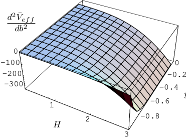
Figure 1: The behaviour of the second derivative of the radion effective potential $\bar{V}_{eff}$ is displayed as a function of $H$ (for $H^{2}>0$) and the inter-brane distance.

In the flat-brane limit, $H\rightarrow 0$, the expression inside curly brackets reduces to zero. This is also in agreement with results in the literature that consider flat-brane solutions which are saddle points (flat directions of the potential) [21, 20]. However, even in the flat limit, the presence of the scalar field allows for a non-trivial ${\cal X}$-term and the second derivative is written as

$$A^{2}\frac{d^{2}\bar{V}_{eff}}{db^{2}}=\sum_{i=1}^{2}\,\frac{4}{3\kappa^{2}_{5}}\,n_{i}^{4}\,\frac{d^{2}V_{i}}{d\phi^{2}}\,.$$ (4.17)

Again, choosing appropriately the interaction terms of the scalar field, even the flat-brane solutions à la Randall-Sundrum can be made stable.

Finally, in the case of Anti de Sitter spacetime, $H^{2}=-\tilde{H}^{2}<0$, the expression for the second derivative follows from Eq. (4.1) after making the substitutions: $H\rightarrow i\tilde{H}$ and $\sinh(3H|y_{i}|)\rightarrow i\sin(3\tilde{H}|y_{i}|)$. In that case, the expression inside curly brackets turns out to be positive-definite revealing the existence of a stabilizing force acting on the system. This is again in agreement with results presented in the literature [21]. The ${\cal X}$-term in this case has the form

$${\cal X}=\sum_{i=1}^{2}\,\frac{12\tilde{H}^{2}}{\kappa^{2}_{5}}\,\frac{y_{i}^{2}\,n_{i}^{4}}{\sin^{2}(3\tilde{H}y_{i})}\,\frac{d^{2}V_{i}}{d{\phi}^{2}}\,,$$ (4.18)

and it may act again as an extra stabilizing force if $d^{2}V_{i}/d\phi^{2}>0$. It is worth noting that, if the above inequality holds, the ${\cal X}$-term acts as a universal stabilizing force independently of the value of the effective cosmological constant on the brane.

4.2 Stability behaviour of the solutions with $V_{B}\neq 0$

We now turn to the stability analysis of the solutions derived in section 3.2, that are characterized by a non-vanishing bulk potential $V_{B}$. Changing to non-conformal coordinates, the perturbed five-dimensional line-element may be written as

$$ds^{2}=n^{2}(t,y)\,[\,-dt^{2}+a^{2}(t)\,\gamma_{ij}\,dx^{i}\,dx^{j}\,]+b^{2}(t)\,dy^{2}\,.$$ (4.19)

The above metric ansatz is similar to that used in Ref. [20], therefore, the details of the analysis that lead to the expressions of the stabilization constraints can be found there. Here, we present only the main points of our calculation that allow for the generalization of those results in the case of a non-vanishing effective cosmological constant.

For the above ansatz, the scalar curvature may be expressed as in Eq. (4.2) with the only difference, relevant to our purposes, being

$$\hat{R}^{(y)}=-\frac{1}{b^{2}}\,\biggl{(}\frac{12n^{\prime 2}}{n^{2}}+\frac{8n^{\prime\prime}}{n}\biggr{)}\,.$$ (4.20)

Substituting the expression of $\hat{R}$ in the action and performing the same conformal transformation, the effective potential finally takes the form

$$A^{2}(by_{1},by_{2})\,\bar{V}_{eff}=2\int_{by_{1}}^{by_{2}}d\xi\,n^{4}\,\biggl{(}-\frac{6}{\kappa^{2}_{5}}\,\frac{n^{\prime 2}}{n^{2}}+\frac{\phi^{\prime 2}}{2}+\Lambda_{B}+V_{B}\biggr{)}+\sum_{i=1}^{2}n_{i}^{4}\,(V_{i}+\Lambda_{i})\,,$$ (4.21)

where now

$$A(by_{1},by_{2})=\frac{2\kappa^{2}_{4}}{\kappa^{2}_{5}}\,\int_{by_{1}}^{by_{2}}d\xi\,n^{2}(\xi)\,.$$ (4.22)

The extremization constraint demands the first derivative of the effective potential, with respect to $b$, to vanish when evaluated at the background solution (3.32). Differentiating once with respect to $b$ and using the jump conditions

$$\frac{n^{\prime}_{i}}{n_{i}}=\mp\frac{\kappa_{5}^{2}}{6}\,\Bigl{[}\Lambda_{i}+V_{i}(\phi_{i})\Bigr{]}\,,\qquad\phi^{\prime}_{i}=\pm\frac{1}{2}\,\frac{\partial V_{i}(\phi)}{\partial\phi}\Biggl{|}_{y=y_{i}}\,,$$ (4.23)

for $i=1,2$, respectively, we obtain:

$$A^{2}\,\frac{d\bar{V}_{eff}}{db}=2y_{i}\,n_{i}^{4}\Biggl{[}\Lambda_{B}+V_{B}+\frac{\kappa^{2}_{5}}{6}\,(\Lambda_{i}+V_{i})^{2}-\frac{1}{8}\,\biggl{(}\frac{dV_{i}}{d\phi}\biggr{)}^{2}\Biggr{]}\Biggl{|}_{i=1}^{i=2}-2A\,\frac{dA}{db}\,\bar{V}_{eff}\Biggl{|}_{i=1}^{i=2}\,.$$ (4.24)

The expression of $dA/db$ is given, in this case, by Eq. (4.11) with $n_{i}^{3}$ replaced by $n_{i}^{2}$, while $\bar{V}_{eff}$ is still given by Eq. (4.12). Finally, we may use the relation

$$V_{B}(y_{i})=3E-\frac{3}{2}\,\phi^{\prime 2}_{i}=3E-\frac{3}{8}\,\biggl{(}\frac{dV_{i}}{d\phi}\biggr{)}^{2}\,.$$ (4.25)

If we put everything together, the extremization constraint becomes

$$A^{2}\frac{d\bar{V}_{eff}}{db}=y_{i}\,n_{i}^{4}\Biggl{[}-\frac{12}{\kappa_{5}^{2}}\frac{H^{2}}{n_{i}^{2}}+\frac{\kappa_{5}^{2}}{3}(V_{i}+\Lambda_{i})^{2}-\Bigl{(}\frac{dV_{i}}{d\phi}\Bigr{)}^{2}+2(3E+\Lambda_{B})\Biggr{]}\Biggr{|}_{i=1}^{i=2}\equiv 0\,.$$ (4.26)

We can easily check that the second equality indeed holds if we use the jump conditions (3.36)-(3.37).

After differentiating twice Eq. (4.21) with respect to $b$, we arrive at the stabilization constraint. Once again, using the jump conditions (4.23) and the equation of motion of the scalar field in the bulk (3.27), together with Eq. (3.26), we arrive at

$$A^{2}\frac{d^{2}\bar{V}_{eff}}{db^{2}} = \sum_{i=1}^{2}y_{i}^{2}n_{i}^{4}\kappa_{5}^{2}\,(V_{i}+\Lambda_{i})\Biggl{[}\frac{2\kappa_{5}^{2}}{9}\,(V_{i}+\Lambda_{i})^{2}+\frac{4}{3}\,(3E+\Lambda_{B})-\frac{3}{4}\,\biggl{(}\frac{dV_{i}}{d\phi}\biggr{)}^{2}\Biggr{]}$$ (4.27)

$$+ \frac{1}{4}\sum_{i=1}^{2}y_{i}^{2}n_{i}^{4}\,\frac{d^{2}V_{i}}{d\phi^{2}}\,\biggl{(}\frac{dV_{i}}{d\phi}\biggr{)}^{2}-2\Biggl{[}\biggl{(}\frac{dA}{db}\biggr{)}^{2}+A\frac{d^{2}A}{db^{2}}\Biggr{]}\bar{V}_{eff}\,.$$

Let us first concentrate on the case with $\omega^{2}>0$. By using the corresponding solution for the warp factor from Eq. (3.32) and the jump conditions (3.36)-(3.37), we obtain the final expression

$$A^{2}\frac{d^{2}\bar{V}_{eff}}{db^{2}}={\cal X}+\frac{\omega}{\kappa^{2}_{5}}\,\Biggl{\{}\biggl{(}\frac{12\omega^{2}}{\sinh^{2}(\omega y_{1})}-5\kappa^{2}_{5}c^{2}\Bigl{)}\,{\cal Y}+16\,\biggl{(}\kappa^{2}_{5}c^{2}-\frac{3\omega^{2}}{\sinh^{2}(\omega y_{1})}\biggl{)}\,{\cal Z}\Biggr{\}}\,,$$ (4.28)

where we have defined ${\cal X}$, ${\cal Y}$ and ${\cal Z}$ as:

$${\cal X}=\sum_{i=1}^{2}c^{2}y_{i}^{2}n_{i}^{2}\,\frac{d^{2}V_{i}}{d\phi^{2}}\,,$$ (4.29)

$${\cal Y}=\frac{y_{1}^{2}\sinh(2\omega|y_{1}|)-y_{2}^{2}\sinh(2\omega|y_{2}|)}{\sinh^{2}(\omega y_{1})}\,,$$ (4.30)

$${\cal Z}=\frac{1}{\sinh^{2}(\omega y_{1})}\,\frac{\Bigl{[}y_{2}\sinh^{2}(\omega y_{2})-y_{1}\sinh^{2}(\omega y_{1})\Bigr{]}^{2}}{2\omega(y_{1}-y_{2})+\sinh(2\omega|y_{1}|)-\sinh(2\omega|y_{2}|)}\,.$$ (4.31)

In Eq. (4.28), the constraint relating $\chi$ and $\omega$ that appears in Eq. (3.32), may be rewritten as

$$H^{2}=\frac{\omega^{2}}{\sinh^{2}(\omega y_{1})}-\frac{\kappa^{2}_{5}c^{2}}{3}\,,$$ (4.32)

and has been used to eliminate one parameter from the expression of the second derivative. The value of this quantity still depends on $\omega$ and $c^{2}$, that parametrize the size of the bulk quantities, $\Lambda_{B}$ and ${\cal L}_{B}(\phi)$, and the inter-brane distance, parametrized by the values of $y_{i}$. For simplicity, we may fix the locations of the two branes at $y_{i}=-1$ and $y_{2}=-0.5$, while the singularity lies at $y=0$. As was pointed out in section 3.2, the parameter $c^{2}$ may take both positive and negative values; this may lead to different behaviours of the background solution under time-dependent perturbations, as we will now see. In Figure 2, we display the value of the second derivative of the effective potential - the expression inside curly brackets in Eq. (4.28) - for both signs of $c^{2}$ and we comment on the results below:

     

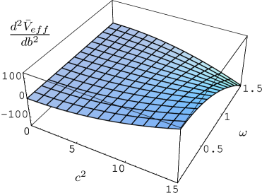
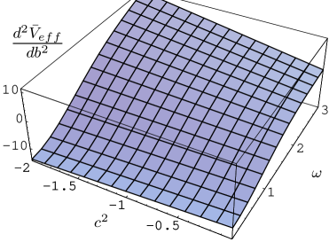
Figure 2: The two plots depict the second derivative of the radion effective potential $\bar{V}_{eff}$ as a function of $\omega$ (with $\omega^{2}>0$) and for positive and negative values of $c^{2}$, respectively.

• $c^{2}>0$: The second derivative assumes positive values for large enough $c^{2}$ but small $\omega$. In other words, the background solution is more stable when the kinetic term of the scalar field is larger and the bulk cosmological constant is smaller. Eq. (4.32) then reveals that this particular regime of parameters corresponds to solutions with a negative cosmological constant on the brane.

• $c^{2}<0$: Positive values for the second derivative can be achieved for large enough values of both $c^{2}$ and $\omega$. In this case, the effective cosmological constant on the brane is positive by definition and therefore physically interesting, stable solutions may emerge in this case.

It is worth noting that, in the above cases, we obtain positive sign for the second derivative of the radion potential even if we assume that $d^{2}V_{i}/d\phi^{2}=0$, contrary to what happened in section 4.1. An extra stabilizing force may arise, for $c^{2}>0$ or $c^{2}<0$, if $d^{2}V_{i}/d\phi^{2}>0$ or $d^{2}V_{i}/d\phi^{2}<0$, respectively. Let us finally note that in the parameter regimes where the solution is clearly stable or unstable, the sole effect of the inter-brane distance is to change the magnitude of the radion mass squared: larger inter-brane distances imply larger (in absolute value) second derivatives. In the intermediate regime, where the solutions struggle between stability and instability, stable solutions may arise when the second brane is located closer to the first one and away from the singularity.

In the special case of $\omega=0$, the expression of the second derivative of the effective potential may be obtained from Eq. (4.28) by taking the limit $\omega\rightarrow 0$. Then, we find

$$A^{2}\frac{d^{2}\bar{V}_{eff}}{db^{2}}=\sum_{i=1}^{2}\frac{c^{2}y_{i}^{4}}{y_{1}^{2}}\,\frac{d^{2}V_{i}}{d\phi^{2}}+\frac{2}{\kappa^{2}_{5}y_{1}^{2}}\,\Bigl{(}\kappa_{5}^{2}c^{2}-{6}{\chi^{2}}\Bigr{)}\,(|y_{1}|^{3}-|y_{2}|^{3})\,.$$ (4.33)

The second term has a positive value only if $\kappa^{2}_{5}c^{2}>6\chi^{2}>0$. In this case, the first term also contributes positively to the second derivative if $d^{2}V_{i}/d\phi^{2}>0$. In this case, stable solutions with a negative cosmological constant on the brane arise.

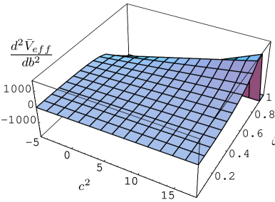
Figure 3: The plot depicts the second derivative of the radion effective potential $\bar{V}_{eff}$ as a function of the $\tilde{\omega}$ and $c^{2}$ parameters.

Finally, we turn to the case with $\omega^{2}<0$. The expression of the second derivative may again be obtained from Eq. (4.28) by making the substitutions: $\omega\rightarrow i\tilde{\omega}$ and $\sinh(\omega y_{i})\rightarrow i\sin(\tilde{\omega}y_{i})$. Given the new form of the warp factor, the two branes should now be located between the two singularities at $y=0$ and $\tilde{\omega}y=-\pi$. We therefore set $y_{1}=-\pi$ and we allow $\tilde{\omega}$ to vary in the interval (0,1) - $y_{2}$ is placed in between, with the size of the inter-brane distance having no effect on the behaviour of the second derivative. In Figure 3, we display the value of the second derivative as a function of $c^{2}$ and $\tilde{\omega}$. We may easily see that stable solutions arise for large enough, positive values of $c^{2}$, with the solutions becoming more and more stable as the value of $\tilde{\omega}$ increases. An unstable regime appears when $\tilde{\omega}\rightarrow 1$, which is equivalent to placing the first brane very close to the singularity at $\tilde{\omega}y=-\pi$. By using Eq. (4.32), we may see that the stable regime corresponds to solutions with a negative cosmological constant on the brane.

5 Conclusions

There has been a lot of work related to the stabilization of the radion field that parametrizes the size of the extra dimension in the context of brane-world models. Most work has focused on the derivation of solutions with a constant radion field, i.e. a static extra dimension, with only a few papers investigating whether these solutions correspond to a true minimum of the radion effective potential. In this paper, we presented two new, brane-world solutions arising in the presence of a bulk scalar field, and studied their stability under time-dependent perturbations of the radion field demonstrating the existence of phenomenologically interesting, stable solutions with a positive cosmological constant on the brane.

For our analysis, we used a factorizable ansatz for the line-element along the brane. Under the assumption that the total energy of each brane is the sum of a constant brane tension and the interaction term of a time-independent, bulk scalar field, the factorization of the 3D scale factor was shown to be directly related to the stabilization of the extra dimension. This relation holds both on and off the brane, as one can see by using the scale factor jump conditions and the off-diagonal component of Einstein’s equations, respectively.

The first class of solutions presented here corresponds to a vanishing bulk potential for the scalar field and a vanishing bulk cosmological constant. Surprisingly enough, brane-world solutions with non-trivial warping along the extra dimension did emerge, with the ‘warping’ parameter being the expansion rate on the brane. These configurations accept a variety of time-dependent solutions for the scale factor on the brane, with flat ($k=0$) or curved ($k=\pm 1$) 3D spacetime and a zero, positive or negative effective cosmological constant. All of the above solutions are characterized by the presence of a bulk curvature singularity, which inevitably leads to the introduction of a second brane in the model. One can show that the jump conditions, imposed on the warp factor and the scalar field, lead to the fixing of the inter-brane distance, in terms of the fundamental parameters of the theory, and that the conventional Friedmann equation on the brane is successfully recovered.

In the second class of solutions that we derived, the presence of a non-trivial bulk potential and a bulk cosmological constant was restored. In this case, the warping of the 5D metric was governed by the bulk cosmological constant shifted by a constant quantity given in terms of the kinetic and potential energy of the bulk field. The same variety of cosmological solutions on the brane emerge here as well. The sign of the kinetic term of the scalar field reveals its nature (normal or tachyonic) and affects the behaviour of the bulk potential: a normal kinetic term leads to a potential which is unbounded from below, near the bulk singularity, whereas a tachyonic kinetic term leads to an infinitely-high potential barrier that may be used to shield the singularity in single-brane configurations. Here, we introduced a second brane in order to do so, and we demonstrated that, as in the first case, the inter-brane distance is fixed and the form of the Friedmann equation on the brane is recovered.

In the second part of our paper, we investigated the stability of our solutions under small, time-dependent perturbations of the radion field. We derived the extremization constraints for both types of solutions and demonstrated that, as expected, they correspond to extrema of the radion effective potential. The stabilization constraints were also derived. These revealed the stability behaviour of the solutions and the type of extrema to which they correspond, either minima or maxima. In the first class of solutions, brane configurations with positive, zero or negative effective cosmological constant were studied and it was shown that, in the absence of a scalar field potential, those solutions come out to be local maxima, saddle points or minima of the radion effective potential, respectively, in agreement with the literature. However, in our case, the presence of an extra term, involving second derivatives of the interaction terms of the scalar field on the branes, acts as a universal stabilizing force, independent of the sign of the cosmological constant on the brane, as long as the second derivatives are positive. In this way, solutions with a positive cosmological constant on the brane may become stable, saddle-point solutions à la Randall-Sundrum may turn to true minima, and AdS-type solutions on the brane may be further stabilized. The results for the second class of solutions found in this paper are even more interesting: the aforementioned term with the derivatives of the interaction terms may still act as an extra stabilizing force - upon appropriate choice of the sign of the second derivatives - nevertheless, stable solutions can arise even in the case where this term is zero. The parameter regimes that correspond to stable solutions are determined by the values of the bulk cosmological constant and the kinetic term of the scalar field. It is worth noting that the sign of the latter quantity also defines the sign of the effective cosmological constant of the stable solution: a normal (positive) kinetic term gives rise to solutions with negative cosmological constant, while a tachyonic (negative) one leads to a positive effective cosmological constant.

We may, therefore, conclude that the introduction of a bulk scalar field, in a brane-world model, may successfully lead to a variety of stable solutions, but more importantly, it may lead to cosmologically interesting, stable solutions with a positive effective cosmological constant - a type of solutions that has been difficult to derive up to now.

References

- [1] I. Antoniadis, Phys. Lett. B 246, 377 (1990); N. Arkani-Hamed, S. Dimopoulos and G. Dvali, Phys. Lett. B 429, 263 (1998) [hep-ph/9803315]; I. Antoniadis, N. Arkani-Hamed, S. Dimopoulos and G. Dvali, Phys. Lett. B 436, 257 (1998) [hep-ph/9804398].
- [2] L. Randall and R. Sundrum, Phys. Rev. Lett. 83, 3370 (1999) [hep-ph/9905221]; Phys. Rev. Lett. 83, 4690 (1999) [hep-th/9906064].
- [3] J. Lykken and L. Randall, JHEP 0006, 014 (2000) [hep-th/9908076]; J. Cline, C. Grojean and G. Servant, Phys. Lett. B 472, 302 (2000) [hep-ph/9909496]; A. G. Cohen and D. B. Kaplan, Phys. Lett. B 470, 52 (1999) [hep-th/9910132]; Z. Chacko and A. E. Nelson, Phys. Rev. D 62, 085006 (2000) [hep-th/9912186]; M. Chaichian and A.B. Kobakhidze, Phys. Lett. B 478, 299 (2000) [hep-th/9912193]; N. Arkani-Hamed, L. J. Hall, D. R. Smith and N. Weiner, Phys. Rev. D 62, 105002 (2000) [hep-ph/9912453]; P. Kanti, K. A. Olive and M. Pospelov, Phys. Rev. D 62, 126004 (2000) [hep-ph/0005146].
- [4] N. Arkani-Hamed, S. Dimopoulos, N. Kaloper and J. March-Russell, Nucl. Phys. B 567, 189 (2000) [hep-ph/9903224]; N. Arkani-Hamed, S. Dimopoulos and J. March-Russell, Phys. Rev. D 63, 064020 (2001) [hep-th/9809124]; P. Kanti and K. A. Olive, Phys. Rev. D 60, 043502 (1999) [hep-ph/9903524]; Phys. Lett. B 464, 192 (1999) [hep-ph/9906331]; N. Arkani-Hamed, S. Dimopoulos, G. R. Dvali and N. Kaloper, JHEP 0012, 010 (2000) [hep-ph/9911386].
- [5] A. Lukas, B.A. Ovrut, K.S. Stelle and D. Waldram, Phys. Rev. D 59, 086001 (1999) [hep-th/9803235]; A. Lukas, B.A. Ovrut and D. Waldram, Phys. Rev. D 60, 086001 (1999) [hep-th/9806022]; D 61, 023506 (2000) [hep-th/9902071].
- [6] N. Kaloper and A. Linde, Phys. Rev. D 59, 101303 (1999) [hep-th/9811141].
- [7] P. Binétruy, C. Deffayet and D. Langlois, Nucl. Phys. B 565 (2000) 269 [hep-th/9905012].
- [8] T. Nihei, Phys. Lett. B 465, 81 (1999) [hep-ph/9905487]; N. Kaloper, Phys. Rev. D 60, 123506 (1999) [hep-th/9905210].
- [9] C. Csáki, M. Graesser, C. Kolda and J. Terning, Phys. Lett. B 462, 34 (1999) [hep-ph/9906513]; J.M. Cline, C. Grojean and G. Servant, Phys. Rev. Lett. 83, 4245 (1999) [arXiv:hep-ph/9906523].
- [10] D. J. Chung and K. Freese, Phys. Rev. D 61, 023511 (2000) [hep-ph/9906542]; A. Brandhuber and K. Sfetsos, JHEP 9910, 013 (1999) [hep-th/9908116]; H. B. Kim and H. D. Kim, Phys. Rev. D 61, 064003 (2000) [hep-th/9909053]; U. Ellwanger, Phys. Lett. B 473, 233 (2000) [hep-th/9909103], E. E. Flanagan, S. H. Tye and I. Wasserman, Phys. Rev. D 62, 044039 (2000) [hep-ph/9910498]; C. Schmidhuber, Nucl. Phys. B 580, 140 (2000) [hep-th/9912156]; H. B. Kim, Phys. Lett. B 478, 285 (2000) [hep-th/0001209];
- [11] I. I. Kogan, S. Mouslopoulos, A. Papazoglou, G. G. Ross and J. Santiago, Nucl. Phys. B 584, 313 (2000) [hep-ph/9912552]; I. I. Kogan and G. G. Ross, Phys. Lett. B 485, 255 (2000) [hep-th/0003074]. I. I. Kogan, S. Mouslopoulos, A. Papazoglou and G. G. Ross, Nucl. Phys. B 595, 225 (2001) [hep-th/0006030]; I. I. Kogan, S. Mouslopoulos and A. Papazoglou, Phys. Lett. B 501, 140 (2001) [hep-th/0011141].
- [12] C. Barcelo and M. Visser, Phys. Lett. B 482, 183 (2000) [hep-th/0004056]; J. Lesgourgues, S. Pastor, M. Peloso and L. Sorbo, Phys. Lett. B 489, 411 (2000) [hep-ph/0004086]; H. Stoica, S. H. Tye and I. Wasserman, Phys. Lett. B 482, 205 (2000) [hep-th/0004126]; J. E. Kim and B. Kyae, Phys. Lett. B 486, 165 (2000) [hep-th/0005139]; K. Enqvist, E. Keski-Vakkuri and S. Rasanen, Phys. Rev. D 64, 044017 (2001) [hep-th/0007254];
- [13] P. Kanti, I. Kogan, K.A. Olive and M. Pospelov, Phys. Lett. B 468, 31 (1999) [hep-ph/9909481].
- [14] C. Csáki, M. Graesser, L. Randall, and J. Terning, Phys. Rev. D 62, 045015 (2000) [hep-ph/9911406].
- [15] P. Kanti, I. Kogan, K.A. Olive and M. Pospelov, Phys. Rev. D 61, 106004 (2000) [hep-ph/9912266].
- [16] O. DeWolfe, D. Z. Freedman, S. S. Gubser and A. Karch, Phys. Rev. D 62, 046008 (2000) [hep-th/9909134]; N. Arkani-Hamed, S. Dimopoulos, N. Kaloper and R. Sundrum, Phys. Lett. B 480, 193 (2000) [hep-th/0001197]; S. Kachru, M. B. Schulz and E. Silverstein, Phys. Rev. D 62, 045021 (2000) [hep-th/0001206]; B. Grinstein, D. R. Nolte and W. Skiba, Phys. Rev. D 62, 086006 (2000) [hep-th/0005001]; Z. Kakushadze, Nucl. Phys. B 589, 75 (2000) [hep-th/0005217]; S. Forste, Z. Lalak, S. Lavignac and H. P. Nilles, JHEP 0009, 034 (2000) [hep-th/0006139]; C. Barcelo and M. Visser, Phys. Rev. D 63, 024004 (2001) [gr-qc/0008008]; A. Mennim and R. A. Battye, Class. Quant. Grav. 18, 2171 (2001) [hep-th/0008192]; A. Kehagias and K. Tamvakis, hep-th/0011006. N. Sago, Y. Himemoto and M. Sasaki, Phys. Rev. D 65, 024014 (2002) [gr-qc/0104033]; E. E. Flanagan, S. H. Tye and I. Wasserman, Phys. Lett. B 522, 155 (2001) [hep-th/0110070].
- [17] P. Kanti, K. A. Olive and M. Pospelov, Phys. Lett. B 481, 386 (2000) [hep-ph/0002229].
- [18] W. D. Goldberger and M. B. Wise, Phys. Rev. D 60, 107505 (1999) [hep-ph/9907218]; Phys. Rev. Lett. 83, 4922 (1999) [hep-ph/9907447].
- [19] T. Tanaka and X. Montes, Nucl. Phys. B 582, 259 (2000) [hep-th/0001092]; D. Choudhury, D. P. Jatkar, U. Mahanta and S. Sur, JHEP 0009, 021 (2000) [hep-ph/0004233]; J. M. Cline and H. Firouzjahi, Phys. Rev. D 64, 023505 (2001) [hep-ph/0005235]; V. D. Barger, T. Han, T. Li, J. D. Lykken and D. Marfatia, Phys. Lett. B 488, 97 (2000) [hep-ph/0006275]; P. Binetruy, J. M. Cline and C. Grojean, Phys. Lett. B 489, 403 (2000) [hep-th/0007029]; C. Csaki, M. L. Graesser and G. D. Kribs, Phys. Rev. D 63, 065002 (2001) [hep-th/0008151]; J. M. Cline and H. Firouzjahi, Phys. Lett. B 495, 271 (2000) [hep-th/0008185]; J. Garriga, O. Pujolas and T. Tanaka, Nucl. Phys. B 605, 192 (2001) [hep-th/0004109]. R. Hofmann, P. Kanti and M. Pospelov, Phys. Rev. D 63, 124020 (2001) [hep-ph/0012213].
- [20] P. Kanti, K. A. Olive and M. Pospelov, Phys. Lett. B 538, 146 (2002) [hep-ph/0204202].
- [21] U. Gen and M. Sasaki, Prog. Theor. Phys. 105, 591 (2001) [gr-qc/0011078]; P. Binetruy, C. Deffayet and D. Langlois, Nucl. Phys. B 615, 219 (2001) [hep-th/0101234]; Z. Chacko and P. J. Fox, Phys. Rev. D 64, 024015 (2001) [hep-th/0102023].
- [22] W. Israel, Nuovo. Cim. B44,1 (1966); Erratum ibid B48, 463 (1967).