IFIC/02-39, FTUV/02-0903

Charm and bottom quark masses from QCD moment sum rules

Abstract

In this work the charm and bottom quark masses are determined from QCD moment sum rules for the charmonium and upsilon systems. In our analysis we include both the results from non-relativistic QCD and perturbation theory at next-next-to-leading order. For the pole masses we obtain $M_{c}=1.75\pm 0.15$ GeV and $M_{b}=4.98\pm 0.125$ GeV. Using the potential-subtracted mass in intermediate steps of the calculation the ${\overline{\rm MS}}$-masses are determined to $m_{c}(m_{c})=1.19\pm 0.11$ GeV and $m_{b}(m_{b})=4.24\pm 0.10$ GeV.

1 Introduction

An important task within modern particle phenomenology consists in the determination of the quark masses, being fundamental parameters of the Standard Model. In the past, QCD moment sum rule analyses have been successfully applied for extracting the charm and bottom quark masses from experimental data on the charmonium and bottomium systems respectively [1, 2, 3]. The basic quantity in these investigations is the vacuum polarisation function $\Pi(q^{2})$:

$$\Pi_{\mu\nu}(q^{2}) = i\int d^{4}x\ e^{iqx}\,\langle T\{j_{\mu}(x)j_{\nu}^{\dagger}(0)\}\rangle$$ (1)

$$= (q_{\mu}q_{\nu}-g_{\mu\nu}q^{2})\,\Pi(q^{2})\,,$$

where the relevant vector current is represented either by the charm $j_{\mu}^{c}(x)=(\bar{c}\gamma_{\mu}c)(x)$ or the bottom current $j_{\mu}^{b}(x)=(\bar{b}\gamma_{\mu}b)(x)$. Via the optical theorem, the experimental cross section $\sigma(e^{+}e^{-}\to c\bar{c},b\bar{b})$ is related to the imaginary part of $\Pi(s)$:

$$R(s)=\frac{1}{Q_{c,b}^{2}}\,\frac{\sigma(e^{+}e^{-}\to c\bar{c},b\bar{b})}{\sigma(e^{+}e^{-}\to\mu^{+}\mu^{-})}=12\pi\,\mbox{\rm Im}\,\Pi(s)\,.$$

Usually, moments of the vacuum polarisation are defined by taking derivatives of the correlator at $s=0$. However, in this work we allow for an arbitrary evaluation point $s=-4m^{2}\xi$ to define the dimensionless moments [4]:

$${\cal M}_{n}(\xi) = \frac{12\pi^{2}}{n!}\left(4m^{2}\frac{d}{ds}\right)^{n}\Pi(s)\bigg{|}_{s=-4m^{2}\xi}$$ (2)

$$= 2\int\limits_{0}^{1}\!dv\,\frac{v(1-v^{2})^{n-1}R(v)}{(1+\xi(1-v^{2}))^{n+1}}\,,$$

where $v=\sqrt{1-4m^{2}/s}$ is the velocity of the heavy quark. The parameter $\xi$ encodes much information about the system. By taking $\xi$ larger the evaluation point moves further away from the threshold region. Consequently, the theoretical expansions show a better convergence, but at the same time the sensitivity on the mass is reduced. The moments can either be calculated theoretically, including Coulomb resummation, perturbation theory and nonperturbative contributions, or be obtained from experiment. In this way one can relate the heavy quark masses to the hadronic properties of the quark-antiquark systems.

A characteristic feature of these heavy-heavy bound state systems is the Coulomb-like form of the potential. Developing the quantum mechanical sum rules for Coulomb systems, in [4] it has been shown that the application of fixed-order perturbation theory in such systems results in unstable predictions for the masses. To obtain a stable sum rule it is necessary to incorporate the threshold behaviour which can be calculated in the framework of non-relativistic QCD (NRQCD).

A natural choice for the mass in eq. (2) is the pole mass $M$. First we will employ the pole mass scheme to extract the pole masses. However, as the pole masses suffer from renormalon ambiguities [5], we shall then use the potential-subtracted (PS-) mass $m_{PS}$ [6] to extract the ${\rm{\overline{\rm MS}}}$-masses.

2 Coulomb resummation

The theory of NRQCD provides a consistent framework to treat the problem of heavy quark-antiquark production close to threshold. The contributions can be described by a nonrelativistic Schrödinger equation and systematically calculated in time-independent perturbation theory (TIPT). The correlator is expressed in terms of a Green’s function $G(k)=G(0,0,k)$ [7, 8, 9]:

$$\Pi(s)=\frac{N_{c}}{2M^{2}}\left(C_{h}(\alpha_{s})G(k)+\frac{4k^{2}}{3M^{2}}G_{C}(k)\right)\,,$$ (3)

where $k=\sqrt{M^{2}-s/4}$ and $M$ represents the pole mass. The constant $C_{h}(\alpha_{s})$ is a perturbative coefficient needed for the matching between the full and the nonrelativistic theory and naturally depends on the hard scale.

To calculate the moments from the Green’s function we will directly perform the derivatives at $s=-4M^{2}\xi$ according to eq. (2). Since the Green’s function is known analytically [9] as a function of $k=k(s)$, this can be done numerically. In this way we take advantage of the fact that the perturbative expansion parameter depends on the evaluation point. In addition, we can extract the spectral density above threshold by taking the imaginary part of the Green’s function [4, 10].

The moments depend on the three scales $\mu_{soft}$, $\mu_{fac}$ and $\mu_{hard}$, the soft, factorisation and hard scale respectively. The residual dependence on these scales will turn out to give the dominant error in the determination of the masses. The large corrections are partly due to the definition of the pole mass. These contributions can be reduced by using an intermediate mass definition. In this analysis we will use the potential-subtracted (PS) mass [6] where the potential below a separation scale $\mu_{sep}$ is subtracted. This mass definition leads to an improved scale dependence and a more precise determination of the ${\rm{\overline{\rm MS}}}$-masses.

3 Perturbative expansion

The perturbative spectral function $R^{Pert}(s)$ can be expanded in powers of the strong coupling constant,

$$R^{Pt}(s)=R^{(0)}(s)+\frac{\alpha_{s}}{\pi}\,R^{(1)}(s)+\frac{\alpha_{s}^{2}}{\pi^{2}}\,R^{(2)}(s)+\ldots$$

From this expression the corresponding moments ${\cal M}_{n}$ can be calculated via the integral of eq. (2). The first two terms are known analytically and can for example be found in ref. [11]. $R^{(2)}(s)$ is still not fully known analytically. We employ a method based on Padé-approximants to construct the spectral density in the full energy range [12, 13]. It uses available information around $q^{2}=0$, at threshold and in the high energy region. It has the advantage that it gives a good description until relatively close to threshold, the region on which the quark masses are most sensitive.

4 Condensate contributions

The non-perturbative effects on the vacuum correlator are parametrised by the condensates. The leading correction is the gluon condensate contribution which is known up to next-to-leading order [14]. Furthermore, in [15, 16] the dimension 6 and 8 condensates have been calculated. From the numerical analysis it turns out that the absolute contribution of the condensates to the moments is negligible for the bottomium and of little influence for the charmonium. The relative suppression of the gluon condensate to former charmonium analyses is due to three reasons: First, the absolute value of the theoretical moments increases from the Coulomb resummation. Then we evaluate the moments at larger $\xi$ and smaller $n$ where the nonperturbative contributions are relatively small. Finally, since we obtain a larger pole mass than former analyses, the condensates, starting with a power of $1/M^{4}$, are suppressed further.

5 Phenomenological spectral function

Experimentally, the six lowest lying $\psi-$ and $\Upsilon-$resonances have been observed. Furthermore, recent measurements of BES [17] in the charmonium region have improved the cross section between 3.7 and 4.8 GeV. Since the widths of the poles are very small compared to the masses, the narrow-width approximation provides an excellent description of these states. To model the contributions above the 6th resonance in the bottomium system we use the assumption of quark-hadron-duality and integrate the theoretical spectral density above $\sqrt{s_{0}}=11.0\pm 0.2$ GeV. In the charmonium system we include the two lowest resonances, the BES data and the theoretical spectral density above 4.8 GeV.

6 Numerical analysis

The theoretical part of the correlator contains the poles of the Green’s function, the spectral density above threshold and the condensates. For high velocities the spectral density is well described by the perturbative expansion whereas the resummed spectral density gives a good description for low values of $v$. Therefore we construct a theoretical spectral density in the full energy range which includes the essential information in both regions of $v$. For a more detailed discussion the reader is referred to [4]. Now we discuss the most important points in the numerical analysis of the bottomium and charmonium systems respectively.

6.1 Bottom mass

First we discuss the values of $\xi$ and $n$. Since the bottom quark is relatively heavy, even for $\xi=0$ the nonrelativistic and perturbative expansions converge reasonably well. Nevertheless, the contributions from the poles of the Green’s function still dominate the theoretical part. To reduce their influence and to spread the theoretical contributions more equally among the poles, the resummed spectral density and the perturbative spectral density we must choose a higher $\xi$. However, for $\xi>1$ the moments loose sensitivity on the mass and the error from the input parameters increases. Therefore we use a central value of $\xi=0.5$ and vary $\xi$ between $0\leq\xi\leq 1$. Since the relevant scale for the evaluation point is the lowest bound state energy, values of $\xi=0,0.5$ or 1 already correspond to well separated evaluation points. For $n$ we use a range of $5\leq n\leq 10$ where the theoretical expansion and the phenomenological uncertainty are under control.

As central values for our scales we have selected $\mu_{soft}=2.5$ GeV, $\mu_{fac}=3.5$ GeV and $\mu_{hard}=5.0$ GeV. For the error estimate we vary these values between $2.0\ \mbox{GeV}\leq\mu_{soft}\leq 3.5\ \mbox{GeV}$, $2.0\ \mbox{GeV}\leq\mu_{fac\ }\leq 5.0\ \mbox{GeV}$ and $2.5\ \mbox{GeV}\leq\mu_{hard}\leq 10.0\ \mbox{GeV}$. For the separation scale $\mu_{sep}$ which appears as additional parameter in the definition of the PS-mass we employ a value of $\mu_{sep}=2.0\pm 1.0$ GeV.

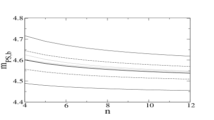
Figure 1: Thick solid line: central PS-mass; thin solid lines: $m_{PS,b}$ for $\mu_{soft}=2.0$ and 3.5 GeV; dashed lines: $m_{PS,b}$ for $\mu_{fac}=2.0$ and 5.0 GeV; dotted lines: $m_{PS,b}$ for $\mu_{hard}=2.5$ and 10.0 GeV.

The analysis is performed independently in the pole- and PS-scheme. In figure 1 we have plotted the PS-mass as a function of $n$ and the influence of the scale variations. The largest contribution to the error comes from the soft scale. Adding the errors from all input parameters quadratically, our final results for the masses are

$$M_{b} = 4.984\pm 0.125\ \mbox{GeV}\,,$$

$$m_{PS,b}(2.0\ \mbox{GeV}) = 4.561\pm 0.112\ \mbox{GeV}\,,$$

$$m_{b}(m_{b}) = 4.241\pm 0.098\ \mbox{GeV}\,.$$ (4)

6.2 Charm mass

As in the bottom case we use $\xi=0.5$. At this value the pole contributions still represent the dominant part. In principle one would like to choose a higher value where the theoretical expansions converge better. However, the contribution from the theoretical poles varies significantly with the scales; for $\xi\mathrel{\hbox to0.0pt{\lower 4.0pt\hbox{\hskip 1.0pt$\sim$}\hss}\raise 1.0pt\hbox{$>$}}1$ the mass depends too strongly on these variations. Thus we again use a range of $0\leq\xi\leq 1$. Since the perturbative expansions converge more slowly than for the upsilon we restrict the analysis to smaller values of $4\leq n\leq 7$. As central values for our scales we have selected $\mu_{fac}=1.45$ GeV, $\mu_{hard}=1.75$ GeV and values of $\mu_{soft}=1.2$ GeV and $\mu_{soft}=1.1$ GeV in the pole- and PS-schemes respectively. For the error estimate we have varied the scales between $1.4\ \mbox{\rm GeV}\leq\mu_{hard}\leq 2.5\ \mbox{\rm GeV}$, $1.2\ \mbox{\rm GeV}\leq\mu_{fac}\leq 1.65\ \mbox{\rm GeV}$ and $1.1(1.0)\ \mbox{\rm GeV}\leq\mu_{soft}\leq 1.35(1.25)\ \mbox{\rm GeV}$. For the separation scale we choose $\mu_{sep}=1.0\pm 0.2\ \mbox{\rm GeV}$.

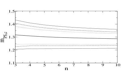
Figure 2: Thick solid line: central PS-mass; thin solid lines: $m_{PS,c}$ for $\mu_{soft}=1.0$ and 1.25 GeV; dashed lines: $m_{PS,c}$ for $\mu_{fac}=1.2$ and 1.65 GeV; dotted lines: $m_{PS,c}$ for $\mu_{hard}=1.4$ and 2.5 GeV.

In figure 2 we have plotted the PS-mass and the corresponding error from the scales. Finally we obtain the masses:

$$M_{c} = 1.754\pm 0.147\ \mbox{GeV}\,,$$

$$m_{PS,c}(1.0\ \mbox{GeV}) = 1.300\pm 0.124\ \mbox{GeV}\,,$$

$$m_{c}(m_{c}) = 1.188\pm 0.106\ \mbox{GeV}\,.$$ (5)

7 Conclusions

The method of QCD sum rules is a very powerful tool to extract the masses since - by the choice of $n$ and $\xi$ - it can react very sensitive to threshold. Thus, large theoretical uncertainties only lead to a relatively small shift in the masses. We have tried to develop a consistent framework to describe the physics of the relevant energy region. The masses show a stable behaviour over a large range of $n$ and the dominant uncertainties originate from the threshold expansion of NRQCD.

Acknowledgements

I would like to thank S. Narison for the invitation to this pleasant and interesting conference. This work has been supported in part by TMR, EC contract No. ERB FMRX-CT98-0169, by MCYT (Spain) under grant FPA2001-3031, and by ERDF funds from the European Commission. I thank the Deutsche Forschungsgemeinschaft for financial support.

References

- [1] M.A. Shifman, A.I. Vainshtein and V.I. Zakharov, Nucl. Phys. B 147 (1979) 385, Nucl. Phys. B 147 (1979) 448.
- [2] L.J. Reinders, H. Rubinstein and S. Yazaki, Phys. Rep. 127 (1985) 1.
- [3] S. Narison, QCD Spectral Sum Rules, World Scientific (1989).
- [4] M. Eidemüller, hep-ph/0207237
- [5] M. Beneke, Phys. Rep. 317 (1999) 1.
- [6] M. Beneke, Phys. Lett. B 434 (1998) 115.
- [7] M.J. Strassler and M.E. Peskin, Phys. Rev. D 43 (1991) 1500.
- [8] A.H. Hoang, Phys. Rev. D 58 (1998) 114023.
- [9] A.A. Penin and A.A. Pivovarov, Nucl. Phys. B 549 (1999) 217.
- [10] M. Eidemüller and M. Jamin, Phys. Lett. B 498 (2001) 203.
- [11] M. Jamin and A. Pich, Nucl. Phys. B 507 (1997) 334.
- [12] K.G. Chetyrkin, J.H. Kühn and M. Steinhauser, Nucl. Phys. B 482 (1996) 213.
- [13] K.G. Chetyrkin, J.H. Kühn and M. Steinhauser, Nucl. Phys. B 505 (1997) 40.
- [14] D.J. Broadhurst et al., Phys. Lett. B 329 (1994) 103.
- [15] S.N. Nikolaev and A.V. Radyushkin, Nucl. Phys. B 213 (1983) 285.
- [16] S.N. Nikolaev and A.V. Radyushkin, Phys. Lett. B 124 (1983) 243.
- [17] J.Z. Bai et al. (BES Collaboration), Phys. Rev. Lett. 88 (2002) 101802.