Abstract

In the $SU(6)\times SU(2)_{R}$ string-inspired model, we evolve the couplings and the masses down from the string scale $M_{S}$ using the renormalization group equations and minimize the effective potential. This model has the flavor symmetry including the binary dihedral group $\tilde{D}_{4}$. We show that the scalar mass squared of the gauge non-singlet matter field possibly goes negative slightly below the string scale. As a consequence, the precocious radiative breaking of the gauge symmetry down to the standard model gauge group can occur. In the present model, the large Yukawa coupling which plays an important role in the symmetry breaking is identical with the colored Higgs coupling related to the longevity of the proton.

1 Introduction

In the minimal supersymmetric standard model(MSSM), it is well-known that the spontaneous breaking of the gauge symmetry $SU(2)_{L}\times U(1)_{Y}\rightarrow U(1)_{em}$ is caused around the electroweak scale by the radiative effect due to the large top Yukawa coupling.[1] On the other hand, in many supersymmetric GUT models, it is assumed that by taking the wine-bottle type of the Higgs potential by hand, the spontaneous breaking of a large gauge symmetry such as $SU(5)$ or $SO(10)$ takes place via Higgs mechanism at high energies around ${\cal O}(10^{16}{\rm GeV})$. In order to clarify whether or not the spontaneous breaking of the large gauge symmetry occurs at such a large energy scale, we need to address the underlying string theory which yields the GUT-type models. The radiative breaking of the large gauge symmetry occurs if the mass squared of a gauge non-singlet scalar field goes negative precociously as one evolves down from the string scale. Then it is of importance to study whether or not the radiative effect due to the large Yukawa couplings resulting from the underlying theory causes the scalar mass squared to be driven negative at a large energy scale. In the extra $U(1)^{2}$ string-inspired model it has been already found that the radiative effect due to the large Yukawa couplings possibly breaks down one of the extra $U(1)$ gauge symmetries around ${\cal O}(10^{15}{\rm GeV})$.[2]

In this paper we consider the $SU(6)\times SU(2)_{R}$ string-inspired model, which contains many phenomenologically attractive features.[3, 4, 5, 6, 7, 8, 9] In this model we evolve couplings and masses down from the string scale $M_{S}$ using the renormalization group(RG) equations and minimize the effective potential. The purpose of this paper is to explore whether the gauge symmetry breaking occurs or not at very large energy scale. Studying the RG evolution from the string scale $M_{S}$, we show that the scalar mass squared of the gauge non-singlet matter field possibly goes negative slightly below the string scale. This implies that the precocious breaking of the gauge symmetry $SU(6)\times SU(2)_{R}$ can occur due to the radiative effect. In this model the large Yukawa coupling which plays an important role in the symmetry breaking is identical with the colored Higgs coupling related to the longevity of the proton. This symmetry breaking triggers off the subsequent symmetry breaking.[10] Thus we obtain the sequential symmetry breaking

$$SU(6)\times SU(2)_{R}\longrightarrow SU(4)_{PS}\times SU(2)_{L}\times SU(2)_{R}\longrightarrow G_{SM},$$

where $SU(4)_{PS}$ and $G_{SM}$ represent the Pati-Salam $SU(4)$[11] and the standard model gauge group, respectively.

In the framework of the string theory we are prohibited from adding extra matter fields by hand. In the effective theory from string, the matter contents and the Lagrangian are strongly constrained due to the topological and the symmetrical structure of the compact space. This situation is in sharp contrast to the conventional GUT-type models. For instance, in the perturbative heterotic string we have no adjoint or higher representation matter(Higgs) fields. Also, in the context of the brane picture, matter fields belong to the bi-fundamental or the anti-symmetric representations under the gauge group such as $SU(M)\times SU(N)$. In the present model, under $SU(6)\times SU(2)_{R}$, gauge non-singlet matter fields consist of $({\bf 15},{\bf 1})$, $({\bf 6^{*}},{\bf 2})$ and their conjugates. Within the rigid framework we have to find out the path from the string scale physics to the low-energy physics. ¿From this point of view we study the RG evolution of couplings and masses from the string scale and explore the hierarchical path of the gauge symmetry breaking.

To the $SU(6)\times SU(2)_{R}$ string-inspired model we introduce the flavor symmetry ${\bf Z}_{M}\times{\bf Z}_{N}\times\tilde{D}_{4}$.[8] The cyclic group ${\bf Z}_{M}$ and the binary dihedral group $\tilde{D}_{4}$ have R symmetries, while ${\bf Z}_{N}$ has not. Introduction of the binary dihedral group $\tilde{D}_{4}$ is motivated by the phenomenological observation that the R-handed Majorana neutrino mass for the third generation has nearly the geometrically averaged magnitude of $M_{S}$ and $M_{Z}$. Further, the binary dihedral flavor symmetry $\tilde{D}_{4}$ is an extention of the R-parity. In Ref.[9], solving the anomaly-free conditions under many phenomenological constraints coming from the particle spectra, we found a large mixing angle(LMA)-MSW solution with $(M,\ N)=(19,\ 18)$, in which appropriate flavor charges are assigned to the matter fields. In Refs.[8, 9] we have assumed that the scalar mass squared of the gauge non-singlet field goes negative slightly below $M_{S}$. The results are in good agreement with the experimental observations about fermion masses and mixings and also about hierarchical energy scales including the GUT scale, the $\mu$ scale and the Majorana mass scale of the R-handed neutrinos. Then we carry out the present analysis of the RG evolution of the scalar masses squared on the basis of the $SU(6)\times SU(2)_{R}$ model with the flavor symmetry ${\bf Z}_{19}\times{\bf Z}_{18}\times\tilde{D}_{4}$.

This paper is organized as follows. In section 2, after explaining main features of the $SU(6)\times SU(2)_{R}$ string-inspired model with the flavor symmetry ${\bf Z}_{19}\times{\bf Z}_{18}\times\tilde{D}_{4}$, we exhibit the superpotential. We point out that if the soft scalar mass squared is driven negative, the spontaneous breaking of the gauge symmetry $SU(6)\times SU(2)_{R}$ down to $G_{SM}$ occurs in two steps sequentially. In section 3 we study the RG evolutions of couplings and masses down from $M_{S}$. It is found that the scalar mass squared of the gauge non-singlet matter field possibly goes negative slightly below the string scale. The final section is devoted to summary and discussion.

2 $SU(6)\times SU(2)_{R}$ Model and the Scalarpotential

The $SU(6)\times SU(2)_{R}$ string-inspired model considered here is studied in detail in Refs.[3, 4, 5, 6, 7, 8, 9]. To begin with, we review the main features of the model.

1. The gauge group $G=SU(6)\times SU(2)_{R}$ can be obtained from $E_{6}$ through the ${\bf Z}_{2}$ flux breaking on a multiply-connected manifolds $K$.[12, 13, 14] To be more specific, the nontrivial holonomy $U_{d}$ on $K$ is of the form

   $$U_{d}=\exp\left(\pi iI_{3R}\right),$$ (1)

   where $I_{3R}$ represents the third direction of the $SU(2)_{R}$. The symmetry breaking of $G$ down to $G_{\rm SM}$ can take place via the Higgs mechanism without matter fields of adjoint or higher representations. $SU(6)\times SU(2)_{R}$ is the largest one of such gauge groups.[15]

2. Matter consists of the chiral superfields of three families and the one vector-like multiplet, i.e.,

   $$3\times{\bf 27}(\Phi_{1,2,3})+({\bf 27}(\Phi_{0})+\overline{\bf 27}({\overline{\Phi}}))$$ (2)

   in terms of $E_{6}$. The superfields $\Phi$ in 27 of $E_{6}$ are decomposed into the irreducible representations of $G=SU(6)\times SU(2)_{R}$ as

   $$\Phi({\bf 27})=\left\{\begin{array}[]{lll}\phi({\bf 15},{\bf 1})&:&\quad\mbox{$Q,L,g,g^{c},S$},\\ \psi({\bf 6}^{*},{\bf 2})&:&\quad\mbox{$(U^{c},D^{c}),(N^{c},E^{c}),(H_{u},H_{d})$},\end{array}\right.$$ (3)

   where $g$ and $g^{c}$ and $H_{u}$ and $H_{d}$ represent the colored Higgs and the doublet Higgs superfields, respectively, $N^{c}$ is the right-handed neutrino superfield, and $S$ is an $SO(10)$ singlet. It should be noted that the doublet Higgs and the color-triplet Higgs fields belong to the different irreducible representations of $G$ as shown in Eq.(3). As a consequence, the triplet-doublet splitting problem is solved naturally.[3]

3. As the flavor symmetry, we introduce the ${\bf Z}_{19}\times{\bf Z}_{18}$ and the $\tilde{D}_{4}$ symmetries and regard ${\bf Z}_{19}$ and ${\bf Z}_{18}$ as the R and the non-R symmetries, respectively. Since the numbers 19 and 18 are relatively prime, we can combine these symmetries as

   $${\bf Z}_{19}\times{\bf Z}_{18}={\bf Z}_{342}.$$ (4)

   Solving the anomaly-free conditions under many phenomenological constraints coming from the particle spectra, we obtain a LMA-MSW solution with the ${\bf Z}_{342}$ charges of matter superfields as shown in Table 1.[9] In this solution we assign the Grassmann number $\theta$, which has the charge $(-1,\ 0)$ under ${\bf Z}_{19}\times{\bf Z}_{18}$, the charge 18 under ${\bf Z}_{342}$. The assignment of ”$\tilde{D}_{4}$ charges” to matter superfields is given in Table 2, where $\sigma_{i}\,(i=1,2,3)$ represent the Pauli matrices and

   $$\sigma_{4}=\left(\begin{array}[]{cc}1&0\\ 0&i\end{array}\right).$$ (5)

   The $\sigma_{3}$ transformation yields the R-parity. Namely, the R-parities of the superfields $\Phi_{i}\,(i=1,2,3)$ for three generations are all odd, while those of the $\Phi_{0}$ and $\overline{\Phi}$ are even.

   Table 1: Assignment of ${\bf Z}_{342}$ charges for matter superfields

   	M $\Phi_{1}$ MM	MM $\Phi_{2}$ MM	MM $\Phi_{3}$ M	M $\Phi_{0}$ MM	MM $\overline{\Phi}$ M
   $\phi({\bf 15,\ 1})$	$a_{1}=126$	$a_{2}=102$	$a_{3}=46$	$a_{0}=12$	$\overline{a}=-16$
   $\psi({\bf 6^{*},\ 2})$	$b_{1}=120$	$b_{2}=80$	$b_{3}=16$	$b_{0}=-14$	$\overline{b}=-67$

   Table 2: Assignment of ”$\tilde{D}_{4}$ charges” to matter superfields

   	M $\Phi_{i}\ (i=1,2,3)\$ M	M $\Phi_{0}$ M	M $\overline{\Phi}$ M
   $\phi({\bf 15,\ 1})$	$\sigma_{1}$	1	1
   $\psi({\bf 6^{*},\ 2})$	$\sigma_{2}$	$\sigma_{3}$	$\sigma_{4}$

4. There are two types of gauge invariant trilinear combinations

   $$(\phi({\bf 15},{\bf 1}))^{3} = QQg+Qg^{c}L+g^{c}gS,$$ (6)

   $$\phi({\bf 15},{\bf 1})(\psi({\bf 6}^{*},{\bf 2}))^{2} = QH_{d}D^{c}+QH_{u}U^{c}+LH_{d}E^{c}+LH_{u}N^{c}$$ (7)

   $$\qquad+SH_{u}H_{d}+gN^{c}D^{c}+gE^{c}U^{c}+g^{c}U^{c}D^{c}.$$

The flavor symmetry requires that in the superpotential these trilinear combinations are multiplied by some powers of $\phi_{0}\overline{\phi}$ or $\psi_{0}\overline{\psi}$. Concretely, the superpotential terms are of the forms

$$W_{Y} = \frac{1}{3!}\,z_{0}\left(\frac{\phi_{0}\overline{\phi}}{M_{S}^{2}}\right)^{\zeta_{0}}(\phi_{0})^{3}+\frac{1}{3!}\,\overline{z}\left(\frac{\phi_{0}\overline{\phi}}{M_{S}^{2}}\right)^{\overline{\zeta}}(\overline{\phi})^{3}+\frac{1}{2}\,h_{0}\left(\frac{\phi_{0}\overline{\phi}}{M_{S}^{2}}\right)^{\eta_{0}}\phi_{0}\psi_{0}\psi_{0}$$ (8)

$$\phantom{M}+\frac{1}{2}\overline{h}\left(\frac{\phi_{0}\overline{\phi}}{M_{S}^{2}}\right)^{\overline{\eta}}\left(\frac{\psi_{0}\overline{\psi}}{M_{S}^{2}}\right)^{2}\overline{\phi}\,\overline{\psi}\,\overline{\psi}+\sum_{i,j=1}^{3}z_{ij}\left(\frac{\phi_{0}\overline{\phi}}{M_{S}^{2}}\right)^{\zeta_{ij}}\phi_{0}\phi_{i}\phi_{j}$$

$$\phantom{M}+\sum_{i,j=1}^{3}h_{ij}\left(\frac{\phi_{0}\overline{\phi}}{M_{S}^{2}}\right)^{\eta_{ij}}\phi_{0}\psi_{i}\psi_{j}+\sum_{i,j=1}^{3}m_{ij}\left(\frac{\phi_{0}\overline{\phi}}{M_{S}^{2}}\right)^{\mu_{ij}}\psi_{0}\phi_{i}\psi_{j}.$$

The exponents are determined by the constraints coming from the flavor symmetry. To be more specific, we have

$$(\zeta_{0},\ \overline{\zeta},\ \eta_{0},\ \overline{\eta})=(0,\ 150,\ 158,\ 84),\qquad\zeta_{ij}=\left(\begin{array}[]{ccc}57&51&37\\ 51&45&31\\ 37&31&17\end{array}\right)_{ij},$$ (12)

$$\eta_{ij}=\left(\begin{array}[]{ccc}54&44&28\\ 44&34&18\\ 28&18&2\end{array}\right)_{ij},\phantom{MMMM}\mu_{ij}=\left(\begin{array}[]{ccc}49&39&23\\ 43&33&17\\ 29&19&3\end{array}\right)_{ij}.$$ (19)

The coefficients $z_{0}$, $\overline{z}$, $h_{0}$, $\overline{h}$, $z_{ij}$, $h_{ij}$ and $m_{ij}$ are ${\cal O}(1)$ constants. The relation $\zeta_{0}=0$ means that only the superfield $\phi_{0}$ takes part in the renormalizable interaction with the large Yukawa coupling at $M_{S}$. The powers of $\phi_{0}\overline{\phi}$ can be replaced all or in part with those of $\psi_{0}\overline{\psi}$ subject to the flavor symmetry. When $\phi_{0}$ and $\overline{\phi}$ develop the non-zero vacuum expectation values(VEV’s), the above non-renormalizable terms become the effective Yukawa couplings with hierarchical patterns.[16] In addition, the superpotential contains the other types of the non-renormalizable term

$$W_{1}=M_{S}^{3}\left[\lambda_{0}\left(\frac{\phi_{0}\overline{\phi}}{M_{S}^{2}}\right)^{2n}+\lambda_{1}\left(\frac{\phi_{0}\overline{\phi}}{M_{S}^{2}}\right)^{n}\left(\frac{\psi_{0}\overline{\psi}}{M_{S}^{2}}\right)^{m}+\lambda_{2}\left(\frac{\psi_{0}\overline{\psi}}{M_{S}^{2}}\right)^{2m}\right]$$ (20)

with $\lambda_{i}={\cal O}(1)$. The flavor symmetry ${\bf Z}_{342}\times\tilde{D}_{4}$ yields $n=81$ and $m=4$.

In the present model we study the minimum point of the scalarpotential. We will assume that the supersymmetry is broken at the string scale due to the hidden sector dynamics and that the supersymmetry breaking is communicated gravitationally to the observable sector via the soft supersymmetry breaking terms. As mentioned above, there exists a large Yukawa coupling at the string scale only for $\phi_{0}$. Then the radiative corrections of the soft scalar masses squared due to the Yukawa coupling are sizable only for $\phi_{0}$. On the other hand, the R-parity odd superfields $\phi_{i}$ and $\psi_{i}$ $(i=1,2,3)$ which appear in pair in the superpotential term, hardly receive the radiative corrections in the region around $M_{S}$. The soft scalar masses squared of the R-parity odd superfields remain positive in the wide energy region. Therefore, the F-flat conditions for $\phi_{i}$ and $\psi_{i}$ $(i=1,2,3)$ require

$$\langle\phi_{i}\rangle=\langle\psi_{i}\rangle=0.\phantom{MMM}(i=1,2,3)$$ (21)

Thus in order to minimize the scalarpotential, it is sufficient for us to confine ourselves to the R-parity even sector. In the R-parity even sector we have the superpotential $W_{1}$. The scalarpotential is given by

$$V = \left|\frac{\partial W_{1}}{\partial\phi_{0}}\right|^{2}+\left|\frac{\partial W_{1}}{\partial\overline{\phi}}\right|^{2}+\left|\frac{\partial W_{1}}{\partial\psi_{0}}\right|^{2}+\left|\frac{\partial W_{1}}{\partial\overline{\psi}}\right|^{2}$$ (22)

$$\phantom{MMMMM}+({\rm D\ term})+V_{\rm soft}+\Delta V_{\rm 1-loop}\,,$$

where $V_{\rm soft}$ represents the soft supersymmetry breaking terms

$$V_{\rm soft}=\tilde{m}_{\phi 0}^{2}\,|\phi_{0}|^{2}+\tilde{m}_{\overline{\phi}}^{2}\,|\overline{\phi}|^{2}+\tilde{m}_{\psi 0}^{2}\,|\psi_{0}|^{2}+\tilde{m}_{\overline{\psi}}^{2}\,|\overline{\psi}|^{2}+({\rm A\ term}).$$ (23)

The one-loop correction $\Delta V_{\rm 1-loop}$ is of the form[17]

$$\Delta V_{\rm 1-loop}=\frac{1}{64\pi^{2}}{\rm STr}\,{\cal M}^{4}\left[\ln\left(\frac{{\cal M}^{2}}{Q^{2}}\right)-\frac{3}{2}\right],$$ (24)

where bosons(fermions) contribute with positive(negative) sign in the supertrace and the mass ${\cal M}$ has to be considered to be a function of $\phi_{0}$, $\overline{\phi}$, $\psi_{0}$ and $\overline{\psi}$. In the above equations, for simplicity we denote the scalar components of the superfields by the same letters as the superfields. The soft scalar masses squared $\tilde{m}_{\phi 0}^{2}$, $\tilde{m}_{\overline{\phi}}^{2}$, $\tilde{m}_{\psi 0}^{2}$ and $\tilde{m}_{\overline{\psi}}^{2}$ are assumed to take a universal positive value at the string scale. We evolve down from the string scale the scalar masses squared by using the RG equations. Since the one-loop correction Eq.(24) is linear in $\ln Q^{2}$, it is possible to find a value of $Q$ such that this correction is quite small in the minimum of the potential. Therefore, it is sufficient to treat the minimization by simply using the RG-improved tree-level potential. If $\tilde{m}_{\phi 0}^{2}+\tilde{m}_{\overline{\phi}}^{2}$ is driven negative slightly below the string scale, the gauge symmtry could be spontaneously broken irrespective of $\tilde{m}_{\psi 0}^{2}$ and $\tilde{m}_{\overline{\psi}}^{2}$. By minimizing the scalarpotential in the case $\tilde{m}_{\phi 0}^{2}+\tilde{m}_{\overline{\phi}}^{2}<0$, we can determine the energy scales of the gauge symmetry breaking, that is, the VEV’s $\langle\phi_{0}\rangle$, $\langle\overline{\phi}\rangle$, $\langle\psi_{0}\rangle$ and $\langle\overline{\psi}\rangle$. The D-flat conditions require

$$|\langle\phi_{0}\rangle|=|\langle\overline{\phi}\rangle|,\qquad|\langle\psi_{0}\rangle|=|\langle\overline{\psi}\rangle|.$$ (25)

Thus, if $\tilde{m}_{\phi 0}^{2}+\tilde{m}_{\overline{\phi}}^{2}<0$, the minimum point of the scalarpotential becomes[10]

$$|\langle\phi_{0}\rangle|=|\langle\overline{\phi}\rangle| \sim M_{S}\,\left(\frac{\tilde{m}_{\phi}}{M_{S}}n^{-3/2}\right)^{1/(4n-2)},$$ (26)

$$|\langle\psi_{0}\rangle|=|\langle\overline{\psi}\rangle| \sim M_{S}\,\left(\frac{|\langle\phi_{0}\rangle|}{M_{S}}\right)^{n/m}$$ (27)

in a feasible parameter region of the coefficients $\lambda_{i}$, where $\tilde{m}_{\phi}=\sqrt{|\tilde{m}_{\phi 0}^{2}+\tilde{m}_{\overline{\phi}}^{2}|}$. Since we obtain $|\langle\phi_{0}\rangle|>|\langle\psi_{0}\rangle|$, the gauge symmetry breaking occurs in two steps as

$$SU(6)\times SU(2)_{R}\longrightarrow SU(4)_{PS}\times SU(2)_{L}\times SU(2)_{R}\longrightarrow G_{SM}.$$ (28)

When the gauge symmetry $SU(6)\times SU(2)_{R}$ is broken down to $SU(4)_{PS}\times SU(2)_{L}\times SU(2)_{R}$, the field $\phi_{0}({\bf 15,\ 1})$ is decomposed as

$$\phi_{0}({\bf 15,\ 1})\longrightarrow\phi_{0}({\bf 4,\ 2,\ 1}),\quad\phi_{0}({\bf 6,\ 1,\ 1}),\quad\phi_{0}({\bf 1,\ 1,\ 1}).$$ (29)

Needless to say, the field $\phi_{0}({\bf 1,\ 1,\ 1})$ develops the non-zero VEV $|\langle\phi_{0}\rangle|$. In addition, the field $\psi_{0}({\bf 6^{*},\ 2})$ is decomposed as

$$\psi_{0}({\bf 6^{*},\ 2})\longrightarrow\psi_{0}({\bf 4^{*},\ 1,\ 2}),\quad\psi_{0}({\bf 1,\ 2,\ 2}).$$ (30)

A question arises as to which field of $\psi_{0}({\bf 4^{*},\ 1,\ 2})$ and $\psi_{0}({\bf 1,\ 2,\ 2})$ develops the non-zero VEV $|\langle\psi_{0}\rangle|$. As seen in Eq.(7), the field $\psi_{0}({\bf 1,\ 2,\ 2})$ has the coupling $\phi_{0}({\bf 1,\ 1,\ 1})\psi_{0}({\bf 1,\ 2,\ 2})^{2}$, which is the third term of Eq.(8). Below the scale $|\langle\phi_{0}\rangle|$, this term induces th $\mu$ term. The F-flat condition for $\psi_{0}({\bf 1,\ 2,\ 2})$ requires

$$|\psi_{0}({\bf 1,\ 2,\ 2})|=0$$ (31)

at a large energy scale. Consequently, the non-zero VEV $|\langle\psi_{0}\rangle|$ is attributed to $\psi_{0}({\bf 4^{*},\ 1,\ 2})$. Thus we obtain $G_{SM}$ below the scale $|\langle\psi_{0}\rangle|$.

We now calculate the energy scale of the gauge symmetry breaking. Since we have $n=81$ and $m=4$, the VEV’s $|\langle\phi_{0}\rangle|$ and $|\langle\psi_{0}\rangle|$ are smaller than $M_{S}$ but not far from $M_{S}$. By taking $M_{S}\sim 5\times 10^{17}{\rm GeV}$[18] and $\tilde{m}_{\phi}\sim 10^{3}{\rm GeV}$, we obtain

$$\frac{|\langle\phi_{0}\rangle|}{M_{S}}\simeq 0.89,\qquad\frac{|\langle\psi_{0}\rangle|}{M_{S}}\simeq 0.10.$$ (32)

Therefore, for the present model to be consistent, it is necessary that $\tilde{m}_{\phi 0}^{2}+\tilde{m}_{\overline{\phi}}^{2}$ is deriven negative slightly below $M_{S}$. In the next section, evolving couplings and masses down from the string scale using the RG equations, we show that $\tilde{m}_{\phi 0}^{2}+\tilde{m}_{\overline{\phi}}^{2}$ possibly goes negative slightly below the string scale.

3 The RG evolutions of scalar masses

The one-loop RG equation for the $SU(6)$ gauge coupling $g_{6}$ is given by

$$(4\pi)^{2}\frac{dg_{6}^{2}}{dt}=-2b_{6}\,g_{6}^{4},$$ (33)

where the variable $t$ is defined as $\ln(Q/M_{S})$ and $b_{6}=3$. Similarly, we have the one-loop RG equation for the $SU(6)$ gaugino mass $M_{6}$

$$(4\pi)^{2}\frac{dM_{6}}{dt}=-2b_{6}\,g_{6}^{2}\,M_{6}.$$ (34)

These equations are easily solved as

$$g_{6}^{2}(u)=\frac{g_{0}^{2}}{u},\qquad M_{6}(u)=\frac{M_{1/2}}{u},$$ (35)

where the variable $u$ is defined as

$$u=1+\frac{3}{8\pi^{2}}g_{0}^{2}\,t.$$ (36)

The constants $g_{0}$ and $M_{1/2}$ represent the values of the gauge coupling and the gaugino mass at the string scale $M_{S}$, respectively.

At the string scale the renormalizable term of the superpotential is of the simple form

$$W_{Y0}=\frac{1}{3!}\,z_{0}(\phi_{0})^{3}.$$ (37)

This term induces the soft breaking A term

$$V_{\rm soft}\supset\frac{1}{3!}\,A_{0}\,z_{0}(\phi_{0})^{3}.$$ (38)

Here we assume that the Yukawa coupling $z_{0}$ and the soft breaking parameter $A_{0}$ are real. In this case the RG equations for $z_{0}$, $A_{0}$, $\tilde{m}_{\phi 0}^{2}$ and $\tilde{m}_{\overline{\phi}}^{2}$ are given by[19]

$$(4\pi)^{2}\frac{dz_{0}^{2}}{dt} = \left(-56\,g_{6}^{2}+18\,z_{0}^{2}\right)z_{0}^{2},$$ (39)

$$(4\pi)^{2}\frac{dA_{0}}{dt} = 3A_{0}\,z_{0}^{2}+56M_{6}\,g_{6}^{2},$$ (40)

$$(4\pi)^{2}\frac{d\tilde{m}_{\phi 0}^{2}}{dt} = 6\left(\tilde{m}_{\phi 0}^{2}+\frac{1}{3}A_{0}^{2}\right)z_{0}^{2}-\frac{112}{3}M_{6}^{2}\,g_{6}^{2},$$ (41)

$$(4\pi)^{2}\frac{d\tilde{m}_{\overline{\phi}}^{2}}{dt} = -\frac{112}{3}M_{6}^{2}\,g_{6}^{2}.$$ (42)

Concretely, the RG evolutions are expressed as

$$\frac{z_{0}^{2}(u)}{z_{0}^{2}(1)} = \frac{1}{u\,D(u)},$$ (43)

$$\frac{A_{0}(u)}{A_{0}(1)} = \frac{u^{25/18}}{D(u)^{1/6}}\,E(u),$$ (44)

$$\frac{\tilde{m}_{\phi 0}^{2}(u)}{\tilde{m}_{\phi 0}^{2}(1)} = \frac{u^{25/9}}{D(u)^{1/3}}\left[1-r_{1}^{2}F(u)\right],$$ (45)

$$\frac{\tilde{m}_{\overline{\phi}}^{2}(u)}{\tilde{m}_{\overline{\phi}}^{2}(1)} = 1+\frac{28}{9}\,r_{1}^{2}\left(u^{-2}-1\right)$$ (46)

with $\tilde{m}_{\phi 0}^{2}(1)=\tilde{m}_{\overline{\phi}}^{2}(1)\equiv\tilde{m}_{0}^{2}$. In these expressions we define three dimensionless parameters

$$r_{0}=\frac{z_{0}(1)}{g_{0}},\qquad r_{1}=\frac{M_{1/2}}{\tilde{m}_{0}},\qquad r_{2}=\frac{A_{0}(1)}{M_{1/2}},$$ (47)

and three functions

$$D(u) = \left(1-\frac{9}{25}r_{0}^{2}\right)u^{25/3}+\frac{9}{25}r_{0}^{2},$$ (48)

$$E(u) = 1-\frac{28}{3\,r_{2}}\,\int_{u}^{1}\frac{D(v)^{1/6}}{v^{61/18}}dv,$$ (49)

$$F(u) = \int_{u}^{1}\left[\frac{r_{0}^{2}\,r_{2}^{2}}{3\,v\,D(v)}\,E(v)^{2}-\frac{56}{9}\,\frac{D(v)^{1/3}}{v^{52/9}}\right]dv.$$ (50)

Since we are interested in the precocious breaking of the gauge symmetry, the RG evolution of the couplings and the masses is carried out in the energy region ranging from $M_{S}$ to $M_{S}/5$. Since $4\pi/g_{0}^{2}$ takes a value around 15 in the present model[3], we have $g_{0}\simeq 0.9$ and then the region considered here of the variable $u$ becomes $1.0\sim 0.95$. We now proceed to accomplish the numerical study as to whether or not $\tilde{m}_{\phi 0}^{2}+\tilde{m}_{\overline{\phi}}^{2}$ is driven negative in the region $u=1.0\sim 0.95$. As a typical example, in Fig.1 we show the calculation of $(\tilde{m}_{\phi 0}^{2}(u)+\tilde{m}_{\overline{\phi}}^{2}(u))/\tilde{m}_{0}^{2}$ for the parameter set $(r_{0},\ r_{1},\ r_{2})=(3.0,\ 3.0,\ 3.0\sim 4.0)$. We find that $\tilde{m}_{\phi 0}^{2}(u)+\tilde{m}_{\overline{\phi}}^{2}(u)$ is driven negative at $u\sim 0.98$ if the value of $r_{2}$ is larger than 3.3. In Fig.2 also $(\tilde{m}_{\phi 0}^{2}(u)+\tilde{m}_{\overline{\phi}}^{2}(u))/\tilde{m}_{0}^{2}$ for the parameter set $(r_{0},\ r_{1},\ r_{2})=(3.0,\ 2.5\sim 4.0,\ 3.5)$ is given. ¿From these figures it turns out that the precocious breakdown is realized in the parameter region of the Yukawa coupling $z_{0}(1)\sim 2.7$ and $r_{1},\ r_{2}=3.0\sim 4.0$.

In the present choice of $z_{0}(1)$ we have $z_{0}(1)^{2}/(4\pi)\sim 0.6$, which does not seem to be small enough to use it as the perturbative expansion parameter. However, $z_{0}(u)$ diminishes in magnitude with decreasing $u$. The present analysis is sufficient to show that in the feasible parameter region, $\tilde{m}_{\phi 0}^{2}(u)+\tilde{m}_{\overline{\phi}}^{2}(u)$ possibly goes negative slightly below $M_{S}$.

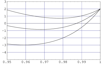
Figure 1: $(\tilde{m}_{\phi 0}^{2}(u)+\tilde{m}_{\overline{\phi}}^{2}(u))/\tilde{m}_{0}^{2}$ vs. $u$. The upper, middle and lower solid curves are for the cases of the parameter $r_{2}$ to be 3.0, 3.5, 4.0, respectively. Both the parameters $r_{0}$ and $r_{1}$ are taken as 3.0.

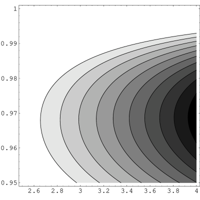
Figure 2: The $u$- and $r_{1}$-dependences of $(\tilde{m}_{\phi 0}^{2}(u)+\tilde{m}_{\overline{\phi}}^{2}(u))/\tilde{m}_{0}^{2}$. The parameter $r_{1}$ varies from 2.5 to 4.0, while the parameters $r_{0}$ and $r_{2}$ are fixed as 3.0 and 3.5, respectively. In the white region $(\tilde{m}_{\phi 0}^{2}(u)+\tilde{m}_{\overline{\phi}}^{2}(u))/\tilde{m}_{0}^{2}$ is positive and in the region from gray to black has a negative value up to $-3.0$.

4 Summary and discussion

In the $SU(6)\times SU(2)_{R}$ string-inspired model with the flavor symmetry ${\bf Z}_{19}\times{\bf Z}_{18}\times\tilde{D}_{4}$, we evolve couplings and masses down from the string scale $M_{S}$ using the RG equations. In the feasible parameter region of a Yukawa coupling and the soft supersymmetry breaking masses, the scalar mass squared of the gauge non-singlet matter field possibly goes negative slightly below the string scale. This implies that the precocious radiative breaking of the gauge symmetry $SU(6)\times SU(2)_{R}$ can occur due to the radiative effect. This symmetry breaking triggers off the subsequent symmetry breaking as

$$SU(6)\times SU(2)_{R}\longrightarrow SU(4)_{PS}\times SU(2)_{L}\times SU(2)_{R}\longrightarrow G_{SM}.$$

Thus the present model is in line with the path from the string scale physics to the low-energy physics.

In the present model, the large Yukawa coupling which plays an important role in the symmetry breaking is identical with the colored Higgs coupling. This is because the superpotential $W_{Y0}$ of Eq.(37) induces the colored Higgs mass term $z_{0}\langle\phi_{0}\rangle g_{0}g_{0}^{c}$ below the scale $\langle\phi_{0}\rangle$. The colored Higgs mass becomes $z_{0}\langle\phi_{0}\rangle={\cal O}(10^{18}{\rm GeV})$. This implies that the proton lifetime is more than $10^{36}$yr. In contrast to the minimal $SU(5)$ SUGRA GUT model, as to which some difficulties have been pointed out concerning the proton lifetime,[20] our result is consistent with the present experimental data[21]. The longevity of the proton is in connection with the precocious gauge symmetry breaking through the common large Yukawa coupling.

References

• [1] K. Inoue, A. Kakuto, H. Komatsu and S. Takeshita, Prog. Theor. Phys. 68, (1982) 927; Prog. Theor. Phys. 71, (1984) 413.
• [2] P. Zoglin, Phys. Lett. 243B, (1990) 215.
• [3] N. Haba, C. Hattori, M. Matsuda and T. Matsuoka, Prog. Theor. Phys. 96, (1996) 1249.
• [4] N. Haba and T. Matsuoka, Prog. Theor. Phys. 99, (1998) 831.
• [5] T. Matsuoka, Prog. Theor. Phys. 100, (1998) 107.
• [6] M. Matsuda and T. Matsuoka, Phys. Lett. B487, (2000) 104.
• [7] M. Matsuda and T. Matsuoka, Phys. Lett. B499, (2001) 287.
• [8] Y. Abe, C. Hattori, M. Ito, M. Matsuda, M. Matsunaga and T. Matsuoka, Prog. Theor. Phys. 106, (2001) 1275.
• [9] Y. Abe, C. Hattori, T. Hayashi, M. Ito, M. Matsuda, M. Matsunaga and T. Matsuoka, hep-ph/0206232.
• [10] N. Haba, C. Hattori, M. Matsuda, T. Matsuoka and D. Mochinaga, Phys. Lett. B337, (1994) 63; Prog. Theor. Phys. 92, (1994) 153.
• [11] J. C. Pati and A. Salam, Phys. Rev. 10, (1974) 275.
• [12] Y. Hosotani, Phys. Lett. B126, (1983) 309; Phys. Lett. B129, (1983) 193.
• [13] P. Candelas, G. T. Horowitz, A. Strominger and E. Witten, Nucl. Phys. B258, (1985) 46.
E. Witten, Nucl. Phys. B258, (1985) 75.
• [14] S. Cecotti, J. P. Derendinger, S. Ferrara, L. Girardello and M. Roncadelli, Phys. Lett. 156B, (1985) 318.
J. D. Breit, B. A. Ovrut and G. C. Segré, Phys. Lett. 158B, (1985) 33.
M. Dine, V. Kaplunovsky, M. Mangano, C. Nappi and N. Seiberg, Nucl. Phys. B259, (1985) 549.
• [15] T. Matsuoka and D. Suematsu, Prog. Theor. Phys. 76, (1986) 886.
N. Haba, C. Hattori, M. Matsuda, T. Matsuoka and D. Mochinaga, Prog. Theor. Phys. 94, (1995) 233.
• [16] C. Froggatt and H. B. Nielsen, Nucl. Phys. B147, (1979) 277.
• [17] S. Coleman and E. Weinberg, Phys. Rev. D7, (1973) 1888.
G. Gamberini, G. Ridolfi and F. Zwirner, Nucl. Phys. B331, (1990) 331.
• [18] V. Kaplunovsky and J. Louis, Phys. Lett. B306, (1993) 269; Nucl. Phys. B444, (1995) 191.
E. Kiritsis and C. Kounnas, Nucl. Phys. B442, (1995) 472.
• [19] N. Falck, Z. Phys. C30 (1986) 247.
• [20] T. Goto and T. Nihei, Phys. Rev. D59, (1999) 115009.
• [21] Super-Kamiokande Collaboration, Phys. Rev. Lett. 83, (1999) 1529.