Renormalization-Mass Scale Dependence in QCD Contributions to Semileptonic $b\rightarrow u$ Decay

Abstract

QCD contributions to the $b\rightarrow u\ell^{-}\overline{\nu}_{\ell}$ decay rate, which are known to two-loop order in the $\overline{MS}$ scheme, exhibit sufficient dependence on the renormalization mass $\mu$ to compromise phenomenological predictions for inclusive semileptonic $B\rightarrow X_{u}$ processes. Such scale dependence is ameliorated by the renormalization-group (RG) extraction and summation of all leading and RG-accessible subleading logarithms occurring subsequent to two-loop order in the perturbative series. This optimal RG-improvement of the known portion of the perturbative series virtually eliminates $\mu$-dependence as a source of theoretical uncertainty in the predicted semileptonic $B\rightarrow X_{u}$ inclusive rate.

The perturbative QCD decay rate $b\rightarrow u\ell^{-}\overline{\nu}_{\ell}$ has been calculated to two-loop (2L) order in the $\overline{MS}$ scheme [1]:

$$\Gamma_{2L}/\kappa = \left[m_{b}(\mu)\right]^{5}\left[1+(4.25360+5L(\mu))x(\mu)\right.$$

$$+ (26.7848+36.9902L(\mu)$$

$$+ \left.17.2917L^{2}(\mu))x^{2}(\mu)\right]$$

$$x(\mu)\equiv\alpha_{s}(\mu)/\pi,\;\;L(\mu)\equiv\log(\mu^{2}/m_{b}^{2}(\mu)),$$

$$\kappa\equiv G_{F}^{2}|V_{ub}|^{2}/192\pi^{3}.$$ (2)

This rate, labelled curve “2L” in Figure 1, exhibits substantial dependence on the $\overline{MS}$ renormalization scale $\mu$. Such dependence, an $O$(15%) decline in rate over the range $2$ GeV $\leq\mu\leq 9$ GeV, is necessarily a source of theoretical uncertainty. Moreover, the 2L rate does not exhibit any extremum in $\mu$ identifiable with a point of minimal sensitivity (PMS) [2], although the one-loop (1L) rate, as given by Eq. (1) without its 2L terms, does have a maximum near $\mu=2.7$ GeV at $\Gamma_{1L}/\kappa\cong 1800$ GeV⁵, as evident from the 1L curve in Fig. 1. Such a maximum, however, is no longer evident in the 2L curve, whose only benchmark value is its closest approach to the 1L curve occurring at $\mu=2.85$ GeV (and $\Gamma_{2L}/\kappa\cong 1890$ GeV⁵). We denote this point, at which the 2L contribution to the rate is a minimum, as the point of fastest apparent convergence (FAC) [3]. We further note from Figure 1 that the 1L and 2L curves exhibit PMS and FAC points at values of $\mu$ much less than the b-quark mass $m_{b}(m_{b})=4.17$ GeV [4] at which all logarithms $L(\mu)$ in Eq. (1) are zero.

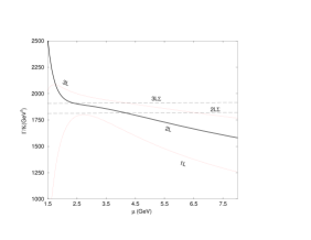
Figure 1: Comparison of one-loop (1L), two-loop (2L), and three-loop (3L) QCD $\overline{MS}$ corrections to the $b\rightarrow u\ell^{-}\overline{\nu}_{\ell}$ decay rate to corresponding rate expressions (2L$\Sigma$ and 3L$\Sigma$) obtained via summation of all leading and subleading higher-order logarithm terms respectively accessible from two-loop and three-loop QCD. All curves are obtained using benchmark values $\alpha_{s}(M_{z})=0.118,\;m_{b}(m_{b})=4.17$ GeV for the evolution of the QCD couplant and running $b$-quark mass via the four-loop $\beta$-function and anomalous mass dimension.

Consequently, there is genuine ambiguity as to which value of $\mu$ is appropriate for theoretical predictions of $|V_{ub}|$ from the inclusive semileptonic $B\rightarrow X_{u}$ decay rate, as well as concomitant theoretical uncertainty in such predictions.

The true decay rate $\Gamma$ is necessarily independent of $\mu$, an unphysical parameter introduced into perturbative QCD as a by-product of the regularization and the removal of infinities. Indeed the statement that the total derivative of $\Gamma$ with respect to $\mu$ must vanish, inclusive of implicit dependence of $\Gamma$ on $\mu$ through the QCD couplant $x(\mu)$ and running mass $m_{b}(\mu)$, leads directly to the renormalization-group equation (RGE)

$$\left[1-2\gamma_{m}(x)\right]\frac{\partial S}{\partial L}+\beta(x)\frac{\partial S}{\partial x}+5\gamma_{m}S=0,$$ (3)

for the perturbative series

$$S\left[x(\mu),L(\mu)\right]=\sum_{n=0}^{\infty}\sum_{k=0}^{n}T_{n,k}x^{n}L^{k}$$ (4)

$$T_{0,0}=1,\;T_{1,0}=4.25360,\;T_{1,1}=5,$$

$$T_{2,0}=26.7848,T_{2,1}=36.9902,T_{2,2}=17.2917$$ (5)

within Eq. (1). If we substitute the series (4) into the RGE (3), we obtain the following set of recursion relations by requiring that the aggregate coefficients of $x_{n}L^{n-1},\;x_{n}L^{n-2}$, and $x_{n}L^{n-3}$ in the RGE (with $\beta(x)=-\sum_{n=0}^{\infty}\beta_{n}x^{n+2}$ and anomalous mass dimension $\gamma_{m}(x)=-\sum_{n=0}^{\infty}\gamma_{n}x^{n+1}$) respectively vanish:

$$nT_{n,n}-\left[\beta_{0}(n-1)+5\gamma_{0}\right]T_{n-1,n-1}=0,\;n\geq 1$$ (6)

$$0=(n-1)T_{n,n-1}+2\gamma_{0}(n-1)T_{n-1,n-1}$$

$$-\beta_{0}(n-1)T_{n-1,n-2}-\beta_{1}(n-2)T_{n-2,n-2}$$

$$-5\gamma_{0}T_{n-1,n-2}-5\gamma_{1}T_{n-2,n-2},\;n\geq 2$$ (7)

$$0 = (n-2)T_{n,n-2}+2\gamma_{0}(n-2)T_{n-1,n-2}$$ (8)

$$+ 2\gamma_{1}(n-2)T_{n-2,n-2}-\beta_{0}(n-1)T_{n-1,n-3}$$

$$- \beta_{1}(n-2)T_{n-2,n-3}-\beta_{2}(n-3)T_{n-3,n-3}$$

$$- 5\gamma_{0}T_{n-1,n-3}-5\gamma_{1}T_{n-2,n-3}$$

$$- 5\gamma_{2}T_{n-3,n-3},\;\;n\geq 3$$

The recursion relation (6) can be utilised to determine any coefficient $T_{n,n}$ in (4), given knowledge of $T_{0,0}(\equiv 1)$. Once all $T_{n,n}$ are known, the recursion relation (7) can be utilised to determine any coefficient $T_{n,n-1}$ from knowledge of $T_{1,0}$, as given by Eq. (5), and with this knowledge, the recursion relation (8) can be employed to determine any coefficient $T_{n,n-2}$ from knowledge of $T_{2,0}$ [Eq.(5)]. Upon rearrangement of the series (4) into the form

$$S[x(\mu),L(\mu)]=\sum_{n=0}^{\infty}x^{n}S_{n}(xL),$$

$$S_{n}(u)=\sum_{k=n}^{\infty}T_{k,k-n}u^{k-n}$$ (9)

we thus see that the leading three coefficients $S_{0}(xL)$, $S_{1}(xL)$, and $S_{2}(xL)$ are fully determined by the recursion relations (6-8) and the values of $T_{0,0}$, $T_{1,0}$, and $T_{2,0}$ already known from the two-loop calculation (1). The detailed mathematical evaluation of these coefficients $S_{n}(xL)$ is presented in ref. [5], and leads to an optimal RG-improvement of the two-loop rate,

$$\Gamma_{2L\Sigma}/\kappa=[m_{b}(\mu)]^{5}[S_{0}+S_{1}x(\mu)+S_{2}x^{2}(\mu)]$$ (10)

$$S_{0}=\left[1-\frac{23}{12}x(\mu)L(\mu)\right]^{-60/23}$$ (11)

$$S_{1} = -\frac{18655}{3174}\left[1-\frac{23}{12}x(\mu)L(\mu)\right]^{-60/23}$$ (12)

$$+ \left\{10.1310+\frac{1020}{529}\log\left[1-\frac{23}{12}x(\mu)L(\mu)\right]\right\}$$

$$\times \left[1-\frac{23}{12}x(\mu)L(\mu)\right]^{-83/23}$$

$$S_{2} = 13.2231\left[1-\frac{23}{12}x(\mu)L(\mu)\right]^{-60/23}$$ (13)

$$- \left\{47.4897+\frac{3171350}{279841}\right.$$

$$\times \left.\log\left[1-\frac{23}{12}x(\mu)L(\mu)\right]\right\}$$

$$\times \left[1-\frac{23}{12}x(\mu)L(\mu)\right]^{-83/23}+\left\{61.0515\right.$$

$$+ 25.5973\log\left[1-\frac{23}{12}x(\mu)L(\mu)\right]$$

$$+ \frac{719610}{279841}\left.\log^{2}\left[1-\frac{23}{12}x(\mu)L(\mu)\right]\right\}$$

$$\times \left[1-\frac{23}{12}x(\mu)L(\mu)\right]^{-106/23}$$

whose dependence on $\mu$ is virtually eliminated. The $2L\Sigma$ curve in Fig. 1, as determined from Eq. (10), is almost flat over the range of $\mu$ indicated: $\Gamma_{2L\Sigma}/\kappa=1816\pm 6$ GeV⁵.

To obtain some control over 2L-order series truncation, we utilise an asymptotic Padé-approximant determination of $T_{3,0}=206$ [6] in conjunction with the RGE (3) to estimate the three-loop rate:

$$\frac{\Gamma^{N^{3}L}}{\mathcal{K}} = \left[m_{b}(\mu)\right]^{5}\left\{1+(4.25360+5L(\mu))x(\mu)\right.$$ (14)

$$+ \left(26.7848+36.9902L(\mu)\right.$$

$$+ \left.17.2917L^{2}(\mu)\right)x^{2}(\mu)$$

$$+ \left(206+249.592L(\mu)+178.755L^{2}(\mu)\right.$$

$$+ \left.\left.50.9144L^{3}(\mu)\right)x^{3}(\mu)\right\}$$

The plot of this 3L rate in Fig. 1 indicates both a PMS maximum and an FAC point (at which the 3L term in Eq. (14) vanishes) at very low values of $\mu\;(\cong 1.8$ GeV $)$, after which the rate falls off with increasing $\mu$ somewhat less steeply than $\Gamma_{2L}/\kappa$. However, given knowledge of $T_{3,0}$, the RGE (3) may be used as above to calculate a recursion relation which determines all coefficients $T_{n,n-3}$:

$$0 = (n-3)\left[T_{n,n-3}+2\gamma_{0}T_{n-1,\;n-3}\right.$$

$$+ \left.2\gamma_{1}T_{n-2,\;n-3}+2\gamma_{2}T_{n-3,\;n-3}\right]$$

$$- \beta_{0}(n-1)T_{n-1,\;n-4}-\beta_{1}(n-2)T_{n-2,\;n-4}$$

$$- \beta_{2}(n-3)T_{n-3,\;n-4}-\beta_{3}(n-4)T_{n-4,\;n-4}$$

$$- 5\gamma_{0}T_{n-1,\;n-4}-5\gamma_{1}T_{n-2,\;n-4}$$

$$- 5\gamma_{2}T_{n-3,\;n-4}-5\gamma_{3}T_{n-4,\;n-4},\;\;\;n\geq 4.$$

This relation determines all coefficients within the Eq. (9) series expression for $S_{3}(xL)$ [5]:

$$S_{3} = -\frac{4.7895}{(1-\frac{23}{12}xL)^{60/23}}$$

$$+ \frac{[60.617+25.496\log(1-\frac{23}{12}xL)]}{(1-\frac{23}{12}xL)^{83/23}}$$

$$+ \left[-198.79-118.29\log(1-\frac{23}{12}xL)\right.$$

$$- \left.15.114\log^{2}(1-\frac{23}{12}xL)\right]/(1-\frac{23}{12}xL)^{106/23}$$

$$+ \left[348.96+189.05\log(1-\frac{23}{12}xL)\right.$$

$$+ 41.697\log^{2}(1-\frac{23}{12}xL)$$

$$+ \left.2.9199\log^{3}(1-\frac{23}{12}xL)\right]/(1-\frac{23}{12}xL)^{129/23}$$

In Fig. 1, the 3L$\Sigma$ curve $[m_{b}(\mu)]^{5}[S_{0}+S_{1}x(\mu)+S_{2}x^{2}(\mu)+S_{3}x^{3}(\mu)]$ is plotted, based upon the estimated value $S_{3}(0)=T_{3,0}=206$, and is seen to be even flatter than the 2L$\Sigma$ curve: $\Gamma_{3L\Sigma}/\kappa=1912\pm 4$ GeV⁵ over the region of $\mu$ displayed. This value is 5% larger than the 2L$\Sigma$ rate, indicative of the truncation error from ignoring higher order terms. Note that this estimate of truncation error is fully decoupled from renormalization scale dependence, which is virtually eliminated from both $2L\Sigma$ and (estimated) 3L$\Sigma$ rates. Curiously, $\Gamma_{2L\Sigma}$, the optimally RG-improved two-loop rate, is quite close to the PMS maximum of the one-loop rate $\Gamma_{1L}$, and that $\Gamma_{3L\Sigma}$, the optimally RG-improved three-loop rate, is quite close to the FAC prediction of the two-loop rate $\Gamma_{2L}$, suggesting that such benchmark points may anticipate higher order calculations.

We are grateful for hospitality from the KEK Theory Group, where this research was initiated, and for support from the Natural Sciences and Engineering Research Council of Canada.

References

[1] T. van Ritbergen, Phys. Lett. B 454 (1999) 353;
T. Seidensticker and M. Steinhauser, Phys. Lett. B 467 (1999) 271.
[2] P. M. Stevenson, Phys. Rev. D 23 (1981) 2916.
[3] G. Grunberg, Phys. Lett. B 95 (1980) 70 and Phys. Rev. D 29 (1984) 2315.
[4] K. G. Chetyrkin and M. Steinhauser, Phys. Rev. Lett. 83 (1981) 4001.
[5]M. R. Ahmady et al., Phys. Rev. D 66 (2002) 014010.
[6]M. R. Ahmady, F. A. Chishtie, V. Elias and T. G. Steele, Phys. Lett. B 479 (2000) 201.