Radiative Neutralino Decay in Supersymmetric Models

Abstract:

The radiative decay $\widetilde{Z}_{2}\rightarrow\widetilde{Z}_{1}\gamma$ proceeds at the one-loop level in the MSSM. It can be the dominant decay mode for the second lightest neutralino $\widetilde{Z}_{2}$ in certain regions of parameter space of supersymmetric models, where either a dynamical and/or kinematic enhancement of the branching fraction occurs. We perform an updated numerical study of this decay mode in both the minimal supergravity model (mSUGRA) and in the more general MSSM framework. In mSUGRA, the largest rates are found in the “focus point” region, where the $\mu$ parameter becomes small, and the lightest neutralinos become higgsino-like; in this case, radiative branching fraction can reach the 1% level. Our MSSM analysis includes a scan over independent positive and negative gaugino masses. We show branching fractions can reach the 10-100% level even for large values of the parameter $\tan\beta$. These regions of parameter space are realized in supergravity models with non-universal gaugino masses. Measurement of the radiative neutralino branching fraction may help pin down underlying parameters of the fundamental supersymmetric model.

1 Introduction

One of the major goals of collider experiments is to verify or disprove the existence of weak scale supersymmetric matter[1]. Given sufficient energy and integrated luminosity, sparticles should be produced at large rates, if indeed they exist. Once produced, sparticles will decay via a cascade into other sparticles until the state containing the lightest SUSY particle (LSP) is reached[2]. If kinematically accessible, tree level two-body decays will comprise the dominant sparticle branching fractions. If two-body modes are suppressed or closed, then tree level three-body decays can dominate. It is also possible for sparticles to decay into two-body final states where the decay is mediated by loop diagrams. Important examples include $\tilde{g}\rightarrow g\widetilde{Z}_{i}$, $\widetilde{Z}_{i}\rightarrow\widetilde{Z}_{j}\gamma$ ($i,j=1-4$ with $i>j$) and $\tilde{t}_{1}\rightarrow c\widetilde{Z}_{1}$ for sparticles, and $h\rightarrow\gamma\gamma$ for the lightest SUSY Higgs scalar.

The radiative decay $\widetilde{Z}_{i}\rightarrow\widetilde{Z}_{j}\gamma$ has been examined previously in a number of papers, since it can give rise to a distinctive energetic, isolated photon plus missing energy signature. The decay proceeds through loops containing intermediate charged scalars and charginos. After several approximate calculations[3], the complete calculation was presented in both the non-linear and linear $R_{\xi}$ gauge by Haber and Wyler[4]. These authors note that the radiative neutralino decay branching fraction may be large in MSSM parameter space regions where $M_{1},\ M_{2},\ |\mu|\ll M_{Z}$ (light neutralino radiative decay), or when $|\mu|,M_{Z}\ll M_{1},\ M_{2}\sim$ TeV (higgsino to higgsino radiative decay).

Detailed numerical studies of the $\widetilde{Z}_{2}\rightarrow\widetilde{Z}_{1}\gamma$ decay rate have been performed by Ambrosanio and Mele[5]. These authors found that the $\widetilde{Z}_{2}\rightarrow\widetilde{Z}_{1}\gamma$ decay rate can in fact be the dominant $\widetilde{Z}_{2}$ decay mode in regions of MSSM model parameter space where tree level two-body $\widetilde{Z}_{2}$ decay modes are not allowed, and the competing $\widetilde{Z}_{2}$ three-body decay modes are dynamically and/or kinematically suppressed.

At low $\tan\beta$, the three-body neutralino decay $\widetilde{Z}_{2}\rightarrow\widetilde{Z}_{1}f\bar{f}$ occurs dominantly via five Feynman diagrams involving virtual sfermion and $Z$ boson exchange. The dynamical suppression of the three-body decay modes occurs when one of $\widetilde{Z}_{2}$ and $\widetilde{Z}_{1}$ is gaugino-like, while the other is higgsino-like. Since the $\widetilde{Z}_{i}f\tilde{f}$ vertex contains the gaugino component of the neutralinos, the decay via a virtual sfermion $\tilde{f}^{*}$ is suppressed if one (or both) of $\widetilde{Z}_{2}$ or $\widetilde{Z}_{1}$ is higgsino-like. In addition, the $Z\widetilde{Z}_{2}\widetilde{Z}_{1}$ coupling contains the higgsino components of the neutralinos so that if one of $\widetilde{Z}_{1}$ and/or $\widetilde{Z}_{2}$ is gaugino-like, then decay via the $Z^{*}$ diagram is suppressed. The region of MSSM parameter space where dynamical suppression of three-body decay modes occurs is when the gaugino masses $M_{1}\sim M_{2}$, $\tan\beta\sim 1$ and $\mu<0$ with $|\mu|$ being sufficiently small. In light of recent limits from LEP2 that $m_{\widetilde{W}_{1}}>103.5$ GeV and $m_{h}>114.1$ GeV (for a SM-like $h$ boson), the region of dynamical suppression is largely excluded, since $m_{h}$ is quite light at very low values of $\tan\beta$.

In addition, there can exist a region of reduced dynamical suppression. In this case, three-body decays via $Z^{*}$ can be suppressed if one (or both) of the neutralinos is gaugino-like (thus suppressing $\widetilde{Z}_{2}$ decay via $Z^{*}$), while the sfermions are quite heavy (thus suppressing decay through $\tilde{f}^{*}$). This interesting case occurs naturally as we shall see in the “focus-point” scenario[6] of the minimal supergravity (mSUGRA or CMSSM) model[7].

Finally, there can exist regions of kinematical suppression of three-body $\widetilde{Z}_{2}$ decays. In this case, $m_{\widetilde{Z}_{2}}\sim m_{\widetilde{Z}_{1}}$ so that $\widetilde{Z}_{2}\rightarrow\widetilde{Z}_{1}f\bar{f}$ is suppressed kinematically by a factor $\epsilon^{5}$, where $\epsilon=(1-m_{\widetilde{Z}_{1}}/m_{\widetilde{Z}_{2}})$. The radiative decay $\widetilde{Z}_{2}\rightarrow\widetilde{Z}_{1}\gamma$ is suppressed by $\epsilon^{3}$, so that as the $m_{\widetilde{Z}_{2}}-m_{\widetilde{Z}_{1}}$ mass gap approaches zero, the radiative decay increasingly dominates. The kinematic suppression region occurs when $\tan\beta\sim 1$ or when $M_{1}\sim M_{2}$. In the region of parameter space where kinematical suppression occurs, however, the small mass gap between neutralinos also means that the final state photon energy will be small, unless enhanced by a Lorentz boost if $\widetilde{Z}_{2}$ is produced either directly or via cascade decay with a high velocity.

The radiative neutralino decays have received some recent attention by Kane et al.[8] in attempts to explain an $ee\gamma\gamma$ event seen by the CDF experiment in run 1 of the Fermilab Tevatron[9]. These “higgsino-world” scenarios seem to need $\tan\beta\sim 1$, $\mu<0$ and a light top squark. These scenarios seem largely excluded now by LEP2 limits on the masses of the Higgs bosons, which require $\tan\beta>2-3$.

In this paper, we re-examine the radiative neutralino decay branching fraction as a function of supersymmetric model parameter space. Our calculations include a number of improvements over previous analyses.

1. We implement the complete $\widetilde{Z}_{2}\rightarrow\widetilde{Z}_{1}\gamma$ decay calculation into the event generator ISAJET v7.64[10]. Our calculation includes full third generation mixing effects amongst the squarks and sleptons.

2. Our treatment of neutralino three-body decays includes the effect of all third generation Yukawa couplings and sfermion mixings in the decay calculations[11]. These are especially important at large values of the parameter $\tan\beta$, where the Yukawa couplings $f_{b}$ and $f_{\tau}$ can become large. In addition, along with the five $\widetilde{Z}_{2}\rightarrow\widetilde{Z}_{1}f\bar{f}$ decay diagrams proceeding via sfermion and $Z$ boson exchange, we include decays through $h$, $H$ and $A$ bosons. These diagrams can be important, especially at large $\tan\beta$[11, 12, 13].

3. We include the latest constraints from LEP2. As noted before, these constraints eliminate many of the regions of parameter space where $\widetilde{Z}_{2}\rightarrow\widetilde{Z}_{1}\gamma$ can be large, especially around $\tan\beta\sim 1$.

4. We present results for the paradigm mSUGRA model. We also present a scan of MSSM parameter space which includes negative as well as positive gaugino masses. We find the radiative decay branching fraction can be large in a particular SUGRA model with non-univeral gaugino masses.

5. Finally, in our numerical scans, we take note of parameter space regions where the radiative neutralino branching fraction is not dominant, but may be nonetheless observable. For instance, at the CERN LHC, many millions of sparticle production events may be recorded each year, provided sparticles are light enough. In this case, branching fractions of a few per cent or even less may be interesting, and allow one to measure the neutralino radiative decay branching fraction. Since the $\widetilde{Z}_{2}\rightarrow\widetilde{Z}_{1}\gamma$ branching fraction is very sensitive to parameter space, its measurement may help determine or constrain some of the fundamental SUSY model parameters.

The rest of this paper is organized as follows. In Sec. 2, we examine the radiative neutralino branching fraction in the mSUGRA model. We find it can reach levels approaching 1%, especially in the well-motivated focus-point region. In Sec. 3, we examine the radiative decay branching fraction in the MSSM. In this case, we find regions of parameter space where the branching fraction can approach 50-100%, even for large values of $\tan\beta$. These regions occur dominantly where $M_{1}\sim M_{2}$ or when $M_{1}\sim-M_{2}$. We note in Sec. 4 that the latter MSSM regions of enhancement naturally occur in a particular SUGRA model with non-universal gaugino masses. We map out the interesting regions of parameter space where the radiative decay branching fraction can be large. Finally, in an appendix, we present our formulae for radiative neutralino production, cast in a form consistent with the ISAJET event generator program.

2 $\widetilde{Z}_{2}\rightarrow\widetilde{Z}_{1}\gamma$ branching fraction in mSUGRA model

Our first goal is to examine the radiative neutralino branching fraction in the paradigm mSUGRA (or CMSSM) model. Most analyses of supersymmetric phenomena take place within this model, so it is convenient to know the rates for radiative neutralino decay in relation to other expected phenomena. In the mSUGRA model, the MSSM is assumed to be valid between the grand unified scale ($M_{GUT}\simeq 2\times 10^{16}$ GeV) and the weak scale ($\sim 1$ TeV). At $M_{GUT}$, it is assumed all scalar masses are unified to the parameter $m_{0}$, while all gaugino masses unify to $m_{1/2}$. In addition, trilinear soft SUSY breaking masses unify to $A_{0}$. The gauge and Yukawa couplings and soft SUSY breaking parameters evolve from $M_{GUT}$ to $M_{weak}$ according to the well-known MSSM renormalization group equations (RGEs). At $M_{weak}$ it is assumed electroweak symmetry is broken radiatively, which fixes the magnitude of the superpotential $\mu$ parameter, and allows one to effectively trade the bilinear soft breaking parameter $B$ for the ratio of Higgs vevs $\tan\beta$. Thus the parameter space is characterized by

$$m_{0},\ m_{1/2},\ A_{0},\ \tan\beta\ \ {\rm and}\ \ sign(\mu),$$ (1)

where we take the top quark pole mass $m_{t}=175$ GeV. In our mSUGRA model calculations, we utilize the iterative RGE solution embedded within the program ISAJET v7.64[10]. This version also includes our radiative neutralino decay calculation.

In Fig. 1, we show the $m_{0}\ vs.\ m_{1/2}$ plane for $\tan\beta=10$, $A_{0}=0$ and $\mu>0$. The red-shaded regions are excluded either by the presence of a stau LSP (upper left) or a lack of REWSB (lower and right). The pink shaded region is excluded by LEP2 searches for charginos and a light Higgs scalar. The upper and left regions indicate where $\widetilde{Z}_{2}$ two-body decays occur: either to $\tilde{\ell}_{1}\ell$ ($\ell$ denotes any of the charged or neutral leptons) on the left, or to $\widetilde{Z}_{1}Z$ or $\widetilde{Z}_{1}h$ in the upper plane. The remaining regions allowed by LEP2 have dominant three-body $\widetilde{Z}_{2}$ decays. The green shaded region has $0.001<BF(\widetilde{Z}_{2}\rightarrow\widetilde{Z}_{1}\gamma)<0.005$ while the yellow has $0.005<BF(\widetilde{Z}_{2}\rightarrow\widetilde{Z}_{1}\gamma)<0.01$. In these regions, where $m_{1/2}\stackrel{{\scriptstyle<}}{{\sim}}250$ GeV, we also have $m_{\tilde{g}}\stackrel{{\scriptstyle<}}{{\sim}}650$ GeV. Then $\tilde{g}\tilde{g}$ cross sections exceed $\sim 2000$ fb at the CERN LHC, leading to at least 20,000 SUSY events per 10 fb^-1 of integrated luminosity. After suitable cuts are made on number of jets, jet $E_{T}$ and $\not\!\!{E_{T}}$, a nearly pure sample of SUSY events will remain[14]. These SUSY candidates can then be scrutinized for the presence of hard, isolated photons, and may allow a determination at some level of the neutralino radiative decay branching fraction.

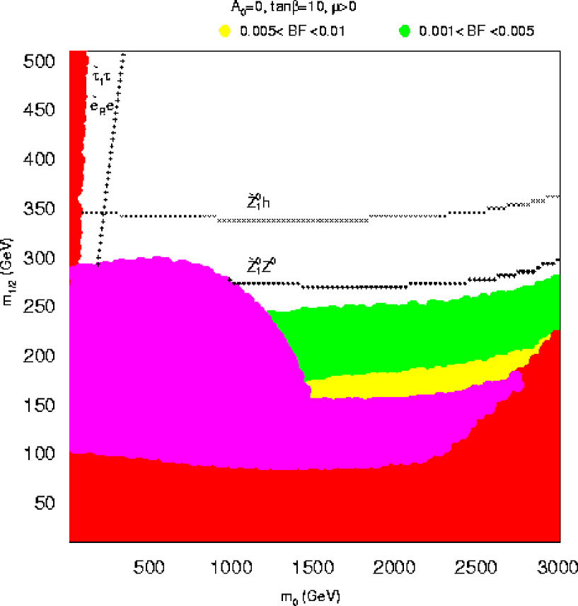
Figure 1: Regions of mSUGRA model parameter space with significant $\widetilde{Z}_{2}\rightarrow\widetilde{Z}_{1}\gamma$ branching fraction, in the $m_{0}\ vs.\ m_{1/2}$ plane for $\tan\beta=10$, $A_{0}=0$ and $\mu>0$. The red shaded regions are theoretically excluded while pink regions are excluded by sparticle searches at LEP2. The green region has $0.001<BF(\widetilde{Z}_{2}\rightarrow\widetilde{Z}_{1}\gamma)<0.005$, while the yellow region has $0.005<BF(\widetilde{Z}_{2}\rightarrow\widetilde{Z}_{1}\gamma)<0.01$.

We note that the regions of mSUGRA parameter space with the largest $\widetilde{Z}_{2}\rightarrow\widetilde{Z}_{1}\gamma$ branching fraction occur at rather large $m_{0}$ and low $m_{1/2}$ values. The very largest allowed $m_{0}$ areas correspond to the focus-point region of Feng, Matchev and Moroi[6], where fine-tuning may be low, but squark and slepton masses are at the multi-TeV level. These heavy sfermion masses may be sufficient to suppress many flavor-changing or $CP$ violating processes that could arise due to the presence of off-diagonal flavor changing soft SUSY masses, or imaginary components of soft SUSY breaking terms.

We also show the regions of $\widetilde{Z}_{2}\rightarrow\widetilde{Z}_{1}\gamma$ branching fraction for large $\tan\beta=45$ in Fig. 2. Again, we see a significant part of the three-body $\widetilde{Z}_{2}$ decay region inhabited with possibly measurable branching fractions for radiative neutralino decay. The region with the largest branching fraction is adjacent to the right-side region forbidden by lack of REWSB. In that region, the $\mu$ parameter is becoming small, and the light neutralinos are becoming increasingly higgsino-like. In addition, sfermion masses are heavy, so we are in a region of reduced dynamical suppression of three-body decay modes, also with some kinematic suppression.

In both the low and the high $\tan\beta$ cases, it is important to note that the $\widetilde{Z}_{2}\rightarrow\widetilde{Z}_{1}\gamma$ branching fraction reaches no greater than 1%, so is never dominant. However, regions do occur where the radiative decay should be detectable, and the branching fraction should be measureable. Detailed simulations including detector effects for identifying isolated photons will be necessary to ascertain the precision with which such measurements can be made.

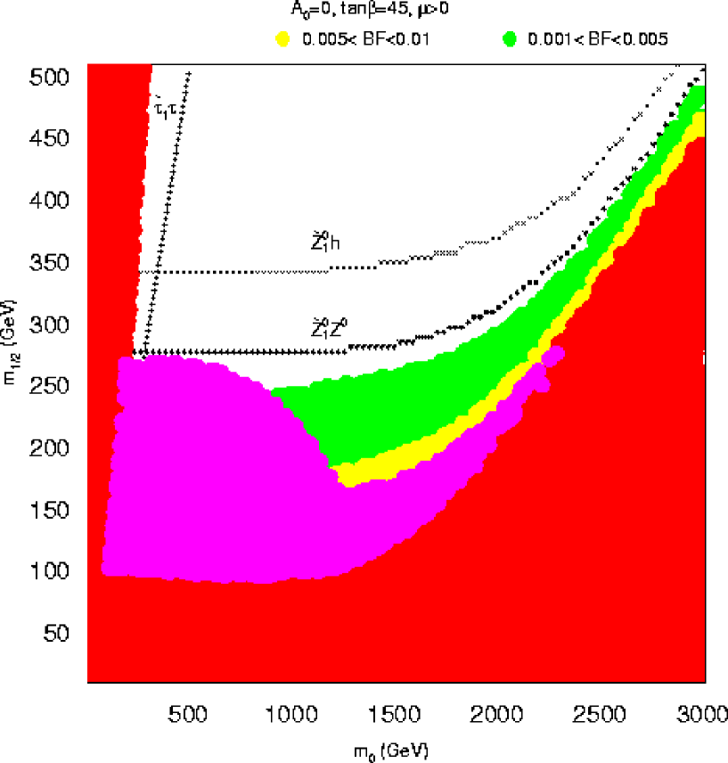
Figure 2: Same as Fig. 1, except $\tan\beta=45$.

3 $\widetilde{Z}_{2}\rightarrow\widetilde{Z}_{1}\gamma$ branching fraction in the MSSM

It is apparent from the numerical studies of Ambrosanio and Mele[5] that the greater freedom of parameter choices in the unconstrained MSSM can allow for regions of parameter space with larger $\widetilde{Z}_{2}\rightarrow\widetilde{Z}_{1}\gamma$ branching fractions than in the mSUGRA model. In this section, we present a scan over unconstrained MSSM parameters. To make the analysis tractable, we do assume all MSSM soft SUSY breaking parameters and Yukawa couplings to be purely real, and we take all sfermion masses to be degenerate, with no intergenerational mixing. For simplicity, we take $A_{t}=A_{b}=A_{\tau}$, and fix $m_{\tilde{g}}=1500$ GeV. Our scan of MSSM parameter space is then over the following region:

$$-1500\ {\rm GeV}< M_{1} <1500\ {\rm GeV},$$

$$0< M_{2} <1500\ {\rm GeV},$$

$$-1500\ {\rm GeV}< \mu <1500\ {\rm GeV},$$

$$-2000\ {\rm GeV}< A_{t} <2000\ {\rm GeV},$$

$$150\ {\rm GeV}< m_{A} <1500\ {\rm GeV},$$

$$2< \tan\beta <50,$$

$$100\ {\rm GeV}< m_{\tilde{f}} <1500\ {\rm GeV},$$

where we have the freedom to choose one of the gaugino masses, in this case $M_{2}$, to be real and positive. We require $m_{\widetilde{W}_{1}}>103.5$ GeV and $m_{h}>114.1$ GeV, according to LEP2. The latter Higgs mass requirement is overly harsh in that the limit on the lightest SUSY Higgs boson is somewhat lower, but this doesn’t alter our conclusions. We also require a mass gap $m_{\widetilde{Z}_{2}}-m_{\widetilde{Z}_{1}}>5$ GeV, so that the photon that appears in scattering events from any of these models has a detectable energy.

Our results are presented in Figs. 3 and 4, as plots of branching fraction ($BF$) versus model parameter. Fig. 3a and 3b show the branching fractions versus the gaugino masses $M_{1}$ and $M_{2}$. We see immediately that in fact there do exist models with substantial radiative decay branching fractions in the range 10%-100%. For both gaugino masses, these large branching fraction models populate the region with $|M_{1}|,\ M_{2}<1000$ GeV, with the distribution of points being somewhat asymmetric for $M_{1}$ being positive or negative. If $M_{1}$ becomes large negative or $M_{2}$ becomes large, the branching fractions can remain large, but the mass gap $m_{\widetilde{Z}_{2}}-m_{\widetilde{Z}_{1}}$ decreases below 5 GeV. However, for large positive $M_{1}$ the mass gap stays large, but in this case we do not get large branching fractions because either two-body decay modes of $\widetilde{Z}_{2}$ turn on, or else $\widetilde{Z}_{2}\rightarrow\widetilde{W}_{1}f\bar{f}^{\prime}$ becomes large, thus supressing the radiative decay branching fraction. The models with $|M_{1}|,\ M_{2}$ near zero are usually excluded by constraints from LEP on $Z\rightarrow\widetilde{Z}_{i}\widetilde{Z}_{j}$ decay or from LEP2 on the chargino mass.

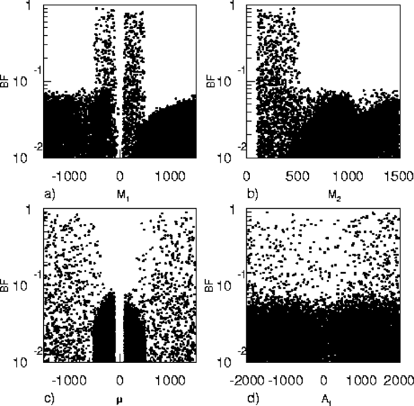
Figure 3: Plot of $BF(\widetilde{Z}_{2}\rightarrow\widetilde{Z}_{1}\gamma)$ versus the parameter a) $M_{1}$, b) $M_{2}$, c) $\mu$ and d) $A_{t}$ in the MSSM model.

Fig. 3c shows the $BF$ versus the $\mu$ parameter. Again, small values of $|\mu|$ are excluded by LEP and LEP2 constraints. However, we see that really large radiative decay branching fractions only occur for very large values of $|\mu|\stackrel{{\scriptstyle>}}{{\sim}}300-400$ GeV. The suppresion of lower values of $|\mu|$ comes from the mass gap requirement. Fig. 3d shows the branching fraction versus the parameter $A_{t}$. Here, large values of branching fraction are possible for all values of $A_{t}$, although the very largest seem to favor large values of $|A_{t}|$.

In Fig. 4 we show the $BF$ versus the parameters $m_{A}$, $\tan\beta$ and $m_{\tilde{f}}$ in frames a, b and c. We see that large branching fractions are possible for all values of pseudoscalar mass $m_{A}$, and for all values of $\tan\beta$. Large values of BF have some preference for $m_{\tilde{f}}\stackrel{{\scriptstyle>}}{{\sim}}300-400$ GeV, so that two-body decays $\widetilde{Z}_{2}\rightarrow f\tilde{f}$ are closed, and three-body decays $\widetilde{Z}_{2}\rightarrow\widetilde{Z}_{1}f\bar{f}$ through an intermediate $\tilde{f}$ have some suppression.

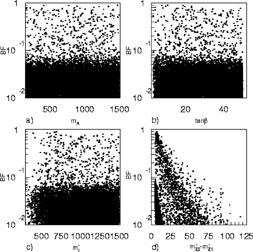
Figure 4: Plot of $BF(\widetilde{Z}_{2}\rightarrow\widetilde{Z}_{1}\gamma)$ versus the parameter a) $m_{A}$, b) $\tan\beta$, c) $m_{\tilde{f}}$ and d) $m_{\widetilde{Z}_{2}}-m_{\widetilde{Z}_{1}}$ in the MSSM model.

In the last frame, Fig. 4d, we show the branching fraction not against an input parameter, but against the neutralino mass gap, $m_{\widetilde{Z}_{2}}-m_{\widetilde{Z}_{1}}$. Here it is clear that the largest values of $BF$ prefer the smallest mass gaps, where there exists at least some amount of kinematical suppression of three-body $\widetilde{Z}_{2}$ decays. The large branching fractions have a cut-off around 90-100 GeV, where $\widetilde{Z}_{2}\rightarrow\widetilde{Z}_{1}Z$ decays become possible.

To gain more understanding of the parameter space where radiative decays are large, we plot in Fig. 5 only models with $BF>10\%$ (black dots) or $>1\%$ (red dots), in correlated parameter planes. Again, we require $m_{\widetilde{Z}_{2}}-m_{\widetilde{Z}_{1}}>5$ GeV, and all LEP and LEP2 constraints to be satisfied. From Fig. 5a in the $M_{1}\ vs.\ M_{2}$ plane, we see that models with the largest $BF$ require $|M_{1}|\sim M_{2}$, a feature noted by Ambrosanio and Mele in their analysis[5]. The region with $M_{1}\sim M_{2}$ turns out to be quite narrow, while the region with $M_{1}\sim-M_{2}$ has slightly more breadth to it. This latter point is even more apparent when we relax to the condition $BF>1\%$.

In Fig. 5b and 5c, we show models in the $M_{1}\ vs.\ \mu$ and $M_{2}\ vs.\ \mu$ planes. For models with $BF>10\%$, evidently $|M_{1}|<|\mu|$ and also $M_{2}<|\mu|$. If we relax to models with $BF>1\%$, then these requirements no longer hold. In frame 5d, we show models in the $M_{2}/M_{1}\ vs.\ \mu$ plane. Models with $BF>10\%$ clearly favor $M_{2}/M_{1}\sim 1$, with either sign of $\mu$ being equally preferable. If we allow models with $BF>1\%$, then the $M_{1}\sim\pm M_{2}$ restriction can be relaxed, and rather large ratios of $M_{2}/M_{1}$ are allowed, especially if $|\mu|$ is small.

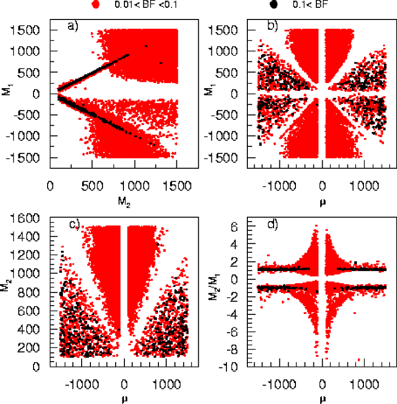
Figure 5: Plot of MSSM model points with $BF(\widetilde{Z}_{2}\rightarrow\widetilde{Z}_{1}\gamma)>0.1$ and $m_{\widetilde{Z}_{2}}-m_{\widetilde{Z}_{1}}>5$ GeV in a) $M_{1}\ vs.\ M_{2}$ space, b) $M_{1}\ vs.\ \mu$ space, c) $M_{2}\ vs.\ \mu$ space and d) $M_{2}/M_{1}\ vs.\ \mu$ space.

An important element of our analysis is the size of the $\widetilde{Z}_{2}-\widetilde{Z}_{1}$ mass gap, so there is sufficient photon energy for observations. In Fig. 6, we show the mass gap $m_{\widetilde{Z}_{2}}-m_{\widetilde{Z}_{1}}$ versus the parameters $\mu$, $M_{1}$, $M_{2}$ and $\tan\beta$ in frames a-d, respectively. From Fig. 6a, we see that models with $BF>10\%$ prefer large absolute values of the $\mu$ parameter, but for these models the mass gap is bounded typically by 40-60 GeV. By relaxing to models with $BF>1\%$, we pick up models with mass gaps ranging to 100 GeV. However, for models with small values of $\mu$, where higgsino$\rightarrow$ higgsino transitions are possible, the mass gap is very small ($\stackrel{{\scriptstyle<}}{{\sim}}20$ GeV), and these cases will be more difficult to observe. Figs. 6b and 6c show that the mass gap for models with $BF>10\%$ is typically less than 30-40 GeV for $|M_{1}|,\ M_{2}$ ranging up to 1000 GeV. The models with $BF>1\%$ and $|M_{1}|,\ M_{2}>1000$ GeV typically have a small mass gap, less than 10-15 GeV. Finally, in Fig. 6d, the mass gap versus $\tan\beta$ shows no major correlations, and significant mass gaps can be achieved for any $\tan\beta$ values.

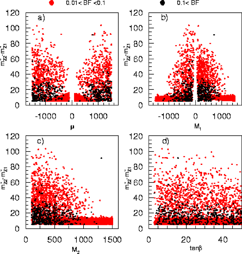
Figure 6: Plot of the mass gap $m_{\widetilde{Z}_{2}}-m_{\widetilde{Z}_{1}}$ versus a) $\mu$, b) $M_{1}$ and c) $M_{2}$ for MSSM model points with $BF(\widetilde{Z}_{2}\rightarrow\widetilde{Z}_{1}\gamma)>0.1$ and $m_{\widetilde{Z}_{2}}-m_{\widetilde{Z}_{1}}>5$ GeV. In d), we plot the mass gap $m_{\widetilde{Z}_{2}}-m_{\widetilde{Z}_{1}}$ versus the parameter $\tan\beta$ in the MSSM.

To conclude this section, we summarize our findings by noting that the largest neutralino radiative decay branching fractions are found in regions of parameter space with

$$|M_{1}|,\ M_{2}\sim 100-1000\ {\rm GeV},$$

$$|\mu|>|M_{1}|,\ M_{2}\ \ {\rm and}$$

$$|M_{1}|\sim M_{2}.$$

4 $\widetilde{Z}_{2}\rightarrow\widetilde{Z}_{1}\gamma$ branching fraction in a SUGRA model with non-universal gaugino masses

So far, our findings are that in the mSUGRA model the radiative decay $BF$ never exceeds 1%, and is largest in regions with large $m_{0}$ such as the focus point region. For the MSSM case, we found distinct regions of parameter space where the radiative branching fraction can range up to 10%-100%, although these conditions are never realized in the mSUGRA model. In this section, we note that there do exist models where the above MSSM parameter space restrictions are realized, namely in SUGRA models with non-universal gaugino masses.

Since supergravity is not a renormalizable theory, in general we may expect a non-trivial gauge kinetic function. Expanding the gauge kinetic function as

$$f_{AB}=\delta_{AB}+\hat{h}_{AB}/M_{P}+\ldots,$$ (2)

where the fields $\hat{h}_{AB}$ transform as left handed chiral superfields under supersymmetry transformations, and as the symmetric product of two adjoints under gauge symmetries, we parametrize the lowest order contribution to gaugino masses by,

$${\cal{L}}\supset-{1\over 4}\int d^{2}\theta_{L}\frac{\hat{h}_{AB}}{M_{P}}\overline{\hat{W}_{A}^{c}}\hat{W}_{B}\supset\frac{\langle F_{h}\rangle_{AB}}{M_{P}}\lambda_{A}\lambda_{B}+\ldots$$ (3)

where the $\hat{W}_{A}$ are curl superfields, the $\lambda_{A}$ are the gaugino fields, and $F_{hAB}$ are the auxillary field components of the $\hat{h}_{AB}$ that acquire a SUSY breaking $vev$.

If the fields $F_{h}$ which break supersymmetry are gauge singlets, universal gaugino masses result. However, in principle, the chiral superfield which communicates supersymmetry breaking to the gaugino fields can lie in any representation in the symmetric product of two adjoints, and so can lead to gaugino mass terms that (spontaneously) break the underlying gauge symmetry.

In the context of $SU(5)$ grand unification, $F_{h}$ belongs to an $SU(5)$ irreducible representation which appears in the symmetric product of two adjoints:

$$({\bf 24}{\bf\times}{\bf 24})_{\rm symmetric}={\bf 1}\oplus{\bf 24}\oplus{\bf 75}\oplus{\bf 200}\,,$$ (4)

where only $\bf 1$ yields universal masses. The relations amongst the various $GUT$ scale gaugino masses have been worked out by Anderson[15]. The relative $GUT$ scale $SU(3)$, $SU(2)$ and $U(1)$ gaugino masses $M_{3}$, $M_{2}$ and $M_{1}$ are listed in Table 1 along with the approximate masses after RGE evolution to $Q\sim M_{Z}$. These scenarios represent the predictive subset of the more general (and less predictive) case of an arbitrary superposition of these representations. The model parameters may be chosen to be,

$$m_{0},\ M_{3}^{0},\ A_{0},\ \tan\beta\ {\rm and}\ sign(\mu),$$ (5)

where $M_{i}^{0}$ is the $SU(i)$ gaugino mass at scale $Q=M_{GUT}$. $M_{2}^{0}$ and $M_{1}^{0}$ can then be calculated in terms of $M_{3}^{0}$ according to Table 1, and the weak scale SUSY particle spectrum can again be calculated using ISAJET v7.64.

	$M_{GUT}$			$M_{Z}$
$F_{h}$	$M_{3}$	$M_{2}$	$M_{1}$	$M_{3}$	$M_{2}$	$M_{1}$
${\bf 1}$	$1$	$\;\;1$	$\;\;1$	$\sim\;6$	$\sim\;\;2$	$\sim\;\;1$
${\bf 24}$	$2$	$-3$	$-1$	$\sim 12$	$\sim-6$	$\sim-1$
${\bf 75}$	$1$	$\;\;3$	$-5$	$\sim\;6$	$\sim\;\;6$	$\sim-5$
${\bf 200}$	$1$	$\;\;2$	$\;10$	$\sim\;6$	$\sim\;\;4$	$\sim\;10$

Table 1: Relative gaugino masses at $M_{GUT}$ and $M_{Z}$ in the four possible $F_{h}$ irreducible representations.

We note that the 75 model leads to weak scale gaugino masses in the ratio $M_{2}:M_{1}\sim 6:-5$, which is approaching the conditions required in Sec. 3 for models with large radiative branching fractions. We adopt the GUT scale gaugino mass boundary conditions of the 75 model, and explore the model parameter space for large radiative decay branching fractions.

Our first results are shown in Fig. 7 in the $M_{3}^{0}\ vs.\ m_{0}$ plane, for $\tan\beta=5$, $A_{0}=0$ and $\mu>0$. Again, the red shaded regions are excluded theoretically, while the pink regions are excluded by constraints from LEP2. The region with mass gap $m_{\widetilde{Z}_{2}}-m_{\widetilde{Z}_{1}}>5$ GeV is indicated between the dotted contours. The substantial green region has branching fractions $BF:\ 1\%-10\%$, while the yellow region has branching fractions in the range $BF:\ 10\%-50\%$. Almost all the large branching fraction region has mass gap $m_{\widetilde{Z}_{2}}-m_{\widetilde{Z}_{1}}<5$ GeV. The value of $|\mu|$ in the yellow region is generally much smaller than $|M_{1}|$ and $M_{2}$, so that $\widetilde{Z}_{2}\rightarrow\widetilde{Z}_{1}\gamma$ consists of a higgsino $\rightarrow$ higgsino transition, with a rather small mass gap between $\widetilde{Z}_{2}$ and $\widetilde{Z}_{1}$; there is significant kinematic suppression of three-body decay rates. In the lower right unshaded regions, the value of $\mu$ is comparable or larger than $|M_{1}|$ and $M_{2}$, and the $\widetilde{Z}_{2}$-$\widetilde{Z}_{1}$ mass gap is usually larger, so three-body decay rates increase, suppressing the radiative decay branching fraction. An exception occurs near $m_{0}\sim 3000$ GeV and $M_{3}^{0}\sim 300$ GeV where the light neutralinos are transitioning between higgsino-like and gaugino-like. In this area, the mass gap drops to very small values of order 1 GeV, and the radiative decay is momentarily enhanced.

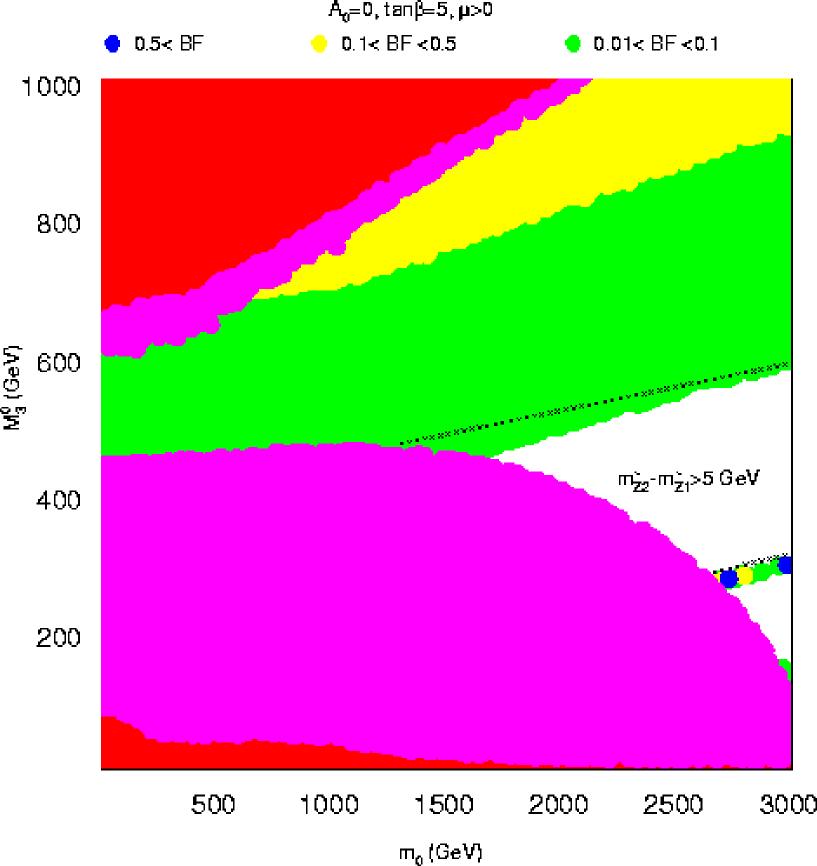
Figure 7: Regions of the 75 SUGRA model parameter space with significant $\widetilde{Z}_{2}\rightarrow\widetilde{Z}_{1}\gamma$ branching fraction, in the $m_{0}\ vs.\ m_{1/2}$ plane for $\tan\beta=5$, $A_{0}=0$ and $\mu>0$. The red shaded regions are theoretically excluded while pink regions are excluded by sparticle searches at LEP2. The green region has $0.01<BF(\widetilde{Z}_{2}\rightarrow\widetilde{Z}_{1}\gamma)<0.1$, while the yellow region has $0.1<BF(\widetilde{Z}_{2}\rightarrow\widetilde{Z}_{1}\gamma)<0.5$.

In Fig. 8, we show again the 75 model, but this time with $\tan\beta=10$. As $\tan\beta$ is increased beyond 5, the allowed parameter space rapidly decreases. In this case, only a small region in the center of the plot gives a viable SUSY spectrum satsifying all constraints. In this case, the yellow region represents $1\%<BF<5\%$ (lower values than in Fig. 7). The larger $\tan\beta$ value allows for a larger mass gap between $\widetilde{Z}_{2}$ and $\widetilde{Z}_{1}$ for small $\mu$ values compared to Fig. 7 ($m_{\widetilde{Z}_{2}}-m_{\widetilde{Z}_{1}}>5$ GeV throughout the $\tan\beta=10$ plane). Consequently, three-body decays suffer less kinematical suppression, and the radiative branching fraction is lower.

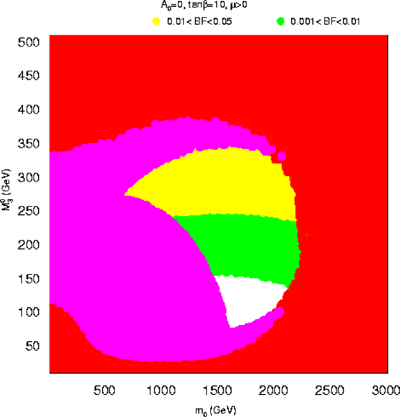
Figure 8: Same as Fig. 6, except $\tan\beta=10$, and now the green region has $0.001<BF(\widetilde{Z}_{2}\rightarrow\widetilde{Z}_{1}\gamma)<0.01$, while the yellow region has $0.01<BF(\widetilde{Z}_{2}\rightarrow\widetilde{Z}_{1}\gamma)<0.05$.

We have also examined briefly two cases of “more minimal” supersymmetric models[16]. In these models, also known as inverted mass hierarchy (IMH) models, there can exist non-universal scalar masses, leading to multi-TeV first and second generation scalars (to suppress flavor and CP violating SUSY processes), while third generation scalars remain in the sub-TeV regime (as required by naturalness constraints). The two models examined were the radiative inverted hierarchy model (RIMH)[17] and the GUT scale IMH model (GSIMH)[18]. In both these models, usually two-body $\widetilde{Z}_{2}$ decays are allowed. In the RIMH model, for some parameter regions the $\mu$ parameter can become very small. In that case, results are similar to the SUGRA model focus point region already presented with branching fractions near the $\sim 1\%$ level.

5 Conclusions

We have re-calculated the decay rate for radiative neutralino decay within the MSSM. We have also made detailed scans of parameter space in the mSUGRA model, the MSSM and a SUGRA model with non-universal gaugino masses. In the mSUGRA model, radiative neutralino branching fractions for $\widetilde{Z}_{2}$ can reach up to 1%. While this rate comprises only a small fraction of the $\widetilde{Z}_{2}$ decay modes, it may be sufficiently large to be measureable at collider experiments at the CERN LHC, where many $\tilde{g}$ and $\tilde{q}$ events can be produced, and $\widetilde{Z}_{2}$ will occur in cascade decays. The rate is largest in the focus point region of parameter space. If the branching fraction is observed, then it may aid in the determination of underlying model parameters.

In the MSSM, the $\widetilde{Z}_{2}\rightarrow\widetilde{Z}_{1}\gamma$ decay rate can reach nearly 100%. In this case, the gaugino masses $|M_{1}|,\ M_{2}\stackrel{{\scriptstyle<}}{{\sim}}1000$ GeV, with $|M_{1}|,\ M_{2}<|\mu|$ and $|M_{1}|\sim M_{2}$. The branching fraction can be large for all values of $\tan\beta$.

The conditions on parameters of the MSSM for a large radiative neutralino branching fraction turn out to be realized in a SUGRA model with non-universal gaugino masses, where the hidden sector field $\hat{h}_{AB}$ transforms as a 75 dimensional symmetric product of two adjoints of $SU(5)$. At low $\tan\beta\sim 5$, in this case the branching fraction can reach up to 50%, although the mass gap $m_{\widetilde{Z}_{2}}-m_{\widetilde{Z}_{1}}$ tends to be rather small - of order a few GeV. For higher $\tan\beta$, the parameter space in the 75 model rapidly diminishes. However, scans made for the $\tan\beta=10$ case show the radiative branching fraction reaching up to $\sim 5\%$.

Our final conclusion is that once a significant sample of SUSY particle candidate events is discovered at collider experiments, then that sample should be scrutinized for the presence of additional isolated photons, beyond the level expected from bremsstrahlung, misidentified jets, etc. If the events contain in addition isolated photons, then it may be possible to test whether they come from radiative neutralino decay, and to in fact measure that particular branching fraction. If the $\widetilde{Z}_{2}\rightarrow\widetilde{Z}_{1}\gamma$ branching fraction is in fact measured, then its value should aid in the attempt to extract the values of underlying model parameters.

Appendix

In this appendix, we present our formulae for the radiative neutralino decay rate. The complete radiative decay width of $\tilde{Z}_{j}$ was calculated by Haber and Wyler[4]. We organize our calculation in a similar fashion to theirs, working in the non-linear $R_{\xi}$ gauge. We use the Lagrangian conventions of Tata[1], which is useful for inclusion into ISAJET. The relevant Feynman diagrams labelled a-p are presented in Ref. [4], and will not be repeated here. We have checked that our formula reproduces analytically that of Haber and Wyler after converting conventions.

In addition, we have compared our numerical results for various diagram subsets with a calculation by Ambrosanio and Mele which is embedded in the SUSYGEN 3.00/36 program[19]. Again, we find excellent agreement, except for the case of sfermion loop diagrams, where mixing effects cause our result to differ from those of SUSYGEN. If we neglect mixing effects, then we agree with the SUSYGEN result.

The radiative decay width is given by

$$\Gamma(\tilde{Z}_{j}\rightarrow\tilde{Z}_{i}\gamma)=\frac{g^{2}_{\tilde{Z}_{j}\tilde{Z}_{i}\gamma}}{8\pi}\left(\frac{m^{2}_{\tilde{Z}_{j}}-m^{2}_{\tilde{Z}_{i}}}{m_{\tilde{Z}_{i}}}\right)^{3}.$$ (6)

Here

$$g_{\tilde{Z}_{j}\tilde{Z}_{i}\gamma}=g_{abcd}+g_{efgh}+g_{ijkl}+g_{mnop},$$ (7)

with the separate contributions given by the following:

$$g_{abcd}=\sum_{sfermions}\frac{eq_{f}}{(4\pi)^{2}}C_{f}\left(m_{\tilde{Z}_{i}}C^{abcd}_{i}K+m_{\tilde{Z}_{j}}C^{abcd}_{j}(I^{2}-K)+m_{f}C^{abcd}_{0}I\right).$$ (8)

Here $C_{f}=1$ for leptons and $C_{f}=3$ for quarks.

$$C^{abcd}_{i} = (-i)^{\theta_{i}}(i)^{\theta_{j}}\left(\alpha^{(i)}_{k}\alpha^{(j)}_{k}-\beta^{(i)}_{k}\beta^{(j)}_{k}\right),$$

$$C^{abcd}_{j} = -(i)^{\theta_{i}}(-i)^{\theta_{j}}\left(\alpha^{(i)}_{k}\alpha^{(j)}_{k}-\beta^{(i)}_{k}\beta^{(j)}_{k}\right),$$

$$C^{abcd}_{0} = (i)^{\theta_{i}+\theta_{j}}\left(\beta^{(i)}_{k}\alpha^{(j)}_{k}-\alpha^{(i)}_{k}\beta^{(j)}_{k}\right),$$

$$\alpha^{(i)}_{\tilde{f}_{1}} = A^{(i)}_{f}\cos\theta_{f}-f_{f}v^{(i)}_{a}\sin\theta_{f},$$

$$\alpha^{(i)}_{\tilde{f}_{2}} = A^{(i)}_{f}\sin\theta_{f}+f_{f}v^{(i)}_{a}\cos\theta_{f},$$

$$\beta^{(i)}_{\tilde{f}_{1}} = -B^{(i)}_{f}\sin\theta_{f}+f_{f}v^{(i)}_{a}\cos\theta_{f},$$

$$\beta^{(i)}_{\tilde{f}_{2}} = B^{(i)}_{f}\cos\theta_{f}+f_{f}v^{(i)}_{a}\sin\theta_{f},$$

$$A^{(i)}_{u} = \frac{1}{\sqrt{2}}\left(gv^{(i)}_{3}+\frac{g^{\prime}}{3}v^{(i)}_{4}\right),$$

$$A^{(i)}_{d} = \frac{1}{\sqrt{2}}\left(-gv^{(i)}_{3}+\frac{g^{\prime}}{3}v^{(i)}_{4}\right),$$

$$A^{(i)}_{l} = -\frac{1}{\sqrt{2}}\left(gv^{(i)}_{3}+g^{\prime}v^{(i)}_{4}\right),$$

$$B^{(i)}_{u} = -\frac{4}{3\sqrt{2}}g^{\prime}v^{(i)}_{4},$$

$$B^{(i)}_{d} = \frac{2}{3\sqrt{2}}g^{\prime}v^{(i)}_{4},$$

$$B^{(i)}_{l} = \sqrt{2}g^{\prime}v^{(i)}_{4}.$$

For the neutralino mixing element $v_{a}^{(i)}$, $a=1$ if $f$ is an up type quark while $a=2$ for leptons and down type quarks.

The $g$ and $g^{\prime}$ are the $SU(2)$ and $U(1)_{Y}$ gauge couplings, while the $v_{i}^{(j)}$ are neutralino mixing elements, as defined by Tata[1]. The $f_{f}$ is the Yukawa coupling for fermion $f$, and $\theta_{f}$ is the sfermion mixing angle. The integrals $I$, $I^{2}$, $J$ and $K$ are defined in Haber and Wyler[4].

Also,

$$g_{efgh}=\frac{e}{8\pi^{2}}\left(m_{\tilde{Z}_{i}}C^{efgh}_{i}(J-K)-m_{\tilde{Z}_{j}}C^{efgh}_{j}(I^{2}-J-K)-2m_{\widetilde{W}_{k}}C^{efgh}_{0}J\right),$$ (9)

where

$$C^{efgh}_{i} = (-i)^{\theta_{i}}(i)^{\theta_{j}}\left(D^{(i)}_{k}D^{(j)}_{k}-E^{(i)}_{k}E^{(j)}_{k}\right),$$

$$C^{efgh}_{j} = -(i)^{\theta_{i}}(-i)^{\theta_{j}}\left(D^{(i)}_{k}D^{(j)}_{k}-E^{(i)}_{k}E^{(j)}_{k}\right),$$

$$C^{efgh}_{0} = (i)^{\theta_{i}+\theta_{j}}\left(E^{(i)}_{k}D^{(j)}_{k}-D^{(i)}_{k}E^{(j)}_{k}\right),$$

$$D^{(i)}_{1} = g(-1)^{\theta_{\tilde{W}_{1}}}\left(\frac{\cos\gamma_{R}}{\sqrt{2}}v^{(i)}_{1}+\sin\gamma_{R}v^{(i)}_{3}\right),$$

$$D^{(i)}_{2} = g(-1)^{\theta_{\tilde{W}_{2}}}\theta_{y}\left(-\frac{\sin\gamma_{R}}{\sqrt{2}}v^{(i)}_{1}+\cos\gamma_{R}v^{(i)}_{3}\right),$$

$$E^{(i)}_{1} = g\left(-\frac{\cos\gamma_{L}}{\sqrt{2}}v^{(i)}_{2}+\sin\gamma_{L}v^{(i)}_{3}\right),$$

$$E^{(i)}_{2} = g\theta_{x}\left(\frac{\sin\gamma_{L}}{\sqrt{2}}v^{(i)}_{2}+\cos\gamma_{L}v^{(i)}_{3}\right).$$

Furthermore,

$$g_{ijkl}=-\frac{e}{(4\pi)^{2}}\left(m_{\tilde{Z}_{i}}C^{ijkl}_{i}K+m_{\tilde{Z}_{j}}C^{ijkl}_{j}(I^{2}-K)+m_{\widetilde{W}_{k}}C^{ijkl}_{0}I\right).$$ (10)

$$C^{ijkl}_{i} = (-i)^{\theta_{i}}(i)^{\theta_{j}}\left(\sin^{2}\beta A^{(i)}_{k2}A^{(j)}_{k2}-\cos^{2}\beta A^{(i)}_{k1}A^{(j)}_{k1}\right),$$

$$C^{ijkl}_{j} = -(i)^{\theta_{i}}(-i)^{\theta_{j}}\left(\sin^{2}\beta A^{(i)}_{k2}A^{(j)}_{k2}-\cos^{2}\beta A^{(i)}_{k1}A^{(j)}_{k1}\right),$$

$$C^{ijkl}_{0} = -(i)^{\theta_{i}+\theta_{j}}(-1)^{\theta_{\widetilde{W}_{k}}}\sin\beta\cos\beta\left(A^{(i)}_{k1}A^{(j)}_{k2}-A^{(i)}_{k2}A^{(j)}_{k1}\right),$$

$$A^{(i)}_{11} = \frac{1}{\sqrt{2}}\left(gv^{(i)}_{3}+g^{\prime}v^{(i)}_{4}\right)\cos\gamma_{R}-gv^{(i)}_{1}\sin\gamma_{R},$$

$$A^{(i)}_{21} = \theta_{y}\left(-\frac{1}{\sqrt{2}}\left(gv^{(i)}_{3}+g^{\prime}v^{(i)}_{4}\right)\sin\gamma_{R}-gv^{(i)}_{1}\cos\gamma_{R}\right),$$

$$A^{(i)}_{12} = \frac{1}{\sqrt{2}}\left(gv^{(i)}_{3}+g^{\prime}v^{(i)}_{4}\right)\cos\gamma_{L}+gv^{(i)}_{2}\sin\gamma_{L},$$

$$A^{(i)}_{22} = \theta_{x}\left(-\frac{1}{\sqrt{2}}\left(gv^{(i)}_{3}+g^{\prime}v^{(i)}_{4}\right)\sin\gamma_{L}+gv^{(i)}_{2}\cos\gamma_{L}\right).$$

Finally,

$$g_{mnop}=-\frac{e}{(4\pi)^{2}}\left(m_{\tilde{Z}_{i}}C^{mnop}_{i}K+m_{\tilde{Z}_{j}}C^{mnop}_{j}(I^{2}-K)+m_{\widetilde{W}_{k}}C^{mnop}_{0}I\right).$$ (11)

Here $C^{mnop}_{I}$ ($I=i,j,0$) are obtained from $C^{ijkl}_{I}$ by making the replacement $\sin\beta\rightarrow-\cos\beta,\cos\beta\rightarrow\sin\beta$. In the above, $\gamma_{L}$ and $\gamma_{R}$ are chargino mixing angles as defined by Tata; in that work[1], the $\theta_{x}$, $\theta_{y}$, $\theta_{i}$ and $\theta_{\widetilde{W}_{i}}$ are also defined.

References

- [1] For recent reviews, see e.g. S. Martin, in Perspectives on Supersymmetry, edited by G. Kane (World Scientific), hep-ph/9709356; M. Drees, hep-ph/9611409; J. Bagger, hep-ph/9604232; X. Tata, Proc. IX J. Swieca Summer School, J. Barata, A. Malbousson and S. Novaes, Eds., hep-ph/9706307; S. Dawson, Proc. TASI 97, J. Bagger, Ed., hep-ph/9712464.
- [2] H. Baer, J. Ellis, G. Gelmini, D. Nanopoulos and X. Tata, Phys. Lett. B 161 (1985) 175; G. Gamberini, Z. Physik C 30 (1986) 605; H. Baer, V. Barger, D. Karatas and X. Tata, Phys. Rev. D 36 (1987) 96; R. M. Barnett, J. F. Gunion and H. E. Haber, Phys. Rev. D 37 (1988) 1892; H. Baer, X. Tata and J. Woodside, Phys. Rev. D 41 (1990) 906.
- [3] H. Komatsu and H. Kubo, Phys. Lett. B 157 (1985) 90 and Nucl. Phys. B 263 (1986) 265; H. E. Haber, G. Kane and M. Quiros, Phys. Lett. B 160 (1985) 297 and Nucl. Phys. B 273 (1986) 333; G. Gamberini, Z. Physik C 30 (1986) 605; R. Barbieri, G. Gamberini, G. F. Giudice and G. Ridolfi, Nucl. Phys. B 296 (1988) 75.
- [4] H. E. Haber and D. Wyler, Nucl. Phys. B 323 (1989) 267.
- [5] S. Ambrosanio and B. Mele, Phys. Rev. D 55 (1997) 1399 [Erratum-ibid. D 56, 3157 (1997)]; see also Phys. Rev. D 53 (1996) 2541.
- [6] J. L. Feng, K. Matchev and T. Moroi, Phys. Rev. Lett. 84 (2000) 2322 and Phys. Rev. D 61 (2000) 075005.
- [7] A. Chamseddine, R. Arnowitt and P. Nath, Phys. Rev. Lett. 49 (1982) 970; R. Barbieri, S. Ferrara and C. Savoy, Phys. Lett. B 119 (1982) 343; L. J. Hall, J. Lykken and S. Weinberg, Phys. Rev. D 27 (1983) 2359; for a review, see H. P. Nilles, Phys. Rept. 110 (1984) 1.
- [8] S. Ambrosanio, G. L. Kane, G. D. Kribs, S. P. Martin and S. Mrenna, Phys. Rev. Lett. 76 (1996) 3498 and Phys. Rev. D 55 (1997) 1372.
- [9] F. Abe et al. (CDF Collaboration), Phys. Rev. Lett. 81 (1998) 1791.
-
[10]
ISAJET v7.64,
H. Baer, F. Paige, S. Protopopescu and X. Tata,
hep-ph/0001086; see also
http://www.phy.bnl.gov/~isajet. - [11] H. Baer, C. H. Chen, M. Drees, F. Paige and X.Tata, Phys. Rev. Lett. 79 (1997) 986 and Phys. Rev. D 58 (1998) 075008.
- [12] A. Bartl, W. Majerotto and W. Porod, Phys. Lett. B 465 (1999) 187.
- [13] A. Djouadi and Y. Mambrini, Eur. Phys. J. C 20 (2001) 563.
- [14] H. Baer, C. H. Chen, F. Paige and X. Tata, Phys. Rev. D 52 (1995) 2746, Phys. Rev. D 53 (1996) 6241 and Phys. Rev. D 59 (1999) 055014; I. Hinchliffe et al., Phys. Rev. D 55 (1997) 5520; S. Abdullin et al. (CMS Collaboration), J. Phys. G 28 (2002) 469.
- [15] J. Amundson et al., hep-ph/9609374; G. Anderson, H. Baer, C. H. Chen and X. Tata, Phys. Rev. D 61 (2000) 095005.
- [16] A. Cohen, D. B. Kaplan and A. Nelson, Phys. Lett. B 388 (1996) 588.
- [17] J. Feng, C. Kolda and N. Polonsky, Nucl. Phys. B 546 (1999) 3; J. Bagger, J. Feng and N. Polonsky, Nucl. Phys. B 563 (1999) 3; J. Bagger, J. Feng, N. Polonsky and R. Zhang, Phys. Lett. B 473 (2000) 264; H. Baer, P. Mercadante and X. Tata, Phys. Lett. B 475 (2000) 289; H. Baer, C. Balazs, M. Brhlik, P. Mercadante, X. Tata and Y. Wang, Phys. Rev. D 63 (2001) 015011.
- [18] N. Arkani-Hamed and H. Murayama, Phys. Rev. D 56 (1997) R6733; K. Agashe and M. Graesser, Phys. Rev. D 59 (1999) 015007; H. Baer, C. Balazs, P. Mercadante, X. Tata and Y. Wang, Phys. Rev. D 63 (2001) 015011.
- [19] N. Ghodbane, S. Katsanevas, P. Morawitz and E. Perez, Susygen 3, hep-ph/9909499.