Magnetic field generation from non-equilibrium phase transitions.

Abstract

We study the generation of magnetic fields during the stage of particle production resulting from spinodal instabilities during phase transitions out of equilibrium. The main premise is that long-wavelength instabilities that drive the phase transition lead to strong non-equilibrium charge and current fluctuations which generate electromagnetic fields. We present a formulation based on the non-equilibrium Schwinger-Dyson equations that leads to an exact expression for the spectrum of electromagnetic fields valid for general theories and cosmological backgrounds and whose main ingredient is the transverse photon polarization out of equilibrium. This formulation includes the dissipative effects of the conductivity in the medium. As a prelude to cosmology we study magnetogenesis in Minkowski space-time in a theory of $N$ charged scalar fields to lowest order in the gauge coupling and to leading order in the large $N$ within two scenarios of cosmological relevance. The long-wavelength power spectrum for electric and magnetic fields at the end of the phase transition is obtained explicitly. It follows that equipartition between electric and magnetic fields does not hold out of equilibrium. In the case of a transition from a high temperature phase, the conductivity of the medium severely hinders the generation of magnetic fields, however the magnetic fields generated are correlated on scales of the order of the domain size, which is much larger than the magnetic diffusion length. Implications of the results to cosmological phase transitions driven by spinodal unstabilities are discussed.

I Introduction

There is compelling astrophysical evidence for the existence of magnetic fields in the Universe Parker . Recent advances in observational techniques mainly through Faraday rotation (RM) complemented with an independent measurement of the electron column density via pulsar dispersion measurements(DM) or X-ray emission from clustersKronberg:1993vk indicate that the strength of these astrophysical magnetic fields is of order of $\mu\mathrm{G}$ and are coherent on scales up to that of galaxy clusters $100~{}\mathrm{Kpc}-1~{}\mathrm{Mpc}$Parker ; Kronberg:1993vk . These magnetic fields are now deemed to play an important role in the evolution and dynamics of galaxies but their origin is still largely unknownGrasso:2000wj ; Dolgov:2001ce ; widrev ; giovannini1 .

The galactic dynamos are some of the promising mechanisms to amplify pre-existing seedsKronberg:1993vk ; malyshkin ; plasmabook ; widrev . In its simplest conception a linear or kinetic dynamo transfers energy from differential rotation to the build-up of a magnetic field with a typical growth rate determined by the rotation period of a protogalaxy $\sim\mathrm{Gyr}^{-1}$. There are many alternative versions of dynamo theory, and some of the most promising require turbulent flowsKronberg:1993vk ; malyshkin . Dynamos amplify seeds but an initial seed must be present. The proposals to explain the initial seeds can be classified as astrophysical or of primordial cosmological origin. An important astrophysical mechanism is the Biermann battery (for a recent discussion see malyshkin ) which relies on gradients in the electron number density and pressure which are in different directions that can arise behind hydrodynamic shockswidrev . The primordial cosmological mechanisms purport the generation of seed magnetic fields during different stages of the Early UniverseTurnerWidrow . As originally observed by Turner and WidrowTurnerWidrow ; widrev the coupling of the electromagnetic field to gravity is conformally invariant, resulting in that cosmological expansion per se will not generate primordial magnetic fields, the coupling of charged fields to gravity is in general not conformally invariant and can lead to magnetogenesis through the minimal coupling to electromagnetic fields. These authors studied a wide range of possibilities for primordial magnetogenesis with encouraging results. More recently a thorough study of the generation of (hyper) magnetic fields during inflation concluded that the amplitude of the seeds on cosmologically relevant scales is probably too smallGiovannini:2000dj . These authors included dissipative effects in the medium via a kinetic approach that includes the conductivity.

The amplification of electromagnetic fluctuations during inflation, by the end of inflation and from inflation to reheating has been studied by several authors in the context of different inflationary modelsmuchos (see criticisms in ref.giovashapo ). Dolgov dolgovanomaly suggested that the breaking of conformal invariance through the trace anomaly may also lead to significant magnetogenesis (see also joy ) and non minimal electromagnetic couplings has also been consideredTurnerWidrow ; ratra ; Grasso:2000wj . Other proposals suggest that primordial magnetic fields can be generated much later during the electroweak phase transitionotros or in connection with dark energy during the epoch of large scale structureLee:2001hj . For a pioneering proposal for magnetogenesis from cosmological first order phase transitions see ref.hogan .

While certainly there is no dearth of proposals an important aspect that is clear from the present body of work is that a consistent framework to study the generation of primordial magnetic fields must include consistently (or semi phenomenologically) the dissipative effects associated with the high conductivity of the medium. This aspect was already highlighted in the seminal work of Turner and WidrowTurnerWidrow and again by Giovannini and ShaposhnikovGiovannini:2000dj ; giovashapo .

This is clearly more relevant if the medium is a hot and dense plasma as prevailed during reheating, preheating and most likely any phase transition associated with particle physics scales.

The goals of this article: In this article we begin a program to assess the generation of magnetic fields through the non-equilibrium processes associated with supercooled (second order) phase transitions. Here we focus on the process of spinodal decomposition, namely the process of phase separation, domain formation and growth resulting from a non-equilibrium phase transition as the mechanism that produces strong charge fluctuations which lead to magnetogenesis. Although we focus primarily on spinodal decomposition, similar arguments will apply for very weak first order phase transitions with small latent heat and nucleation barriers, since in this case nucleation will be almost indistinguishable from spinodal decomposition. We study models in which there is a charged scalar sector coupled to an abelian (hypercharge) gauge field without breaking the $U(1)$ symmetry associated with the (hyper) charge. The charged scalar and abelian gauge fields are supposed to be part of a larger multiplet of fields pertaining to a larger underlying theory.

We develop the framework to calculate the power spectrum of magnetic fields generated out of equilibrium directly from the underlying quantum field theory. An exact expression for the spectrum of magnetic fields generated through non-equilibrium processes is obtained directly from the non-equilibrium Schwinger-Dyson equations for the transverse gauge field propagator [see eq.(VI.2)]. This expression is general and valid for all types of charged matter fields, the main ingredient being the non-equilibrium transverse polarization for the (hypercharge) gauge field.

This framework allows to include the effects of a conductivity in the medium and is a generalization of a previous study of photon production out of equilibriumBoyanovsky:1999jh .

After establishing a connection between the dynamics in cosmological space times and the simplified case of flat Minkowski space time with a model for the phase transition, we apply these methods to study the power spectrum of magnetic fields during quenched phase transitions. In order to study the non-perturbative aspects of spinodal decomposition, such as the growth of unstable modes below the phase transition we invoke a model of $N$ charged fields in the large $N$ limit. Most particle physics models (GUT’s, SUSY, etc.) contain a large number of scalar fields, thus warranting the use of the large $N$ approach.

The purpose of this study is to extract the important and robust features that lead to the generation of magnetic fields from these non-equilibrium processes in a simpler setting and to build intuition into the main physical aspects.

We postpone the application of these methods to the full cosmological situation to forthcoming articles.

As mentioned above, many mechanisms for primordial magnetogenesis have been studied previously Grasso:2000wj -ratra . Our main goal here is to provide reliable quantitative estimates for primordial magnetogenesis during out of equilibrium phase transitions. In particular we focus on the dynamics of magnetogenesis in a minimally coupled scalar-gauge theory where the non-equilibrium dynamics is a consequence of spinodal instabilities. The formulation presented here is very general, it includes consistently absorptive effects such as the conductivity and can be implemented in other scenarios.

In section II we present the main physical picture behind the mechanism of magnetogenesis studied. In section III we introduce the model under consideration and discuss the issue of gauge invariance. Section IV discusses the similarity between Friedmann-Robertson-Walker cosmologies and flat Minkowsky space time that warrants a preliminary study of magnetogenesis within the simpler setting. As a prelude to cosmology, section V briefly reviews the main aspects of non-equilibrium dynamics of spinodal decomposition in the scalar sector in Minkowsky space time, which are present in the cosmological setting. In section VI we obtain the exact expression for the power spectrum of magnetic fields directly from the non-equilibrium Schwinger-Dyson equations for the transverse photon propagator. We compare the non-equilibrium result to the more familiar equilibrium setting.

In section VII we implement this framework to study magnetogenesis in two cosmologically relevant settings that purport to model a phase transition during inflation and a radiation dominated era. We discuss in detail how the conductivity of the plasma emerges in this formulation and obtain the energy density on long-wavelength magnetic fields extracting features that will remain in the full cosmological problem.

II The physical picture

Whether a symmetry breaking phase transition occurs in local thermodynamic equilibrium (LTE) or not is a detailed question of time scales. Two important time scales must be compared, the time scale of cooling through the critical temperature $\tau_{cool}=T(t)/\dot{T}(t)$ and the relaxation time scale of a fluctuation of typical wavelength $k$, $\tau(k)$. If cooling through $T_{c}$ occurs on time scales slower than the relaxation scale, i.e, $\tau_{cool}\gg\tau(k)$ then a fluctuation of wavevector $k$ adjusts to LTE and for these scales the phase transition occurs in LTE. On the other hand if $\tau_{cool}\ll\tau(k)$ fluctuations of wavelength $k^{-1}$ cannot adjust to the conditions of LTE and fall out of equilibrium, i.e, freeze out and for these scales the phase transition occurs on very short time scales like a quench from a high temperature phase into a low temperature phase boysinglee . While short wavelength modes typically have very short relaxation time scales and remain in LTE during the phase transition, long-wavelength modes undergo critical slowing down near $T_{c}$ and their relaxational dynamics becomes very slowcritslowdown . Thus as the temperature nears the critical with a non-vanishing cooling rate, long-wavelength modes freeze out falling out of LTE, namely for these modes the phase transition occurs out of equilibrium. The non-equilibrium dynamics below the critical temperature is described by the process of spinodal decomposition: long-wavelength fluctuations become unstable and grow initially exponentially in time (in Minkowski space-time). The field becomes correlated within regions characterized by a time-dependent correlation length $\xi(t)$ and the amplitude of the long-wavelength fluctuations becomes non-perturbatively large since the mean-square root fluctuation of the field will begin to probe the broken symmetry states with $\langle\phi^{2}\rangle\propto 1/\lambda$ with $\lambda$ the scalar self-coupling. This is the hallmark of the process of phase separation, the correlated regions correspond to domains, inside these domains the field is near one of the vacuum states. A particular time scale, the nonlinear time $t_{nl}\propto\ln(1/\lambda)$ , determines the transition from a regime of linear instabilities to one in which the full non-linearities become important. This time scale roughly corresponds to when the mean square root fluctuation of the scalar field samples the broken symmetry states and the phase transition is almost complete. At this stage the amplitude of the long-wavelength fluctuations become of $\mathcal{O}(1/{\lambda})$, the phases freeze out and the long-wavelength fluctuations become classical but stochasticnuestros -destri .

Consider now the situation where the scalar field carries an abelian charge and is coupled to the electromagnetic gauge field. The strong spinodal fluctuations in the scalar field will induce fluctuations in the current-current correlation function, and while the expectation value of the current must vanish by translational and rotational invariance, the current and charge correlators will have strong non-equilibrium fluctuations. These current fluctuations will in turn generate a magnetic field with a typical wavelength corresponding to the wavelength of the spinodally unstable modes.

This is the main premise of this article: the spinodal instabilities which are the hallmark of a non-equilibrium symmetry breaking phase transition will lead to strong charge and current fluctuations of the charged scalar fields which in turn, lead to the generation of magnetic fields through the non-equilibrium evolution.

Thus while the mechanism that drives magnetogenesis is the same as in most other scenarios, namely, the amplification of charge fluctuationsGiovannini:2000dj ; Lee:2001hj , in this scenario, the amplification is the result of the spinodal instabilities of long-wavelength fluctuations during the phase transition.

The formation and growth of long-wavelength correlated domains entails strong non-equilibrium charge and density fluctuations. These would not be possible if there were long-range interactions, however in a high temperature plasma the long-range Coulomb interaction is actually screened. In a high temperature plasma the Debye screening length is $\xi_{D}\propto(eT)^{-1}$kapleb . Thus long-wavelength fluctuations will not be hindered by the Coulomb interaction which is effectively screened over very short distances in a high temperature plasma.

Primordial magnetic field generation by an electric charge asymmetry was previously studied by Dolgov and Silkdolgovsilk assuming an early stage in which electromagnetism was spontaneously broken. In that scenario long-range forces are screened by the effective mass of the gauge fields arising from the expectation value of the Higgs field. At high temperature there is also screening from the plasma, which, however, was not taken into account indolgovsilk .

The situation that we study is rather different, the gauge symmetry is never spontaneously broken, but long range forces are screened on scales given by the Debye screening length $\xi_{D}\sim(eT)^{-1}$.

The main ingredients that must be developed in order to understand the generation of magnetic fields through this non-equilibrium process are:

• A consistent framework to compute the spectrum of generated magnetic field, namely $\langle\vec{B}({\vec{k}},t)\cdot\vec{B}({-\vec{k}},t)\rangle/V$ with $\vec{B}({\vec{k}},t)$ the spatial Fourier transform of the Heisenberg magnetic field operator and $V$ the volume of the system.

• We anticipate that plasma effects must be included to assess the generation and eventual decay of the magnetic fields. If there is a large conductivity in the medium the magnetic field will diffuse but also its generation will be hindered. This will be a point of particular importance within the cosmological settingGiovannini:2000dj ; Grasso:2000wj ; TurnerWidrow .

These ingredients will be analyzed in detail below.

III The model

The cosmological setting, in which we are primarily interested, corresponds to either a symmetry breaking phase transition during (or leading to) an inflationary stage or in a radiation dominated Universe. Such phase transition is in principle different from the electroweak one and presumably occurs at a much higher energy scale, such as the GUT scale $\sim 10^{15}\mathrm{Gev}$ but is assumed to be described by a particle physics model that includes many fields with (hyper)-charge either fermionic or bosonic. We will not attempt to study a particular gauge theory phenomenologically motivated by some GUT scenario, but will focus our study on a generic scalar field model in which the scalar fields carry an abelian charge, which for simplicity we will take to be electric charge.

We first focus on the generation of magnetic fields through the non-equilibrium dynamics of the phase transition in Minkowski space-time, and we will argue in a later section that the case of Friedmann-Robertson-Walker cosmologies in conformal time is very similar to the Minkowski space-time case. Therefore most of the technical aspects developed within the framework of Minkowski space-time will be translated vis-à-vis to FRW cosmologies.

A related study was carried out in reference Boyanovsky:1999jh where dynamical aspects of screening and photon production were studied both in the case of non-equilibrium symmetry breaking as well as of parametric resonance.

While some aspects of the dynamics of magnetic field generation are related to those studied in Boyanovsky:1999jh , there are important differences that warrant a detailed treatment. In particular, the results of photon production out of equilibrium could be used if equipartition held, since both electric and magnetic fields contribute to photon production. However, as it will be studied in detail below, out of equilibrium equipartition is no longer valid and the generation of magnetic fields must be studied in general, including the effects of the conductivity.

While details may depend on the specific models, we seek to extract the robust features of the phenomena which will be captured by a model of scalar electrodynamics with $N$ charged scalar fields. [Within the framework of unified theories, this abelian gauge field should be interpreted as carrying a hypercharge quantum number]. Furthermore, the scalar sector contains also a neutral field which plays either the role of the inflaton or some generic field that rolls to the minimum of the potential leading to symmetry breaking, in such a way that electromagnetism is not spontaneously broken to describe the correct low energy sector with unbroken $U(1)_{EM}$. We will take the neutral and the $N$ complex (charged) fields to form a scalar multiplet under an $O(2N+1)$ isospin symmetry. As the neutral field acquires an expectation value this isospin symmetry is spontaneously broken to $O(2N)$. Since by construction only the neutral field acquires a non vanishing expectation value under the isospin symmetry breaking the photon remains massless (it will obtain a Debye screening mass from medium effects).

The model under consideration is defined by the following Lagrangian density,

$${\cal L}=\frac{1}{2}\partial_{\mu}\sigma\;\partial^{\mu}\sigma+D_{\mu}\phi^{\dagger}D^{\mu}\phi-\frac{1}{4}F^{\mu\nu}F_{\mu\nu}-m^{2}\left(\frac{1}{2}\sigma^{2}+\phi^{\dagger}\phi\right)-\frac{\lambda}{4N}\left(\frac{1}{2}\sigma^{2}+\phi^{\dagger}\phi\right)^{2}$$

where to simplify the expressions we have introduced the following notation

$$\phi^{\dagger}\phi=\sum_{r=1}^{N}\phi^{\dagger}_{r}\;\phi_{r}\;,\quad D_{\mu}\phi^{\dagger}D^{\mu}\phi=\sum_{r=1}^{N}(\partial_{\mu}+ieA_{\mu})\phi_{r}^{\dagger}\;(\partial^{\mu}-ieA^{\mu})\phi_{r}\;.$$

Furthermore, anticipating a non-perturbative treatment of the non-equilibrium dynamics of the scalar sector in a large $N$ expansion, we have rescaled the quartic coupling in such a way as to display the contributions in terms of powers of $1/N$, keeping $\lambda$ fixed in the large $N$ limit.

Gauge invariance: Gauge invariance must be treated very carefully in an out of equilibrium situation. In this abelian theory the constraints arising from gauge invariance can be accounted for in a systematic and fairly straightforward manner leading to a gauge invariant description as follows (for details see gauginv ). There are here two first class constraints

$$\Pi_{0}\approx 0~{}~{};~{}~{}\vec{\nabla}\cdot\vec{E}-\rho\approx 0$$ (1)

where $\Pi_{0}$ is the canonical momentum conjugate to the time component of the vector field and $\rho$ is the charge density. The second one is identified with Gauss’ law, the generator of time independent gauge transformations. At the quantum level, these constraints annihilate the physical states simultaneously. In a Schrödinger representation of the quantum field theory, the first constraint implies that the wave-functionals do not depend on $A_{0}$. The condition that Gauss’ law annihilates the physical states implies that the wave-functionals are only functionals of particular gauge invariant combination of the fields described in detail in ref. gauginv . In a Hamiltonian description this procedure is similar to the Coulomb gauge but we haste to emphasize that this procedure is fully gauge invariant. The instantaneous Coulomb interaction can be replaced, at the level of the path integral, by an auxiliary field $A_{0}$ which is the Lagrange multiplier that enforces Gauss’ law and should not be identified or confused with the temporal component of the vector field. The final result is that this gauge invariant description is equivalent to using the following Lagrangian density (for details see gauginv )

$${\cal L}= \frac{1}{2}\partial_{\mu}\sigma\;\partial^{\mu}\sigma+\partial_{\mu}\Phi^{\dagger}\;\partial^{\mu}\Phi+\frac{1}{2}\partial_{\mu}\vec{A}_{T}\cdot\partial^{\mu}\vec{A}_{T}+\frac{1}{2}(\nabla A_{0})^{2}-m^{2}\left(\frac{1}{2}\sigma^{2}+\Phi^{\dagger}\Phi\right)-\frac{\lambda}{4N}\left(\frac{1}{2}\sigma^{2}+\Phi^{\dagger}\Phi\right)^{2}$$ (2)

$$-ie\vec{A}_{T}\cdot\left(\Phi^{\dagger}\nabla\Phi-\nabla\Phi^{\dagger}\Phi\right)-e^{2}(\vec{A}_{T}^{2}-A_{0}^{2})\;\Phi^{\dagger}\Phi-ie\;A_{0}\left(\Phi\dot{\Phi}^{\dagger}-\Phi^{\dagger}\dot{\Phi}\right)$$

where $\Phi$ is a gauge invariant local field which is non-locally related to the original fields, and $\vec{A}_{T}$ is the transverse component of the vector field (${\vec{\nabla}}\cdot{\vec{A}}_{T}=0$) and $A_{0}$ is a non-propagating field as befits a Lagrange multiplier, its dynamics is completely determined by that of the charge density gauginv .

The main point of this discussion is that the framework to obtain the power spectrum of the generated magnetic field presented below is fully gauge invariant.

IV Magnetic fields in Friedmann-Robertson-Walker cosmology

The action for a charged self-interacting scalar field $\phi$ coupled to an abelian (charge or hypercharge) gauge field $\mathcal{A}$ in a general relativistic background geometry is given by

$$S=\int d^{4}x\sqrt{-g}\left[g^{\mu\nu}\mathcal{D}_{\mu}\phi^{*}\mathcal{D}_{\nu}\phi-m^{2}\phi^{*}\phi-\frac{\lambda}{4N}(\phi^{*}\phi)^{2}-\frac{1}{4}\mathcal{F}_{\mu\nu}\mathcal{F}_{\alpha\beta}g^{\mu\alpha}g^{\nu\beta}\right]$$ (3)

where

$$\mathcal{D}_{\mu}=\partial_{\mu}-ie\mathcal{A}_{\mu}\quad\mbox{and}\quad\mathcal{F}_{\mu\nu}=\partial_{\mu}\mathcal{A}_{\nu}-\partial_{\nu}\mathcal{A}_{\mu}-ie[\mathcal{A}_{\mu},\mathcal{A}_{\nu}]\;.$$ (4)

A Friedmann-Robertson-Walker line element

$$ds^{2}=dt^{2}-a^{2}(t)\;d{\vec{x}}^{2}$$ (5)

is conformally related to a Minkowski line element by introducing the conformal time $\eta$ and scale factor $C(\eta)$ as

$$d\eta=\frac{dt}{a(t)}~{}~{};~{}~{}C(\eta)=a(t(\eta))$$ (6)

In terms of these the line element and metric are given by

$$ds^{2}=C^{2}(\eta)\;(d\eta^{2}-d{\vec{x}}^{2})~{}~{};~{}~{}g_{\mu\nu}=C^{2}(\eta)\;\eta_{\mu\nu}$$ (7)

where $\eta^{\mu\nu}=\mbox{diag}(1,-1,-1,-1)$ is the Minkowski metric. Introducing the conformal fields

$$A_{\mu}(\eta,\vec{x})=\mathcal{A}(t(\eta),\vec{x})\quad,\quad\Phi(\eta,\vec{x})=C(\eta)\;\phi(t(\eta),\vec{x})$$

and in terms of the conformal time, the action now reads

$$S=\int d\eta\;d^{3}x\left[\eta^{\mu\nu}D_{\mu}\Phi^{*}D_{\nu}\Phi-M^{2}(\eta)\;\Phi^{*}\Phi-\frac{\lambda}{4N}(\Phi^{*}\Phi)^{2}-\frac{1}{4}F_{\mu\nu}\;F_{\alpha\beta}\;\eta^{\mu\nu}\;\eta^{\alpha\beta}\right]$$ (8)

with

$$M^{2}(\eta)=m^{2}\;C^{2}(\eta)-\frac{C^{\prime\prime}(\eta)}{C(\eta)}$$ (9)

$$D_{\mu}=\partial_{\mu}-ieA_{\mu}~{}~{};~{}~{}F_{\mu\nu}=\partial_{\mu}A_{\nu}-\partial_{\nu}A_{\mu}$$ (10)

and the primes refer to derivatives with respect to conformal time. Obviously the conformal rescaling of the metric and fields turned the action into that of a charged scalar field interacting with a gauge field in flat Minkowski space-time with the scalar field acquiring a time dependent mass term. Here we have omitted the contribution from the conformal anomaly, which has been studied in ref.dolgovanomaly . In particular, in the absence of the charged scalar field and neglecting the contribution from the conformal anomaly, the equations of motion for the gauge field $A$ are those of a free field in Minkowski space time. This is the statement that gauge fields are conformally coupled to gravity and no generation of electromagnetic fields can occur from gravitational expansion alone without coupling to other fields or breaking the conformal invariance of the gauge sector. The generation of electromagnetic fields must arise from a coupling to other fields that are not conformally coupled to gravity (like the scalar field), or by non minimal electromagnetic couplings that would break the conformal invariance of the gauge fields.

The conformal electromagnetic fields $\vec{\mathcal{E}},\vec{\mathcal{B}}$ are related to the physical $\vec{E},\vec{B}$ fields by the conformal rescaling

$$\vec{\mathcal{E}}=\frac{\vec{E}}{C^{2}(\eta)}~{}~{};~{}~{}\vec{\mathcal{B}}=\frac{\vec{B}}{C^{2}(\eta)}$$ (11)

corresponding to fields of scaling dimension two.

Since the action (8) is essentially that of coupled charged scalar fields with gauge fields in Minkowski space time (with a time dependent mass term for the scalars), much will be learned about the cosmological problem by first studying the main dynamical aspects in Minkowski space-time.

V Phase transitions in Minkowski space time: a prelude to cosmology

Our ultimate goal is to study the generation of primordial magnetic fields during phase transitions either in an inflationary or radiation dominated eras which are the most likely scenarii for particle physics phase transitions.

During inflation, the phase transition that we consider corresponds to the dynamics of small or large field models where the scalar field has a symmetry breaking or an unbroken potential, respectively. The rolling of the field corresponds to the expectation value evolving in time towards the minimum of the potential but also quantum fluctuations growing through the spinodal or parametric instabilities nuestros ; eri95 ; eri97 . The initial state is generally described by a gaussian wave-functional eri95 ; eri97 .

In a radiation dominated cosmology, the initial state is that of local thermodynamic equilibrium at an initial temperature $T>>T_{c}$. The cosmological expansion leads to cooling $T(t)=T/a(t)$ and at some given time the temperature equals the critical and the phase transition occurs. Using finite temperature field theory in an expanding background geometry, it is shown that the effective time dependent mass term includes the time dependent temperature corrections (for details see for example scalingboyhec and references therein).

While in a cosmological background the temperature falls off with the scale factor and the transition from the high temperature phase to the low temperature phase is driven by the expansion, in Minkowski space time we must model the transition. As described above, while short wavelength fluctuations are in LTE, long wavelength fluctuations will undergo critical slowing down and for these the phase transition will occur as a temperature quench from the high to the low temperature phase.

A rapid (quenched or supercooled) symmetry breaking phase transition can be modeled in Minkowski space-time by a time-dependent mass term which changes sign suddenly from positive to negative eri97 ; boysinglee . This quench approximation can be relaxed by allowing a mass term that varies continuously with time with results that are qualitatively similarbowick to the quench scenario.

We consider two different scenarios that we invoke to model a quenched phase transition either during an inflationary era or a post-inflation radiation dominated era:

i): A vacuum phase transition, in which the initial state corresponds to a vacuum state of a free scalar theory with a positive squared mass term $m^{2}_{i}>0$. This corresponds to an initial pure Gaussian density matrix describing a free field theory of scalars with a mass $m_{i}$ nuestros ; eri95 ; eri97 , this initial state is evolved in time with the Hamiltonian with the symmetry breaking potential.

ii): A transition during a radiation dominated era. In this scenario, before the phase transition ($t>t_{0}$) the system is in the unbroken high temperature phase and the scalar fields acquire a positive thermal mass $m^{2}_{T}=(\lambda/24+e^{2}/8)T^{2}$ arising from scalar tadpole and the gauge contributions to the scalar self-energy, whereas after the transition ($t\gg t_{0}$) the system is in the low temperature phase with negative mass square $m^{2}=-\mu^{2}$.

Thus we model the time-dependence of the mass term as

$$m^{2}(t)=M^{2}\theta(-t)-\mu^{2}\theta(t)\;.$$ (12)

where we have chosen the transition to occur at $t=0$ and with $M^{2}>0$ and given by

$$M^{2}=\left\{\begin{array}[]{l}m^{2}_{i}~{}\mathrm{for\;the\;vacuum\;case}\\ \frac{\lambda T^{2}}{24}+\frac{e^{2}T^{2}}{8}~{}\mathrm{for\;the\;radiation\;dominated\;case}\end{array}\right.$$ (13)

Detailed analytical and numerical studies of the dynamics of phase transitions in expanding cosmologies reveal that the qualitative features of phase separation and spinodal decomposition are well captured by this simple approximation nuestros ; eri95 ; eri97 ; Boyanovsky:2000hs . We postpone to a forthcoming article the full study of primordial magnetic field generation in a cosmological background.

We emphasize that since the $U(1)$ abelian vector field $A_{\mu}$, namely the photon, couples to the charged scalar fields and the $O(2N)$ symmetry of the charged sector is unbroken, there is no Higgs mechanism and the photon does not acquire a mass.

V.1 Scalar fields dynamics

For completeness and to highlight the aspects of the non-equilibrium dynamics most relevant to the generation of magnetic fields, we summarize the main features of scalar field dynamics. For further details the reader is referred to eri97 ; destri .

As described above the non-equilibrium evolution of long-wavelength modes begins with the spinodal instabilities which in Minkowski space-time result in an exponential growth of the amplitudes for long-wavelength fluctuations. This growth makes the backreaction important after a certain time eventually shutting-off the instabilities. That is, the non-linearity shut-off the spinodal growth of the modeseri97 ; destri . Therefore a non-perturbative treatment of the dynamics is required. The large $N$ limit of the scalar sector allows such a systematic treatment, furthermore it is renormalizable and maintains the conservation lawslargen .

The gauge contributions to the self-energy of the scalar field can be separated into the contributions from hard momentum $k\approx T$ gauge modes and those from the soft modes with momenta $k\ll T$. The hard momentum modes will remain in local thermodynamic equilibrium and their contribution to the self-energy of the scalar field to lowest order results in a thermal mass $eT/\sqrt{8}$kapleb ; boyscalarqed . This contribution adds to that from the hard scalar modes $k\approx T$ in the scalar tadpole diagram that also leads to a thermal mass squared $\lambda T^{2}/24$. Both contributions are accounted for in the thermal mass $m^{2}_{T}$ in equation (12).

Furthermore, resumming the contribution from the hard modes (in equilibrium) to the longitudinal photon propagator (namely the Dyson series) leads to the screening of the instantaneous Coulomb interaction with a Debye screening length $\xi_{D}\sim(eT)^{-1}$kapleb . This results in the screening of long range forces which would otherwise prevent large charge fluctuations.

The contribution from soft modes of the gauge field to the scalar self-energy will only include non-equilibrium corrections through the scalar loops in the photon propagator in the self energy. Therefore the back-reaction of the non-equilibrium dynamics of the gauge field onto the dynamics of the scalar field will appear at the two-loop level, namely at order $\alpha^{2}$. Therefore we will neglect the non-equilibrium back-reaction of the gauge field upon the dynamics of the scalar field.

The dynamics in leading order in $N$ already reveals the important non-equilibrium features of the evolution. Furthermore, we will neglect the back reaction of the vector field on the dynamics of the scalar field since these effects are suppressed by at least one power of the fine structure constant $\alpha$ and are subleading in the large $N$ limit. The dynamics of the scalar field in leading order in $N$ is presented in refs. destri ; eri97 ; Boyanovsky:2000hs .

Since symmetry breaking is chosen along the direction of the neutral field $\sigma$, we write

$$\sigma(\vec{x},t)=\sqrt{N}\varphi(t)+\chi(\vec{x},t)\quad;\quad\langle\chi(\vec{x},t)\rangle=0$$ (14)

where the expectation value is taken in the time evolved density matrix or initial state. The leading order in the large $N$ limit is obtained either by introducing an auxiliary fieldlargen and establishing the saddle point or equivalently by the factorizationseri97

$$(\Phi^{\dagger}\Phi)^{2}\rightarrow 2\langle\Phi^{\dagger}\Phi\rangle\Phi^{\dagger}\Phi\quad,\quad\chi\Phi^{\dagger}\Phi\rightarrow\chi\langle\Phi^{\dagger}\Phi\rangle$$

The non-linear terms of the $\sigma$ field lead to contributions of $\mathcal{O}(1/N)$ in the large $N$ limit, and to leading order the dynamics is completely determined by the $N$ complex scalars $\Phi_{r}$. This factorization that leads to the leading contribution in the large $N$ limit makes the Lagrangian for the scalar fields quadratic (in the absence of the gauge coupling) at the expense of a self-consistent condition: thus $\phi$ acquire a self-consistent time dependent mass.

It is convenient to introduce the mode expansion of the charged fields

$$\Phi_{r}(t,\vec{x})=\int\frac{d^{3}k}{\sqrt{2\,(2\pi)^{3}}}\left[a_{r}(\vec{k})\;f_{k}(t)\;e^{i\vec{k}\cdot\vec{x}}+b_{r}^{\dagger}(\vec{k})\;f^{*}_{k}(t)\;e^{-i\vec{k}\cdot\vec{x}}\right]\;,$$ (15)

$$\Phi_{r}^{\dagger}(t,\vec{x})=\int\frac{d^{3}k}{\sqrt{2\,(2\pi)^{3}}}\left[b_{r}(\vec{k})\;f_{k}(t)\;e^{i\vec{k}\cdot\vec{x}}+a_{r}^{\dagger}(\vec{k})\;f^{*}_{k}(t)\;e^{-i\vec{k}\cdot\vec{x}}\right]\;,$$ (16)

The equation of motion for the expectation value $\varphi(t)$ for $t>0$ [see eq.(14)] is given byeri97 ; destri

$$\ddot{\varphi}(t)-\mu^{2}\varphi(t)+\frac{\lambda}{2}\varphi^{3}(t)+\frac{\lambda}{2N}\langle\Phi^{\dagger}\Phi\rangle\;\varphi(t)=0\;.$$ (17)

In leading order in the large $N$ limit, the Heisenberg equations of motion for the charged fields translate into the following equations of motion for the mode functions for $t>0$ eri97 ; destri

$$\left[\frac{d^{2}}{dt^{2}}+k^{2}-\mu^{2}+\frac{\lambda}{2}\varphi^{2}(t)+\frac{\lambda}{2N}\langle\Phi^{\dagger}\Phi\rangle\right]\;f_{k}(t)=0\;.$$ (18)

The initial conditions for the mode functions are chosen to describe particles of mass $M$, namely

$$f_{k}(0)=\frac{1}{\sqrt{W_{k}}}\quad;\quad\dot{f}_{k}(0)=-iW_{k}~{}f_{k}(0)\;,\quad W_{k}=\sqrt{k^{2}+M^{2}}\;;$$ (19)

where $M^{2}$ is given in eq.(13).

For the vacuum case the initial state is annihilated by $a_{r}(\vec{k});b_{r}(\vec{k})$ whereas for the initial state of local thermodynamic equilibrium at high temperature

$$\langle a_{r}^{\dagger}(\vec{k})a_{s}(\vec{k})\rangle=\langle b^{\dagger}_{r}(k)b_{s}(k)\rangle=\delta_{rs}\;n_{k}~{}~{};~{}~{}n_{k}=\frac{1}{e^{\frac{W_{k}}{T}}-1}$$ (20)

With this choice of the initial state we find

$$\frac{\lambda}{2N}\langle\Phi^{\dagger}\Phi\rangle=\frac{\lambda}{4}\int\frac{d^{3}k}{(2\pi)^{3}}\;|f_{k}(t)|^{2}\coth\left[\frac{W_{k}}{2T}\right]\;.$$ (21)

with $W_{k}$ given in eq. (19) and the vacuum case is obtained by setting $T=0$ above.

This expectation value is ultraviolet divergent, it features quadratic and logarithmic divergences in terms of a momentum cutoff. The divergences are absorbed in a renormalization of the mass term $\mu^{2}\rightarrow\mu^{2}_{R}$ and into a renormalization of the scalar coupling $\lambda\rightarrow\lambda_{R}$. These aspects are not relevant for the discussion here and we refer to refs.eri97 ; destri for details.

After renormalization, $\frac{\lambda}{2N}\langle\Phi^{\dagger}\Phi\rangle$ is subtracted twice, and after rescaling of variables introduced above it is replaced in the equations of motion by  eri97 ; destri

$$\frac{\lambda}{2N}\langle\Phi^{\dagger}\Phi\rangle\rightarrow\lambda_{R}\Sigma(t)=\frac{\lambda_{R}}{8\pi^{2}}\int_{0}^{\infty}q^{2}\;dq\Biggr{\{}|f_{q}(t)|^{2}\;\coth\left[\frac{W_{k}}{2T}\right]-|f_{q}(0)|^{2}+\frac{\Theta(q-\mu^{2}_{R})}{2q^{3}}\biggl{[}-\varphi^{2}(0)+\varphi(t)^{2}+\lambda_{R}\Sigma(t)\biggr{]}\Biggr{\}}.$$ (22)

and the mass and coupling are replaced by their renormalized counterparts. In order to avoid cluttering of notation we now drop the subscript $R$ for renormalized quantities, in what follows $\mu;\lambda$ stand for the renormalized quantities.

We now consider the case of a quench from an initial state in which $\varphi(0)=\dot{\varphi}(0)=0$ which from eq.(17) entails $\varphi(t)=0$ as a fixed point of the dynamicsnuestros ; eri97 ; boysinglee . This initial case describes either the vacuum case or the case of a transition from an initial high temperature phase in local thermodynamic equilibrium.

After renormalization and in terms of dimensionless quantities, the non-equilibrium dynamics of the charged scalar fields is completely determined by the following equations of motion eri97 ; destri

$$\left[\frac{d^{2}}{dt^{2}}-\mu^{2}+q^{2}+\lambda\Sigma(t)\right]f_{q}(t)=0~{}~{};~{}~{}f_{q}(0)=\frac{1}{\sqrt{W_{q}}}~{}~{};~{}~{}\dot{f}_{q}(0)=-iW_{q}~{}f_{q}(0)\;.$$ (23)

$$\lambda\Sigma(t)=\frac{\lambda}{8\pi^{2}}\int_{0}^{\infty}q^{2}\;dq\Biggr{\{}|f_{q}(t)|^{2}\;\coth\left[\frac{W_{q}}{2T}\right]-|f_{q}(0)|^{2}+\frac{\Theta(q^{2}-\mu^{2})}{2q^{3}}\lambda\Sigma(t)\Biggr{\}}.$$ (24)

with $W_{q}$ given by equation (13). The full time evolution determined from these equations has been studied in refs. eri97 ; destri . We summarize the aspects of the non-equilibrium dynamics that are relevant for the generation of primordial magnetic fields (for more details see refs.nuestros ; eri95 ; eri97 ).

In the weak coupling limit $\lambda\ll 1$ the back-reaction $\lambda\Sigma$ can be neglected as long as $\Sigma<1/\lambda$. Neglecting the back-reaction it becomes clear that the mode functions $f_{q}(t)$ increase exponentially in the band of unstable wavevectors $q<\mu$ with the result,

$$f_{q}(t) = a_{q}\exp\left(t\sqrt{\mu^{2}-q^{2}}\right)+b_{q}\exp\left(-t\sqrt{\mu^{2}-q^{2}}\right)\;,\quad q<\mu\;,$$ (25)

$$a_{q} = \frac{1}{2\sqrt{W_{q}}}\left(1-\frac{i\;W_{q}}{\sqrt{\mu^{2}-q^{2}}}\right)~{}~{};~{}~{}b_{q}=a_{q}^{*}\;.$$ (26)

A feature of the solution (26) is that when the exponentially damped solution becomes negligible as compared to the exponentially growing one, namely for $t>\mu^{-1}$, the phases of the mode functions $f_{q}(t)$ freeze, i.e. become constant in time and are a slowly varying function of $q$ for long wavelengths, while the amplitude grows exponentially, namely the long-wavelength modes behave as

$$f_{q}(t)\approx|a_{0}|\;e^{i\delta_{0}}~{}e^{\mu t}~{}e^{-\frac{q^{2}t}{2\mu}}\quad\mbox{for}\quad q\ll\mu\;.$$ (27)

This feature of the long-wavelength mode functions will play an important role in the discussion below.

The exponential growth of modes in the unstable spinodal band $q<\mu$ make the back reaction term $\lambda\Sigma$ to grow and eventually compensate and cancel the $-\mu^{2}$ in the equations of motion. This will happen at a nonlinear time scale defined by eri97

$$\lambda\Sigma(t_{nl})=\mu^{2}\;.$$ (28)

Two important aspects are described by $t_{nl}$: i) at this time scale the phase transition is almost complete since $\lambda\Sigma(t_{nl})=\mu^{2}$ means that $\lambda\langle\Phi^{\dagger}\Phi\rangle/2N=\mu^{2}$, namely the mean square root fluctuations in the scalar field probe the manifold of minima of the potential.

ii) At $t\sim t_{nl}$ the amplitude of the field is of order $\mu/\sqrt{\lambda}$ and the non-linearities become very important. The back reaction $\lambda\Sigma(t)$ becomes comparable to $\mu^{2}$ and the instabilities shut-off. Thus for $0<t\leq t_{nl}$ the dynamics is described by the linear spinodal instabilities while for $t>t_{nl}$ a full non-linear treatment of the evolution is required. However, detailed analytical and numerical work both in Minkowski and cosmological space times nuestros ; eri95 ; eri97 have shown that the main features of the non-equilibrium dynamics can be gleaned from the intermediate time regime that can be studied within the linear approximation.

Using the approximation (27) for the mode functions in the intermediate time regime $t_{nl}>t>>\mu^{-1}$ and for long wavelengths which give the largest spinodal growth, we find

$$\lambda\Sigma(t_{nl})\approx\frac{\mu^{2}+M^{2}}{32\pi^{2}\,M\,\sqrt{\mu}}\;\frac{\sqrt{\pi}}{t_{nl}^{\frac{3}{2}}}\;e^{2\mu\,t_{nl}}\left\{\begin{array}[]{l}\lambda~{}\mathrm{for\;vacuum}\\ \\ \sqrt{96\lambda}~{}\mathrm{for~{}high~{}temperature}\end{array}\right.$$ (29)

where we have used $n_{q}\approx T/W_{q}$ and the long-wavelength approximation $W_{q}\sim W_{0}=\sqrt{\lambda/24}~{}T$ for the high temperature case. This leads to the following estimate for the nonlinear time to leading logarithmic order in the weak coupling $\lambda$

$$t_{nl}\sim\frac{1}{2\mu}\left\{\begin{array}[]{l}\ln\left[\frac{32(\pi/2)^{3/2}}{\frac{\lambda}{4}\left(\frac{\mu}{M}+\frac{M}{\mu}\right)}\right]~{}\mathrm{for~{}vacuum}\\ \ln\left[\frac{32(\pi/2)^{3/2}}{\sqrt{6\lambda}\;\left(\frac{\mu}{M}+\frac{M}{\mu}\right)}\right]~{}\mathrm{for~{}high~{}temperature}\end{array}\right\}+{\cal O}\left(\log\log\frac{1}{\lambda}\right)$$ (30)

The amplitude of the long-wavelength modes at the nonlinear time by the end of the phase transition is approximately

$$|f_{q}(t_{nl})|\sim\frac{1}{\sqrt{\lambda}}$$ (31)

As we will discuss in detail below this non-perturbative scale will ultimately determine the strength of the magnetic fields generated during the phase transition.

During the intermediate time regime the equal time correlation function is approximately given by

$$\langle\Phi^{\dagger}_{q}(t)\Phi_{q}(t)\rangle\approx|a_{q}|^{2}\;e^{2\mu\;t}\;e^{-\frac{q^{2}\;t}{\mu}}\;.$$ (32)

and its Fourier transform for long wavelengths is of the form

$$G_{>}(t,t,\vec{x})\approx|a_{0}|^{2}\;e^{2\mu\;t}\;e^{-\frac{\vec{x}^{2}}{2\xi(t)^{2}}}\$$ (33)

which determines the time dependent correlation length of the scalar field

$$\xi(t)=\sqrt{\frac{2t}{\mu}}\;.$$ (34)

The detailed analysis of the dynamics in refs. eri97 ; destri and the discussion of the main features presented above can be summarized as follows:

• At intermediate times $0<t\leq t_{nl}\simeq\frac{1}{2\,\mu}\ln\frac{1}{\lambda}$ the mode functions grow exponentially for modes in the spinodally unstable band $q<\mu$. The phase of these mode functions freezes, namely, becomes independent of time and slowly varying with momentum.

• At a time scale determined by the nonlinear time the back-reaction shuts off the instabilities and the phase transition is almost complete. This can be understood from the following argument: the back reaction becomes comparable with the tree-level term (for $t>0$) when $\frac{\lambda}{2N}\langle\Phi^{\dagger}\Phi\rangle\approx\mu^{2}$. This relation determines that the mean square root fluctuation of the scalar field probes the minima of the tree level potential.

• During the spinodal stage the correlation length of the scalar field grows in time and is given by equation (34). This is interpreted as the formation of correlated domains that grow in time, and is the hallmark of the process of phase separation and ordering. This correlation length will be important in the analysis of the correlation of magnetic fields later.

• The large fluctuations associated with the growth of spinodally unstable modes of the charged fields will lead to current fluctuations which in turn will lead to the generation magnetic fields. Thus the most important aspect of the non-equilibrium dynamics of the charged fields during the phase transition is that large fluctuations of the charged fields associated with the spinodal instabilities will lead to the generation of magnetic fields. Since the modes with longer wavelength are the most unstable the magnetic field generated through the process of phase separation will be of long wavelength. Furthermore, we expect that the magnetic field generated by these non-equilibrium processes will be correlated on length scales of the same order as that of the charged field above.

VI Magnetic field spectrum

Having discussed the mechanism of generation of magnetic fields through phase separation, the next task is to provide a framework to calculate the magnetic field generated. Notice that the expectation value of the magnetic field in the non-equilibrium density matrix must vanish by translational and rotational invariance,

$$<\hat{B}^{i}(t,\vec{x})>_{\rho}=0$$ (35)

Hence the relevant quantity to focus on is the equal time correlation function

$$C(t,\vec{x})=<\hat{B}^{i}(t,\vec{x})\hat{B}^{i}(t,\vec{0})>_{\rho}\;,$$ (36)

where we sum on repeated indices. $B(t,\vec{x})$ above is a Heisenberg operator and the expectation value is in the initial density matrix. Since the coincidence limit of correlation functions of operators must be defined carefully, we define the spectrum of the magnetic field as

$$S_{B}(t,k)=\frac{1}{2}\lim_{t^{\prime}\to t}\int d^{3}x<\{\hat{B}^{i}(t,\vec{x}),\hat{B}^{i}(t^{\prime},\vec{0})\}>_{\rho}e^{i\vec{k}\cdot\vec{x}}\;,$$ (37)

where $\{\;,\;\}$ denotes the anticommutator.

In thermal equilibrium the density matrix associated with the time-independent hamiltonian of the system takes the form $\rho=e^{-\beta H}/Z$ which is invariant under time translations. Hence, the spectrum $S_{B}(t,k)=S_{B}(k)$ does not depend on time and can be computed using the methods of thermal field theory. We will return to this case below to provide a consistency check of the formulation out of equilibrium.

In terms of the transverse component of the gauge field $A^{i}_{T}(t,\vec{k})=\mathcal{P}^{ij}(\vec{k})\;A^{j}(t,\vec{k})$ with the transverse projection tensor $\mathcal{P}^{ij}(\vec{k})=\delta_{ij}-\frac{k_{i}k_{j}}{\vec{k}{}^{2}}$ the spectrum $S_{B}(t,k)$ can be written as (with an implicit sum over indices)

$$S_{B}(t,k)=-\frac{i}{2}\int d^{3}x\;e^{i\vec{k}\cdot\vec{x}}\;k^{2}\;\left.\mathcal{D}^{ii}_{H}(t,t^{\prime};\vec{x})\right|_{t=t^{\prime}}$$ (38)

in terms of the symmetric correlator of the transverse gauge field

$$\mathcal{D}^{ij}_{H}(t,t^{\prime};\vec{x}) = \mathcal{D}^{ij~{}>}(t,t^{\prime};\vec{x})+\mathcal{D}^{ij~{}<}(t,t^{\prime};\vec{x})$$

$$\mathcal{D}^{ij~{}>}(t,t^{\prime};\vec{x}) = i<A^{i}_{T}(t,\vec{x})A^{j}_{T}(t^{\prime},\vec{0})>~{}~{};~{}~{}\mathcal{D}^{ij~{}<}(t,t^{\prime};\vec{x})=i<A^{j}_{T}(t^{\prime},\vec{0})A^{i}_{T}(t,\vec{x})>$$ (39)

Where the correlation functions in (39) are Wightmann functions without time ordering computed in the initial density matrix. The main reason for introducing the definitions above is that there is a well established framework for obtaining these correlation functions in non-equilibrium quantum field theory as discussed below.

From $S_{B}(t,k)$ we can extract the magnetic energy density

$$\rho_{B}(t)=\int\frac{d^{3}k}{(2\pi)^{3}}\;S_{B}(t,k)\;,$$ (40)

where the ultraviolet behavior is understood to be regulated in some gauge invariant manner, for example with dimensional regularization.

From the magnetic energy density we can define an effective magnetic field $B_{eff}(t)$ such that

$$\frac{1}{2}B^{2}_{eff}(t)\equiv\rho_{B}(t)$$ (41)

In the non-interacting, thermal equilibrium case, which will be relevant to compare the energy density in the generated magnetic field to that in the thermal radiation background,

$$S_{B}^{(0)}(k)=k\;[1+2n(k)]$$ (42)

where $n(k)$ is the Bose-Einstein distribution function. Subtracting the irrelevant vacuum contribution, the effective magnetic field is then given by the Stefan-Boltzmann form

$$\vec{B}_{eff}^{2}{}^{(0)}=\frac{\pi^{2}T^{4}}{15}\;.$$ (43)

The phase transition generates a dynamic effective magnetic field $\Delta B_{eff}(t)$ through the interaction between the charged fields and the electromagnetic field. Hence a priori we would expect that $\Delta B_{eff}(t)$ can be obtained systematically in a power series expansion in the electromagnetic coupling $\alpha$, namely $\Delta B_{eff}(t)=\alpha\Delta B_{eff}^{(1)}(t)+\alpha^{2}\Delta B_{eff}^{(2)}(t)+\cdots$.

This would be the case were it not for the fact that the DC conductivity is important to estimate reliably the amplitude and the correlations of the generated magnetic field. As it will be discussed below in a high temperature plasma the conductivity is determined by fluctuations of the charged fields with typical momenta $p\sim T$. These short wavelength modes are in LTE while only low momentum modes of the charged fields will fall out of equilibrium and undergo spinodal instabilities during the phase transition. The DC conductivity is nonperturbative and non-analytic in $\alpha$ and to leading logarithmic order it is approximately given bybaym ; yaffe

$$\sigma=\frac{\mathcal{C}{N}T}{\alpha\ln\frac{1}{\alpha{N}}}$$ (44)

with ${N}$ the number of charged fields and $\mathcal{C}$ a numerical constant of order onebaym ; yaffe .

Thus while we cannot provide an expression for the generated magnetic field as a power series expansion in $\alpha$ because the presence of the conductivity prevents such expansion, the strategy that we pursue here is to treat the long-wavelength non-equilibrium current fluctuations in perturbation theory in $\alpha$ while the short wavelength contribution will be accounted for in the conductivity. This will be discussed below in detail, but the important point of this discussion is that the long-wavelength fluctuations that lead to the generation of the magnetic field will be treated to lowest order in $\alpha$ and to leading order in the large $N$ limit.

The reliability of this expansion will be guaranteed if

$$\frac{\Delta B_{eff}(t)}{B_{eff}^{(0)}}\ll 1$$ (45)

In cosmology the important quantity is the energy density in long-wavelength magnetic fields on scales $L$ equal to or larger than the galactic scales. Assuming rotational invariance, we introduce the energy density of the magnetic field generated by the non-equilibrium fluctuations

$$\Delta\rho_{B}(L)=\frac{1}{2\pi^{2}}\int^{2\pi/L}_{0}k^{2}~{}\Delta S_{B}(k,t)\;dk\;.$$ (46)

The quantity of cosmological relevance is

$$r(L)=\frac{\Delta\rho_{B}(L)}{\rho_{\gamma}}$$ (47)

where $\rho_{\gamma}=\pi^{2}T^{4}/15$ is the energy density in the thermal equilibrium background of photons.

As discussed in section IV, the physical magnetic field in a cosmological background is diluted by the expansion as $B\sim 1/C^{2}(\eta)$ with $C(\eta)$ the scale factor. Therefore, in the absence of processes that generate or dissipate magnetic fields the ratio (47) would be constant under cosmological expansion because of the redshift of the temperature $T\sim 1/C(\eta)$. In a cosmological background the ratio (47) will only depend on time through the generation or dissipative mechanisms (such as magnetic diffusion in a conducting plasma) but not through the cosmological expansion.

For $r\geq 10^{-32}$ the linear (kinetic) dynamo may be sufficient to amplify cosmological seed magnetic fields and for $r\geq 10^{-8}$ the collapse of protogalaxies with constant magnetic flux may be sufficient to amplify the seed magnetic fieldsTurnerWidrow ; Grasso:2000wj ; Dolgov:2001ce ; giovannini1 .

In the cosmological setting this ratio is approximately constant if the conductivity in the plasma is very large after the non-equilibrium dynamics has taken place. The approximations invoked to estimate the spectrum of the generated magnetic field will be reliable provided $r(L)\ll 1$.

VI.1 Non-equilibrium dynamics of electromagnetic fluctuations

The formulation of quantum field theory out of equilibrium is by now well established in the literature and we refer the reader to refs ctp ; eri95 ; eri97 for details. The generating functional of real-time non-equilibrium correlation functions can be written as a path integral along a contour in (complex) time. The forward and backward branches of this contour represent the time evolution forward and backward as befits the time evolution of an initial density matrixctp ; eri95 ; eri97 . Gathering all bosonic (scalar and vector) fields generically in a multiplet $\mathbf{\Psi}$ the generating functional of correlation functions is given by ctp ; eri95 ; eri97

$$Z(J_{+},J_{-})=\int[\mathcal{D}\Psi_{+}\mathcal{D}\Psi_{-}]\;e^{i\int d^{4}x\left\{\mathcal{L}(\Psi_{+})-\mathcal{L}(\Psi_{-})+J_{+}\Psi_{+}-J_{-}\Psi_{-}\right\}}\;.$$ (48)

where functional derivatives with respect to the sources $J_{\pm}$ lead to the non-equilibrium real time correlation functions. The doubling of fields with labels $\pm$ is a consequence of the fact that the non-equilibrium generating functional corresponds to forward $(+)$ and backward $(-)$ time evolution and suggests introducing a compact notation in terms of the doublet $(\Psi_{+},\Psi_{-})$ and the metric in internal space ctp

$$c^{ab}=\begin{pmatrix}1&0\cr 0&-1\end{pmatrix}=c_{ab}^{-1}\;,$$ (49)

where the labels $a,b=\pm$. This notation is particularly useful to obtain the non-equilibrium version of the Schwinger-Dyson equations for the propagators ctp .

In the case under consideration the main ingredients for the non-equilibrium description are the following

• Transverse photon propagators

  The real time Green’s functions for transverse photons are given by

  $${\langle}{A}^{(a)}_{Ti}(\vec{x},t){A}^{(b)}_{Tj}(\vec{x^{\prime}},t^{\prime}){\rangle}=-i\int\frac{d^{3}k}{(2\pi)^{3}}\;{\mathcal{D}}_{ij}^{ab}(k;t,t^{\prime})\;e^{-i\vec{k}\cdot(\vec{x}-\vec{x^{\prime}})}\;,$$ (50)

  where the explicit form of ${\mathcal{D}}_{ij}^{ab}(k;t,t^{\prime})$ is

  $${\mathcal{D}}_{ij}^{++}(k;t,t^{\prime})={\cal P}_{ij}(\vec{k})\;\left[{\mathcal{D}}_{ij}^{>}(k;t,t^{\prime})\Theta(t-t^{\prime})+{\mathcal{D}}_{ij}^{<}(k;t,t^{\prime})\Theta(t^{\prime}-t)\right]\;,$$ (51)

  $${\mathcal{D}}_{ij}^{--}(k;t,t^{\prime})={\cal P}_{ij}(\vec{k})\;\left[{\mathcal{D}}_{ij}^{>}(k;t,t^{\prime})\Theta(t^{\prime}-t)+{\mathcal{D}}_{ij}^{<}(k;t,t^{\prime})\Theta(t-t^{\prime})\right]\;,$$ (52)

  $${\mathcal{D}}_{ij}^{+-}(k;t,t^{\prime})={\cal P}_{ij}(\vec{k})\;{\mathcal{D}}_{ij}^{<}(k;t,t^{\prime})\;;\;{\mathcal{D}}_{ij}^{-+}(k;t,t^{\prime})={\cal P}_{ij}(\vec{k})\;{\mathcal{D}}_{ij}^{>}(k;t,t^{\prime})$$ (53)

  and ${\cal P}_{ij}(\vec{k})$ is the transverse projection operator,

  $${\cal P}_{ij}(\vec{k})=\delta_{ij}-\frac{k_{i}k_{j}}{k^{2}}\;.$$ (54)

• Scalar propagators:

  $${\langle}{\Phi_{r}}^{(a)\dagger}(\vec{x},t){\Phi_{s}}^{(b)}(\vec{x^{\prime}},t^{\prime}){\rangle}=-i\delta_{rs}\int\frac{d^{3}k}{(2\pi)^{3}}\;G_{k}^{ab}(t,t^{\prime})\;e^{-i\vec{k}\cdot(\vec{x}-\vec{x^{\prime}})}\;,$$ (55)

  $$G_{k}^{++}(t,t^{\prime})=G_{k}^{>}(t,t^{\prime})\Theta(t-t^{\prime})+G_{k}^{<}(t,t^{\prime})\Theta(t^{\prime}-t)\;,$$ (56)

  $$G_{k}^{--}(t,t^{\prime})=G_{k}^{>}(t,t^{\prime})\Theta(t^{\prime}-t)+G_{k}^{<}(t,t^{\prime})\Theta(t-t^{\prime})\;,$$ (57)

  $$G_{k}^{+-}(t,t^{\prime})=G_{k}^{<}(t,t^{\prime})~{}~{};~{}~{}G_{k}^{-+}(t,t^{\prime})=G_{k}^{>}(t,t^{\prime}),$$ (58)

  $$G_{k}^{>}(t,t^{\prime})=\frac{i}{2}\left\{[1+n_{k}]f_{k}(t)f^{*}_{k}(t^{\prime})+n_{k}f_{k}(t^{\prime})f^{*}_{k}(t)\right\}\;,$$ (59)

  $$G_{k}^{<}(t,t^{\prime})=\frac{i}{2}\left\{\left[1+n_{k}\right]f_{k}(t^{\prime})f^{*}_{k}(t)+n_{k}f_{k}(t)f^{*}_{k}(t^{\prime})\right\}\;.$$ (60)

  For the scalar propagators we have used the expansion in terms of mode functions given by eq. (16) and the expectation values given by eq. (20).

The scalar propagators given above imply a non-perturbative sum of cactus-type diagrams when the expectation value of the $\sigma$ field vanishes. These propagators are depicted in fig. 1.

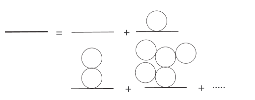
Figure 1: Scalar propagators in leading order in the large N. For vanishing expectation value of $\sigma$ these are given by a sum of cactus-type diagrams.

VI.2 Non-equilibrium Schwinger-Dyson equations

In this section we derive an exact expression for the spectrum of the magnetic field from the non-equilibrium set of Schwinger-Dyson equations.

The full non-equilibrium propagator for the photon field is obtained from the non-equilibrium effective action resulting from integrating out the charged fields, and which up to quadratic order in the photon field is given by

$$\Gamma[A^{\pm}]=\int d^{4}xd^{4}y\left\{A^{a}_{i,T}(x)\left[\partial_{\mu}\partial^{\mu}\delta^{4}(x-y)c^{ab}\delta_{ij}+\Pi^{ab}_{ij,T}(x,y)\right]A^{b}_{j,T}(y)\right\}$$ (61)

with an implicit sum over all repeated indices.

To lowest order in $\alpha$ and to leading order in the large $N$ expansion, the non-equilibrium contribution from the scalar fields to the photon polarization is given by the two diagrams shown in fig. 2.

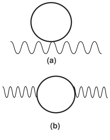
Figure 2: Photon polarization to lowest order in $\alpha$ and to leading order in the large N. The scalar loops are in terms of the scalar propagators displayed in fig.1

The tadpole diagram (a) in fig.2 gives a contribution that is local in time, thus we write the polarization

$$\Pi^{ab}_{ij,T}(x,y)={\Pi}^{tad}(t)\;c^{ab}\;\delta_{ij}\;\delta^{4}(x-y)+{\mathbf{\Pi}}^{ab}_{ij,T}(\vec{x}-\vec{y},x^{0},y^{0})\;,$$ (62)

where the form of the local (tadpole) contribution ${\Pi}^{tad}(t)$ in terms of the metric $c^{ab}$ is necessary for consistency with the form of the effective action since the kinetic term is proportional to the metric ctp and we have used spatial translational invariance. The contribution ${\mathbf{\Pi}}$ is non-local, and in equilibrium it features absorptive parts. The different components $a,b=\pm$ are defined in the same manner as the Green’s functions (51)-(53) and (56)-(58). The contribution to order $\alpha$ to the non-local part of the polarization is depicted in diagram (b) in fig.2.

The photon propagator given in eq. (50) is the inverse of the operator in the quadratic effective action above and obeys the non-equilibrium version of the Schwinger-Dyson equation ctp

$$\int d^{4}y\left[\partial_{\mu}\partial^{\mu}\delta^{4}(x-y)\;c_{ab}\;\delta_{ij}+\Pi^{ab}_{ij}(x,y)\right]\mathcal{D}^{jk}_{bc}(y,z)=\delta^{ik}\;c_{ac}\;\delta^{4}(x-z)$$ (63)

From the expressions (51)-(53) for the different components of the photon propagator it proves convenient to introduce the following combinations

$$\mathcal{D}^{C}_{ij}(x,y)=\mathcal{D}^{>}_{ij}(x,y)-\mathcal{D}^{<}_{ij}(y,x)~{}~{};~{}~{}\mathrm{antisymmetric~{}propagator}$$ (64)

$$\mathcal{D}^{R}_{ij}(x,y)=\mathcal{D}^{C}_{ij}(x,y)\;\theta(x^{0}-y^{0})~{}~{};~{}~{}\mathrm{retarded~{}propagator}$$ (65)

$$\mathcal{D}^{A}_{ij}(x,y)=\mathcal{D}^{C}_{ij}(x,y)\;\theta(y^{0}-x^{0})~{}~{};~{}~{}\mathrm{advanced~{}propagator}$$ (66)

$$\mathcal{D}^{H}_{ij}(x,y)=\mathcal{D}^{>}_{ij}(x,y)+\mathcal{D}^{<}_{ij}(y,x)~{}~{};~{}~{}\mathrm{symmetric~{}propagator}.$$ (67)

and similar definitions for the polarization $\mathbf{\Pi}$.

Using spatial translational invariance we can simplify the above form of the Schwinger-Dyson equations by introducing the spatial Fourier transform of the transverse propagators

$$\mathcal{D}^{ab}_{ij,T}(t,t^{\prime};\vec{x}-\vec{x}^{\prime})=\int\frac{d^{3}k}{(2\pi)^{3}}\;e^{i\vec{k}\cdot(\vec{x}-\vec{x}^{\prime})}\;\mathcal{P}_{ij}(\vec{k})\;{\cal D}^{ab}(t,t^{\prime};\vec{k})$$ (68)

and introducing the spatial Fourier transform of the transverse polarization tensors defined by

$${\Pi}^{ab}_{T}(t,t^{\prime};\vec{x}-\vec{x}^{\prime})=\frac{1}{2}\int\frac{d^{3}k}{(2\pi)^{3}}\;e^{i\vec{k}\cdot(\vec{x}-\vec{x}^{\prime})}\;\mathcal{P}_{ij}(\vec{k})\;\Pi^{ab}_{ij}(t,t^{\prime};\vec{k})\;.$$ (69)

We can now write down the Schwinger-Dyson equations for the transverse photon propagators. Since there are only two independent functions $D^{>,<}$ the Schwinger-Dyson equations (63) can be simplified to a set of two equations for a particular combinations of these. Some straightforward algebra leads to the following set of non-equilibrium Schwinger-Dyson equations (we have suppressed the subscript $T$ but the equations below refer to the transverse components)

$$\int dt_{1}\left[\left(\frac{d^{2}}{dt^{2}_{1}}+k^{2}+{\Pi}^{tad}(t)\right)~{}\delta(t-t_{1})+\Pi_{R}(t,t_{1};\vec{k})\right]\mathcal{D}_{R}(t_{1},t^{\prime};k)=\delta(t-t^{\prime})$$ (70)

and

$$\int dt_{1}\left[\left(\frac{d^{2}}{dt^{2}_{1}}+k^{2}+{\Pi}^{tad}(t)\right)~{}\delta(t-t_{1})+\Pi_{R}(t,t_{1};k)\right]\mathcal{D}_{H}(t_{1},t^{\prime};k)=\int dt_{1}\;\mathbf{\Pi}_{H}(t,t_{1};\vec{k}){\cal D}_{A}(t_{1},t^{\prime};k)\;.$$ (71)

with the definition

$$\Pi_{R}(t,t_{1};k)=\left[\Pi^{>}(t,t_{1};\vec{k})-\Pi^{<}(t,t_{1};k)\right]\Theta(t_{1}-t)$$ (72)

A remarkable aspect of this set of equations is that the right hand side of eq. (71), namely the inhomogeneity in the set of equations, only involves the non-local contribution to the polarization, which to lowest order in $\alpha$ is given by diagram (b) in fig. 2. This is a result of the form of the local (tadpole) contribution which is proportional to the metric $c^{ab}$. This is an important point to which we will come back later in the discussion.

The antisymmetric propagator $\mathcal{D}_{C}(t,t^{\prime\prime};k)$ is the odd solution of the homogeneous evolution equation

$$\left(\frac{d^{2}}{dt^{2}}+k^{2}+{\Pi}^{tad}(t)\right)\mathcal{D}_{C}(t,t^{\prime\prime};k)+\int_{t}^{t^{\prime\prime}}dt^{\prime}\;\Pi_{R}(t,t^{\prime},k)\;\mathcal{D}_{C}(t^{\prime},t^{\prime\prime},k)=0\;,$$ (73)

with the constraint

$$\left.\frac{\partial\mathcal{D}_{C}(t,t^{\prime},k)}{\partial t}\right|_{t^{\prime}=t}=1\;.$$ (74)

This relation guarantees the correct equal time canonical commutators.

Since the kernel of the integral equation on the left hand side of eq. (71) is the same as for the equation that defines the retarded propagator (70), the solution to eq. (71) is given by

$$\mathcal{D}_{H}(t,t^{\prime};k)=\int dt_{1}\int dt_{2}\;\mathcal{D}_{R}(t,t_{1};k)\mathbf{\Pi}_{H}(t_{1},t_{2};\vec{k})\mathcal{D}_{A}(t_{2},t^{\prime};k)+F(t,t^{\prime};k)$$ (75)

where $\mathcal{D}_{R}(t,t^{\prime};k)$ is the solution of eq. (70) and the function $F(t,t^{\prime};k)$ symmetric in $t$ and $t^{\prime}$ is a general solution of the homogeneous equation

$$\int dt_{1}\left[\left(\frac{d^{2}}{dt^{2}_{1}}+k^{2}+{\Pi}^{tad}(t)\right)~{}\delta(t-t_{1})+\Pi_{R}(t,t_{1};k)\right]F(t_{1},t^{\prime},k)=0\;.$$ (76)

The homogeneous solution $F$ can be constructed systematically and its physical significance will be discussed below.

Now are now in position to provide the final expression for the spectrum of the magnetic field. From the expression (38) and the solution found above, we find

$$S_{B}(t,k)=-ik^{2}\left.\mathcal{D}^{H}(t,t^{\prime};k)\right|_{t=t^{\prime}}$$ (77)

The expression (75) can be simplified further by taking into account the theta functions in the definitions of the retarded and the advanced (${\cal D}_{R}$ and ${\cal D}_{A}$) propagators [see eqs. (65)-(66)] as well as the antisymmetry ${\cal D}_{C}(t,t^{\prime};\vec{k})=-{\cal D}_{C}(t^{\prime},t;k)$ of $\mathcal{D}_{C}$ leading to

$$S_{B}(t,k)=i~{}k^{2}\left\{\int_{t_{0}}^{t}dt_{1}\int_{t_{0}}^{t}dt_{2}\;{\cal D}_{C}(t,t_{2};k)\;{\cal D}_{C}(t,t_{1};k)\;\mathbf{\Pi}_{H}(t_{1},t_{2};k)-F(t,t;k)\right\}\;.$$ (78)

Since the product ${\cal D}_{C}(t,t_{2};k){\cal D}_{C}(t,t_{1};k)$ is symmetric in the exchange $t_{1}\leftrightarrow t_{2}$ we can replace $\mathbf{\Pi}_{H}(t_{1},t_{2};k)$ by $2\mathbf{\Pi}_{>}(t_{1},t_{2};\vec{k})$ and write the final form of the spectrum separating, for further convenience, the contribution from the inhomogeneous and homogeneous solutions to $S_{B}$.

$$S_{B}(t,k)=S^{I}_{B}(t,k)+S^{H}_{B}(t,k)$$

$$S^{I}_{B}(t,k)=2i~{}k^{2}~{}\int_{t_{0}}^{t}dt_{1}\int_{t_{0}}^{t}dt_{2}\;{\cal D}_{C}(t,t_{2};k)\;{\cal D}_{C}(t,t_{1};k)\;\mathbf{\Pi}_{>}(t_{1},t_{2};k)$$

$$S^{H}_{B}(t,k)=-ik^{2}~{}F(t,t;k)\;.$$ (79)

where $t_{0}$ is some initial time before the phase transition and $\mathbf{\Pi}_{>}$ does not include the local tadpole contributions, it is the non-local part of the polarization.

There is an important aspect associated with the homogeneous solution $F(t,t^{\prime},k)$ and its contribution to the spectrum of generated magnetic fields $S^{B}_{H}(t,k)$. This aspect is revealed by noticing that the expectation value of the transverse gauge field $\mathcal{A}_{T}(t,k)=\langle A_{T}(t,\vec{k})\rangle$, namely the mean field obeys the same homogeneous equation of motion as $F(t,t^{\prime},k)$,

$$\int dt_{1}\left[\left(\frac{d^{2}}{dt^{2}_{1}}+k^{2}+{\Pi}^{tad}(t)\right)~{}\delta(t-t_{1})+\Pi_{R}(t,t_{1};\vec{k})\right]\mathcal{A}_{T}(t,k)=0$$ (80)

(we have suppressed the vector indices to avoid cluttering of notation).

Thus the homogeneous solution $F(t,t^{\prime},k)$ can be constructed out of the independent solutions of the mean field equations of motion (80). The main reason that we bring up this point is to highlight that the solutions to the mean-field equations of motion are only part of the contributions to the generation of magnetic fields through non-equilibrium processes. However, as it will be discussed in detail in the next section, this contribution can be neglected in the present case of non-equilibrium spinodal decomposition in many circumstances, and the term $S^{I}_{B}(t,k)$ dominates for late times.

VI.3 Electric fields:

For completeness we now address the generation of electric fields. The importance of generation of electric fields is mainly related to the question of equipartition. It is often assumed that the energy density stored in electromagnetic fields is equally partitioned between electric and magnetic field components, namely between temporal and spatial gradients. While this is usually the situation in equilibrium, it is not necessarily the case strongly out of equilibrium such as the situations envisaged in this article.

The electric field is the Hamiltonian conjugate field to the vector potential, and its transverse component is given by $E_{T}^{i}(t,\vec{k})=-\dot{A}_{T}^{i}(t,\vec{k})$, therefore the equal time correlation function of the electric field is given by

$$S_{E_{T}}(t,\vec{x})=<\dot{A}_{T}^{i}(t,\vec{x})\dot{A}_{T}^{i}(t,\vec{0}>_{c}=\partial_{t}\partial_{t^{\prime}}\left.<\frac{1}{2}\{A_{T}^{i}(t,\vec{x}),A_{T}^{i}(t^{\prime},\vec{0})\}>_{c}\right|_{t^{\prime}=t}\;.$$ (81)

where just as in the case of the magnetic field we wrote the equal time correlator as the symmetrized connected two-point correlation function.

Following the steps leading to eq. (78) for the magnetic field, and using the following identities

$$\partial_{t}{\cal D}_{R}(t,t_{1};k)=\partial_{t}{\cal D}_{C}(t,t_{1};k)\;\theta(t-t_{1}),\quad\partial_{t^{\prime}}{\cal D}_{A}(t_{2},t^{\prime};k)=-\partial_{t^{\prime}}{\cal D}_{C}(t^{\prime},t_{2};k)\;\theta(t_{2}-t^{\prime})$$

we now find

$$S_{E_{T}}(t,k)=\partial_{t}\partial_{t^{\prime}}\left\{2i\int_{t_{0}}^{t}dt_{1}\int_{t_{0}}^{t}dt_{2}\;D_{C}(t,t_{2};k)D_{C}(t^{\prime},t_{1};k)\Pi_{>}(t_{1},t_{2};k)-F(t,t^{\prime},k)\right\}_{t=t^{\prime}}$$ (82)

The number of photons produced through the non-equilibrium processes is given by

$$N(t,k)=\frac{S_{E_{T}}(t,k)+S_{B}(t,k)}{2k}-1\;,$$ (83)

after summing over the two polarization states.

The final form for the spectrum of magnetic and electric fields given by eq. (VI.2)-(82) as well as the number of photons given by eq. (83) are the main tool to compute the spectrum of electromagnetic fields generated during non-equilibrium processes and one of the main results of this article.

We emphasize that these expressions are exact and general and apply (with rather minor modifications as explained in a previous section) in the cosmological setting. They allow to study the problem of the generation of magnetic fields through non-equilibrium processes in general situations.

Furthermore, the final expressions for the spectrum of electromagnetic fluctuations (VI.2, 82) is valid more generally in spinor electrodynamics since it only involves the full polarizations and the Schwinger-Dyson equations for the correlation functions which ultimately lead to the final expressions are general.

VI.4 Spectrum of fluctuations in equilibrium

Before focusing on the study of the magnetic field generated during non-equilibrium phase transitions, it is both illuminating as well as important as a consistency check to address the case of thermal equilibrium. In this case the simplest manner to compute the spectrum is by using the imaginary time or Matsubara formulation. where the transverse photon propagator is written as kapleb

$${\cal D}^{ij}_{E}(\tau,\vec{x})=<A^{i}_{T}(\tau,\vec{x})A^{j}_{T}(\tau^{\prime},\vec{0})>=\int\frac{d^{3}k}{(2\pi)^{3}}\;e^{i{\vec{k}}\cdot{\vec{x}}}\;T\;\sum_{n\in{\mathbb{Z}}}\mathcal{P}^{ij}(\vec{k})\;{\cal D}_{T}(\omega_{n},k)\;e^{-i\omega_{n}(\tau-\tau^{\prime})}~{}~{};~{}~{}\omega_{n}=2\pi T~{}n$$ (84)

with

$${\cal D}_{T}(\omega_{n},k)=\int dk_{0}\;\frac{\rho_{T}(k,k_{0})}{k_{0}-i\omega_{n}}$$ (85)

and $\rho_{T}(k,k_{0})$ is the spectral density for transverse photons which is an odd function of $k_{0}$. The spectrum for the magnetic field is obtained from the equal time limit of the Euclidean propagator, and is therefore given by

$$S_{B}(k)=2\;k^{2}\;T\sum_{n\in{\mathbb{Z}}}{\cal D}_{T}(\omega_{n},k)\;.$$ (86)

The sum over the Matsubara frequencies can be performed using the methods described in kapleb leading to

$$S_{B}(k)=2\int d\omega\;k^{2}\;n(\omega)\;\rho_{T}(\omega,k)\;.$$ (87)

The general form of the spectral density in terms of the transverse polarization is given by kapleb

$$\rho_{T}(k,k_{0})=\frac{1}{\pi}\frac{\mathrm{Im}\Pi_{T}(k,k_{0})}{\left[k^{2}_{0}-k^{2}-\mathrm{Re}\Pi_{T}(k,k_{0})\right]^{2}+\left[\mathrm{Im}\Pi_{T}(k,k_{0})\right]^{2}}$$ (88)

The spatial and temporal Fourier transform of the retarded and advanced transverse photon propagators are given by kapleb

$$\mathcal{D}^{R}_{ij}(k,\omega)=\mathcal{P}_{ij}(k)\mathcal{D}^{R}(k,\omega)~{}~{};~{}~{}\mathcal{D}^{R}(k,\omega)=\frac{1}{-\omega^{2}+k^{2}+\mathrm{Re}\Pi_{T}(k,\omega)+i\;\mathrm{Im}\Pi_{T}(k,\omega)}$$ (89)

(90)

$$\mathcal{D}^{A}_{ij}(k,\omega)=\mathcal{P}_{ij}(\vec{k})\mathcal{D}^{A}(k,\omega)~{}~{};~{}~{}\mathcal{D}^{A}(k,\omega)=\frac{1}{-\omega^{2}+k^{2}+\mathrm{Re}\Pi_{T}(k,\omega)-i\;\mathrm{Im}\Pi_{T}(k,\omega)}$$ (91)

We are now in conditions to establish contact with the non-equilibrium result of the first section. In equilibrium the polarization and the propagators are functions of the time differences and we can then take the Fourier transform in time of $\mathcal{D}_{H}(t,t^{\prime},k)$ given by eq. (75)

$$\mathcal{D}_{H}(k,\omega)=\mathcal{D}_{R}(k,\omega)\left[\mathbf{\Pi}_{>}(k,\omega)+\mathbf{\Pi}_{<}(k,\omega)\right]\mathcal{D}_{A}(k,\omega)+F(k,\omega)$$ (92)

where we have explicitly written $\mathbf{\Pi}$ in terms of $\mathbf{\Pi}_{<,>}$. In equilibrium the detailed balance (or KMS) condition relates these components of the polarization to the imaginary partkapleb

$$\mathbf{\Pi}_{>}(k,\omega)=\frac{i}{\pi}[1+n(\omega)]\;\mathrm{Im}\mathbf{\Pi}(k,\omega)~{}~{};~{}~{}\mathbf{\Pi}_{<}(k,\omega)=\frac{i}{\pi}\;n(\omega)\;\mathrm{Im}\mathbf{\Pi}(k,\omega)$$ (93)

with $n(\omega)$ being the Bose-Einstein distribution function.

Furthermore, the Fourier transform of the homogeneous solution $F(t,t^{\prime},k)$ obeys the Fourier transform of eq. (76) namely

$${\cal D}_{R}^{-1}(\omega,k)\;F(\omega,k)=0$$ (94)

Combining all the above ingredients and using the fact that $\mathrm{Im}\mathbf{\Pi}(k,\omega)$ is an odd function of $\omega$kapleb we are led to the conclusion that eq. (77) for the spectrum becomes

$$S_{B}(k)=\int d\omega\;\left\{2\;k^{2}\;n(\omega)\;\rho_{T}(\omega,k)+k^{2}\;F(\omega,k)\right\}$$ (95)

with $\rho_{T}(\omega,k)$ given by eq. (88).

This result differs from that obtained via the equilibrium propagator eq. (87) by the contribution of the homogeneous solution $F$.

In order to understand the source of the discrepancy between the two formulations, namely the contribution of the homogeneous solution $F(k,\omega)$, let us focus on the defining equation for $F(k,\omega)$ (94).

In order for a non-vanishing solution to this equation to exist, from the expression for $\mathcal{D}_{R}(k,\omega)$ we infer that

$$\omega^{2}-k^{2}-\mathrm{Re}\Pi_{T}(k,\omega)=0$$ (96)

$$\mathrm{Im}\Pi_{T}(k,\omega)=0$$ (97)

Eq. (96) determines the dispersion relation of quasiparticles and eq. (97) determines that these quasiparticles must have zero width, i.e, the solutions of the homogeneous equations are propagating quasiparticles with zero width and a dispersion relation given by (96). The homogeneous solution is therefore

$$F(k,\omega)\propto\delta(\omega^{2}-k^{2}-\mathrm{Re}\Pi_{T}(k,\omega))$$ (98)

In a non-perturbative resummation of the Dyson series for the propagators and the spectral density, the limit when $\mathrm{Im}\Pi_{T}\rightarrow 0^{\pm}$ leads to

$$\rho_{T}\rightarrow\mp\delta(\omega^{2}-k^{2}-\mathrm{Re}\Pi_{T}(k,\omega))$$ (99)

and we recognize in this case that the possible contributions of the homogeneous solutions are accounted for in the expressions (88) and arise from the propagating states, and to zeroth order account for the contribution to the spectrum of the magnetic field from free photons.

However, in a perturbative expansion perturbation theory is only reliable away from the single particle poles in the propagator and the limit $\mathrm{Im}\Pi_{T}\rightarrow 0^{\pm}$ will miss the contribution from the isolated poles. The homogeneous solution $F(k,\omega)$ gives the required contribution, thus guaranteeing the consistency of the perturbative expansion. Thus while the homogeneous solution $F$ must be included in a perturbative calculation of the spectrum, it will be accounted for in a non-perturbative computation that includes a Schwinger-Dyson resummation for the full propagator and should not be included in the computation of the spectrum.

In a plasma the true degrees of freedom are quasiparticles, in particular for the power spectrum of magnetic and transverse electric fields, the important degrees of freedom are transverse plasmons. In the hard thermal loop approximationkapleb the transverse plasmons contribute to the spectral density $\rho_{T}(k,\omega)$ a pole term of the form $Z_{T}(k)[\delta(\omega-\omega_{p}(k))-\delta(\omega+\omega_{p}(k)]$ with $\omega_{p}(k)$ being the plasmon dispersion relationkapleb with $\omega_{p}(0)=eT/3$. For $k\gg eT,\;\omega_{p}(k)\sim k~{};~{}Z_{T}\sim 1/2k$ and we recover the power spectrum of free field theory. However for $k\lesssim eT$ the power spectrum of the magnetic field reveals the presence of collective degrees of freedom, $S_{B}(k)\sim kZ_{T}(k)[1+2\,n(\omega_{p}(k)]$ for $e^{2}T\leq k\leq eT$.

For ultrasoft frequency and momenta $k,\omega\ll eT$ which is the case of relevance for the cosmological case, the effective low energy form of the gauge field (transverse) propagator (well below the plasmon pole) is

$${\cal D}(k,\omega)\simeq\frac{1}{\omega^{2}-k^{2}-i\sigma\omega}$$ (100)

leading to the small frequency, long-wavelength form of the spectral density

$$\rho_{T}(k,\omega)\simeq\frac{1}{\pi}\frac{\sigma\;\omega}{(\omega^{2}-k^{2})^{2}+(\sigma\omega)^{2}}\;.$$ (101)

Therefore, for $\omega\ll\sigma$

$$k^{2}\;n(\omega)\;\rho_{T}(k,\omega)\simeq\frac{T}{\pi}\frac{\Gamma}{\omega^{2}+\Gamma^{2}}~{}~{};~{}~{}\Gamma\equiv\frac{k^{2}}{\sigma}\;.$$ (102)

Thus for long wavelengths $k\ll\sigma\approx T/\alpha$ the spectral density features a pole at zero frequency leading to a long-wavelength power spectrum

$$S_{B}(k\ll\sigma)=T\;,$$ (103)

coming from the first term in eq.(95).

The plasmon pole contributes to $S_{B}(k)$ through the homogeneous solution $F$ in eq.(95) yielding,

$$S_{Bplasmon}\simeq\frac{k^{2}}{\omega_{p}(0)}[1+2n(\omega_{p}(0)]\sim\frac{2k^{2}T}{\omega^{2}_{p}(0)}\sim\frac{k^{2}}{e^{2}T}$$ (104)

where we have used the long-wavelength limit of the dispersion relation $\omega_{p}(k)$ and residue $Z_{T}(k)$kapleb . The contribution (104) is clearly much smaller than (103) in the long-wavelength limit $k\ll eT$. Hence, the magnetic field power spectrum in equilibrium is $S_{B}(k)\simeq T$.

Having clarified the role of the homogeneous solution and the form of the power spectrum within the more familiar equilibrium setting, we return to the non-equilibrium situation.

VII Spectrum out of equilibrium

The set of equations for the spectra of magnetic and electric fields (VI.2)-(82) is exact and only involves the transverse polarization from which the full propagator and inhomogeneous and homogeneous solutions are obtained. Obviously in order to make progress and obtain an estimate for magnetic and electric field generation one has to make approximations. In what follows we will obtain the spectra for magnetic and electric fields to lowest order in $\alpha$ and to leading order in large $N$.

To this order the tadpole (local) and bubble (non-local) contribution to the polarization are given respectively by diagrams (a) and (b) in fig. 2. Their explicit expressions are given by

$$\Pi^{tad}(t) = -ie^{2}N\int\frac{d^{3}q}{(2\pi)^{3}}\;{G}_{>}(t,t,q)\;,$$ (105)

$$\Pi_{ij,>}(t_{1},t_{2},\vec{k}) = ie^{2}N\int\frac{d^{3}q}{(2\pi)^{3}}\;(2q_{i}+k_{i})\;(2q_{j}+k_{j})\;G_{>}(t_{1},t_{2},q)\;G_{>}(t_{1},t_{2},|\vec{q}+\vec{k}|)\;.$$ (107)

which leads to the transverse components

$$\Pi_{>}(t_{1},t_{2},k)=2ie^{2}N\int\frac{d^{3}q}{(2\pi)^{3}}\;q^{2}\;(1-\cos^{2}\theta)~{}G_{>}(t_{1},t_{2},q)\;G_{>}(t_{1},t_{2},|\vec{q}+\vec{k}|)\;,$$ (108)

(109)

$$\Pi_{<}(t_{1},t_{2},k)=\Pi_{>}(t_{2},t_{1},k)\;.$$ (110)

where $\cos\theta\equiv{\hat{q}}\cdot{\hat{k}}$. The scalar propagator $G_{>}(t,t^{\prime})$ in terms of the mode functions $f_{q}(t)$ that satisfy the evolution equations (18) is given by [see eq. (59)],

$$G_{>}(t_{1},t_{2};k)=\frac{i}{2}\left[(1+n_{k})f_{k}(t_{1})f_{k}^{*}(t_{2})+n_{k}f_{k}^{*}(t_{1})f_{k}(t_{2})\right]\;.$$ (111)

and we assumed that before the phase transition the scalar fields have occupation $n_{k}$ (obviously this assumption can be relaxed straightforwardly).

From these expressions we can obtain a reliable estimate of the non-equilibrium effects in the polarization. For intermediate times after the phase transition, when the dynamics is dominated by the spinodal instabilities and before the non-linearities in the scalar field evolution are important, the long-wavelength mode functions are approximately given by eq.(27).

Near the end of the phase transition for $t\sim t_{nl}\approx\frac{1}{2\,\mu}\ln\left(\frac{1}{\lambda}\right)$ the leading order time dependence of the scalar Green’s functions is then approximately given by

$$G_{>}(t,t^{\prime},k)_{t,t^{\prime}\sim t_{nl}}\approx e^{\mu(t+t^{\prime})}\approx\frac{1}{\lambda}$$ (112)

which allows us to estimate the order of magnitude of the different terms in the polarization. For the tadpole contribution (local term) we find

$$\Pi^{tad}(t)_{t\sim t_{nl}}\approx e^{2}~{}\mu^{2}\;e^{2\mu t}\approx e^{2}\;\frac{\mu^{2}}{\lambda}+{\cal O}\left(\frac{1}{\sqrt{\lambda}}\right)$$ (113)

This estimate is consistent with the fact that the tadpole contribution is $e^{2}<\Phi\Phi>$ and near the end of the phase transition the mean square root fluctuations of the scalar field probe the vacuum state, namely $<\Phi^{2}>\sim\mu^{2}/\lambda$. Similarly, we find for $k\ll\mu$,

$$\Pi_{>}(t,t^{\prime},k)_{t\sim t_{nl}}\buildrel t\sim t_{nl}\over{=}-\frac{i\;e^{2}N\sqrt{\mu}}{128\;\pi^{\frac{3}{2}}}\;\left(1+\frac{M^{2}}{\mu^{2}}\right)^{2}\;\frac{e^{(t+t^{\prime})(2\mu-\frac{k^{2}}{4\mu})}}{(t+t^{\prime})^{\frac{5}{2}}}\left[1+{\cal O}\left(\frac{1}{t}\right)\right]\;,$$ (114)

which for $t\sim t^{\prime}\sim t_{nl}$ is of the order $1/\lambda^{2}$.

Since the retarded polarization given by eq. (72) is antisymmetric in the time arguments the leading contribution given by (114) above, actually cancels since $\Pi_{<}(t,t^{\prime},k)=\Pi_{>}(t^{\prime},t,k)$. A detailed analysis (see ref. Boyanovsky:1999jh ) reveals that the retarded non-local part $\Pi_{R}$ is of the same order as the tadpole contribution, namely

$$\Pi_{R}\approx e^{2}~{}\frac{\mu^{2}}{\lambda}$$ (115)

and that in fact at long times there is an exact cancellation between the two terms for $k\approx 0$ in Minkowski space-time. This is in agreement with the equilibrium result of a vanishing magnetic masskapleb .

VII.1 Spinodal decomposition from a vacuum state

To understand the order of magnitude of the generated magnetic fields and to gain insight into the main features of the non-equilibrium processes, we now study the situation of spinodal decomposition from an initial vacuum state. This corresponds to considering an initial state in which the $\sigma$ field rolls down the potential hill while the fluctuations of the charged fields are in the vacuum state at the initial time. The dynamics of the scalar field in this case has been studied thoroughly analytically and numerically in references boysinglee ; eri95 ; eri97 ; destri to which the reader is referred.

For times smaller than or of the order of the nonlinear time (30) we can evaluate the tadpole diagram (105) using eqs.(111) and (27) with the result,

$$\Pi^{tad}(t)=\frac{e^{2}\,N}{64\,\pi^{\frac{3}{2}}}\;(\mu^{2}+M^{2})\;\sqrt{\frac{M}{\mu}}\;(1+2\,n_{0})\;\frac{e^{2\,\mu\,t}}{(M\,t)^{\frac{3}{2}}}\left[1+{\cal O}\left(\frac{1}{t}\right)\right]\;.$$ (116)

Let us now consider the retarded bubble diagram

$$\Pi_{R}(t_{1},t_{2};k)=-4e^{2}N\int\frac{d^{3}q}{(2\pi)^{3}}\;q^{2}\;(1-\cos^{2}\theta)~{}\mbox{Im}\left[G_{>}(t_{1},t_{2},q)\;G_{>}(t_{1},t_{2},|\vec{q}+\vec{k}|)\right]\;\theta(t_{2}-t_{1})$$ (117)

where we used eq.(72) and (108).

We are interested in the generation of long-wavelength magnetic fields with $k\ll\mu$. The bubble diagram $\Pi_{R}(t_{1},t_{2};k)$ takes the form,

$$\Pi_{R}(t_{1},t_{2};k) = -4\int_{0}^{+\infty}\frac{q^{4}\,dq}{(2\,\pi)^{2}}\;\int_{-1}^{+1}dx\;(1-x^{2})\;\mbox{Im}\left[G_{>}(t_{1},t_{2},q)\;G_{>}(t_{1},t_{2},|{\vec{q}}+{\vec{k}}|)\right]\;\theta(t_{2}-t_{1})$$ (118)

$$= \int_{0}^{+\infty}\frac{q^{4}\,dq}{(2\,\pi)^{2}}\;\int_{-1}^{+1}dx\;(1-x^{2})\;\mbox{Im}\left[f_{q}(t_{1})\;{\bar{f}}_{q}(t_{2})f_{|{\vec{q}}+{\vec{k}}|}(t_{1})\;{\bar{f}}_{|{\vec{q}}+{\vec{k}}|}(t_{2})\right]\;\theta(t_{2}-t_{1})\;.$$ (120)

where $x\equiv{\hat{q}}\cdot{\hat{k}}$ and we set the temperature equal to zero. For times smaller or of the order of the nonlinear time (30) we can evaluate this bubble diagram using eq.(26) for the mode functions. This gives for $\mu\,t\gg 1$, fixed $t^{\prime}$ and $k\ll\mu$,

$$\mbox{Im}\left[f_{q}(t)\;{\bar{f}}_{q}(t^{\prime})f_{|{\vec{q}}+{\vec{k}}|}(t)\;{\bar{f}}_{|{\vec{q}}+{\vec{k}}|}(t^{\prime})\right]\buildrel\mu\,t\gg 1,k\ll\mu\over{=}e^{t(2\,\mu-\frac{q^{2}}{\mu})}\left[2\;|a_{q}^{2}|\;\mbox{Im}(a_{q}^{2})\;e^{-t(\frac{k^{2}}{2\mu}+\frac{kqxt}{\mu})}+\mbox{Im}(a_{q}^{4})\;e^{-t^{\prime}(2\,\mu-\frac{q^{2}}{\mu})}\;e^{-(t-t^{\prime})(\frac{k^{2}}{2\mu}+\frac{kqxt}{\mu})}\right]\;.$$

Calculating now the $q$ integrals in eq.(118) for $\mu\,t\gg 1$ yields

$$\Pi_{R}(t,t^{\prime};k)\buildrel\mu\,t\gg 1,k\ll\mu\over{=}-e^{2}\,N\,\frac{(\mu^{2}+M^{2})}{16\,M\,\sqrt{\mu}\,\pi^{\frac{3}{2}}}\;\frac{e^{t(2\,\mu-\frac{k^{2}}{4\mu})}}{t^{\frac{5}{2}}}\left[1+2\,e^{-t^{\prime}(2\,\mu-\frac{k^{2}}{4\mu})}\right]\;.$$ (121)

where we used eq.(26).

Using eqs.(116) and (121), the photon evolution equation (73) takes the form

$$\left(\frac{d^{2}}{dt^{2}}+k^{2}+e^{2}\;C^{2}\;\frac{e^{2\,\mu\,t}}{t^{\frac{3}{2}}}\right)\mathcal{D}_{C}(t,t^{\prime\prime};k)-\frac{e^{t(2\,\mu-\frac{k^{2}}{4\mu})}}{t^{\frac{5}{2}}}\;e^{2}\;L(t,t^{\prime\prime})=0\;,$$ (122)

where

$$C^{2} = \frac{N}{64\,\pi^{\frac{3}{2}}}\;\frac{\mu^{2}+M^{2}}{M\;\sqrt{\mu}}$$ (123)

$$L(t,t^{\prime\prime}) = \frac{N(\mu^{2}+M^{2})}{16\,M\,\sqrt{\mu}\,\pi^{\frac{3}{2}}}\;\int_{t}^{t^{\prime\prime}}dt^{\prime}\;\left[1+2\,e^{-t^{\prime}(2\,\mu-\frac{k^{2}}{4\mu})}\right]\mathcal{D}_{C}(t^{\prime},t^{\prime\prime};k)$$ (125)

Eq.(122) is valid for times larger than $1/\mu$ and smaller or approaching the nonlinear time $t_{nl}$ [see eq.(30)]. It can be considered an inhomogeneous equation for $\mathcal{D}_{C}(t^{\prime},t^{\prime\prime};k)$, where the inhomogeneity is to be determined self-consistently.

Let us first consider the homogeneous version of equation (122),

$$\left(\frac{d^{2}}{dt^{2}}+k^{2}+e^{2}\;C^{2}\;\frac{e^{2\,\mu\,t}}{t^{\frac{3}{2}}}\right)\phi(t)=0$$ (126)

This equation has as general solution for $\mu\,t\gg 1$ and $k\ll\mu$

$$\phi(t)\buildrel\mu\,t\gg 1\over{=}t^{\frac{3}{8}}\;e^{-\frac{\mu\,t}{2}}\left[A\;\cos\left(\frac{e\,C}{\mu\;t^{\frac{3}{4}}}\;e^{\mu\,t}\right)+B\;\sin\left(\frac{e\,C}{\mu\;t^{\frac{3}{4}}}\;e^{\mu\,t}\right)\right]$$ (127)

where $A$ and $B$ are arbitrary constants.

In order to solve eq.(122) we use the Green function of eq.(126)

$$\left(\frac{d^{2}}{dt^{2}}+k^{2}+e^{2}\;C^{2}\;\frac{e^{2\,\mu\,t}}{t^{\frac{3}{2}}}\right)G(t,t^{\prime})=\delta(t-t^{\prime})$$

that can be written explicitly as,

$$G(t,t^{\prime})=-\frac{1}{e\,C}\;(t\,t^{\prime})^{\frac{3}{8}}\;e^{-\frac{\mu}{2}(t+t^{\prime})}\sin\left(\frac{e\,C}{\mu\;t_{<}^{\frac{3}{4}}}\;e^{\mu\,t_{<}}\right)\;\cos\left(\frac{e\,C}{\mu\;t_{>}^{\frac{3}{4}}}\;e^{\mu\,t_{>}}\right)$$ (128)

We can thus write the antisymmetric solution of eq.(122) as follows,

$$\mathcal{D}_{C}(t,t^{\prime\prime};k)=\frac{1}{e\,C}\;(t\,t^{\prime})^{\frac{3}{8}}\;e^{-\frac{\mu}{2}(t+t^{\prime})}\sin\left[\frac{e\,C}{\mu}\left(\frac{e^{\mu\,t}}{t^{\frac{3}{4}}}-\frac{e^{\mu\,t^{\prime\prime}}}{t^{\prime\prime\frac{3}{4}}}\right)\right]+e^{2}\;\int dt^{\prime}\left[\;G(t,t^{\prime})\;\frac{e^{t^{\prime}(2\,\mu-\frac{k^{2}}{4\mu})}}{t^{\prime\frac{5}{2}}}\;L(t^{\prime},t^{\prime\prime})-(t\leftrightarrow t^{\prime\prime})\right]$$ (129)

The first term provides an antisymmetric solution of eq.(126) which is normalized according to eq.(74). The second term comes from the inhomogeneity in eq.(122).

For $t\sim t_{nl}$ the first term is of the order $\lambda^{\frac{1}{4}}$. Let us now compute the second term which will dominate in such regime. From the explicit form of $L(t^{\prime},t^{\prime\prime})$ (123) and the solution for $\mathcal{D}_{C}(t,t^{\prime\prime};k)$ given by eqn. (129) it is clear that $L(t^{\prime},t^{\prime\prime})$ is a slowly varying function of its arguments. In particular we can set $t^{\prime}=t_{nl}$ and take $L(t^{\prime},t^{\prime\prime})\sim L(t_{nl},t^{\prime\prime})$ outside of the integral.

Using the results given in eqs.(128) and (129) we find the following result,

$$\int dt^{\prime}\;G(t,t^{\prime})\;\frac{e^{2\,\mu\,t^{\prime}}}{t^{\prime\frac{5}{2}}}=\frac{e^{-\frac{k^{2}\,t}{4\,\mu}}}{e^{2}\;C^{2}\;t^{1+\frac{3\,k^{2}}{16\,\mu^{2}}}}$$ (130)

for $1/\mu\ll t<t_{nl}$. We find at $t=t_{nl}$,

$$\int dt^{\prime}\;G(t_{nl},t^{\prime})\;\frac{e^{2\,\mu\,t^{\prime}}}{t^{\prime\frac{5}{2}}}=\frac{e^{-\frac{k^{2}\,t_{nl}}{4\,\mu}}}{2\;e^{2}\;C^{2}\;t_{nl}^{1+\frac{3\,k^{2}}{16\,\mu^{2}}}}$$ (131)

where we have neglected rapidly oscillating phases.

We finally get collecting all factors and taking into account that $L(t^{\prime},t^{\prime\prime})$ varies slowly with $t^{\prime}$ compared with $e^{2\,\mu\,t^{\prime}}$,

$$\mathcal{D}_{C}(t,t^{\prime\prime};k)\buildrel t_{nl}>t\gg 1/\mu\over{=}\frac{L(t_{nl},t^{\prime\prime})}{C^{2}\;t^{1+\frac{3\,k^{2}}{16\,\mu^{2}}}}\;e^{-\frac{k^{2}\,t}{4\,\mu}}$$ (132)

and

$$\mathcal{D}_{C}(t_{nl},t^{\prime\prime};k)=\frac{L(t_{nl},t^{\prime\prime})}{2\;C^{2}\;t_{nl}^{1+\frac{3\,k^{2}}{16\,\mu^{2}}}}\;e^{-\frac{k^{2}\,t_{nl}}{4\,\mu}}$$ (133)

Notice that $e^{2}$ cancels in eqs.(132) and (133) since both integrals (130) and (131) are proportional to $e^{-2}$ and the inhomogeneity in eq.(122) is proportional to $e^{2}$. Therefore, $\mathcal{D}_{R}(t,t^{\prime},k)$ is of the order $e^{0}$ for $1/\mu\ll t\leq t_{nl},\;k\ll\mu$ and fixed $t^{\prime}$.

We thus obtain for the magnetic field spectrum in the long wavelength limit from eq.(VI.2),

$$S_{B}(t_{nl},k)\buildrel k\ll\mu\over{=}2ik^{2}\;\int_{t_{0}}^{t_{nl}}dt_{1}\int_{t_{0}}^{t_{nl}}dt_{2}\;{\cal D}_{C}(t_{nl},t_{2};k)\;{\cal D}_{C}(t_{nl},t_{1};k)\;\mathbf{\Pi}_{>}(t_{1},t_{2};k)$$ (134)

and we used the fact that the homogeneous contribution $S^{H}_{B}(t,k)$ in eq.(VI.2) can be neglected for $t=t_{nl}$ according to eq.(127). We can now insert eq.(133) for $\mathcal{D}_{C}(t_{nl},t^{\prime\prime};k)$ into eq.(134). The fastly growing factors $e^{2\,\mu\,t}$ in eq.(114) combine with powers of $t$ to give near $t_{nl}\sim\frac{1}{2\mu}\log\frac{1}{\lambda}$ a factor

$$\frac{e^{-\frac{k^{2}\,t_{nl}}{\mu}}}{\lambda^{2}\;\left(\log\frac{1}{\lambda}\right)^{\frac{3}{2}+\frac{3\,k^{2}}{8\,\mu^{2}}}}$$

dominating the integrals. We used here that $L(t_{nl},t)\sim(t_{nl}-t)^{2}$ for $t\sim t_{nl}$. This relation follows from the fact that ${\cal D}_{C}(t,t^{\prime};k)\buildrel t\to t^{\prime}\over{=}(t-t^{\prime})$ due to eq.(74) and using the relation (123) for $t\to t^{\prime\prime}$.

Performing the integrals in eq.(134) for $t=t_{nl}$ we obtain neglecting corrections in $1/\ln\frac{1}{\lambda}$,

$$S_{B}(t_{nl},k)\buildrel k\ll\mu\over{=}\frac{k^{2}}{\mu}\;\frac{N\;e^{2}}{\lambda^{2}\;\left(\log\frac{1}{\lambda}\right)^{\frac{3}{2}+\frac{3\,k^{2}}{8\,\mu^{2}}}}\frac{1}{2^{9}\;\pi^{\frac{3}{2}}}\;\left(1+\frac{M^{2}}{\mu^{2}}\right)^{2}\;e^{-\frac{k^{2}\,t_{nl}}{\mu}}\left[1+{\cal O}\left(\frac{1}{\log\frac{1}{\lambda}}\right)\right]$$ (135)

where we used eq.(123).

We read in eq.(135) the correlation length of the scalar field at the nonlinear timeboysinglee ,

$$\xi(t_{nl})=2\;\sqrt{\frac{t_{nl}}{\mu}}\simeq\frac{2}{\mu}\,\sqrt{\ln\frac{1}{\lambda}}\;,$$ (136)

The expression (135) for the spectrum of the magnetic field clearly reveals that the correlation length of the magnetic field tracks that of the scalar field during the stage of spinodal decomposition. This result is intuitively clear since the magnetic field is generated by the long-wavelength spinodal instabilities corresponding to the formation of correlated domains that grow in time during the spinodal regime as $\xi(t)\approx\sqrt{2t/\mu}$ boysinglee . From $S_{B}(t,k)$ we can extract the magnetic energy density in long-wavelength scales equal to or larger than $L$ through eq.(46).

The energy density on scales $\geq L$ given by eq. (46) can be computed in closed form in the limits $L\gg\xi(t_{nl})$ or $1/\mu\ll L\ll\xi(t_{nl})$ using eq.(135). We find

$$\frac{\rho_{B}(L)}{\rho_{\gamma}}=\frac{N\;e^{2}}{\lambda^{2}\;\log^{4}\frac{1}{\lambda}}\;\frac{1}{2^{11}\;\sqrt{2}\;5\pi^{5}}\;\left(1+\frac{M^{2}}{\mu^{2}}\right)^{2}\;\left(\frac{\mu}{T}\right)^{4}\;,\quad 1/\mu\ll L\ll\xi(t_{nl})\;,$$ (137)

and

$$\frac{\rho_{B}(L)}{\rho_{\gamma}}=\frac{N\;e^{2}}{\lambda^{2}\;\log^{\frac{3}{2}}\frac{1}{\lambda}}\;\frac{3}{32\;\sqrt{\pi}}\;\left(1+\frac{M^{2}}{\mu^{2}}\right)^{2}\;\frac{1}{\mu\,L}\;\frac{1}{\left(L\,T\right)^{4}}\;,\quad L\gg\xi(t_{nl})$$ (138)

for the energy on macroscopic scales . This latter can be interpreted as energy on magnetic fields coherent on scales of the order or bigger than $L$. We see that large scale magnetic fields are strongly suppressed as $L^{-5}$.

We now compute the spectrum of the electric field from eq.(82). We evaluate the integrals is eq.(82) by the same lines as the eq.(134) using eqs.(132) and (114) for $D_{C}(t,t^{\prime};k)$ and $\Pi_{>}(t_{1},t_{2};k)$, respectively. We find that the end-point near $t_{nl}$ dominates the integrals with the result

$$S_{E_{T}}(0,t_{nl})\sim\frac{N\;e^{2}\;\mu}{\lambda^{2}}\;\frac{1}{\sqrt{\log\frac{1}{\lambda}}}$$ (139)

and therefore,

$$\frac{S_{B}(k,t_{nl})}{S_{E_{T}}(k,t_{nl})}\sim\frac{k^{2}}{\mu^{2}}\;\frac{1}{\log\lambda}$$ (140)

Thus we see that for long-wavelengths $k\ll\mu$ the strength of the electric fields generated are much larger than those of the magnetic fields. This result clearly indicates a violation of equipartition as a consequence of the non-equilibrium generation of electromagnetic fields. If spinodal decomposition occurs from a vacuum state, namely the $\sigma$ field rolls from the top of the potential and the charged fields are in a vacuum state, the non-equilibrium processes generate mainly electric photons.

VII.2 Spinodal decomposition in a high temperature plasma

We now study the case of a rapid (quenched) phase transition from an initial high temperature phase to a final low temperature phase. Before the phase transition the system is in (local) thermodynamic equilibrium at a temperature $T>>T_{c}$ with $T_{c}\propto\mu/\sqrt{24\lambda}$ and the long-wavelength $k\ll T$ modes acquire a thermal mass kapleb

$$m_{T}=\sqrt{\frac{\lambda}{24}}~{}T.$$ (141)

The occupation number of a mode of momentum $q$ is given by the Bose-Einstein distribution function

$$n(q)=\frac{1}{e^{\frac{\omega(q)}{T}}-1}~{}~{};~{}~{}\omega(q)=\sqrt{q^{2}+m^{2}_{T}}$$ (142)

Short wavelength modes with momenta $q>>\lambda T$ remain in local thermodynamic equilibrium during the (quenched) phase transition, while long-wavelength modes undergo critical slowing down critslowdown , freeze out and fall out of equilibrium. These long-wavelength modes will undergo spinodal decomposition and their mode functions for $\mu^{-1}<t\leq t_{nl}$ will grow as (see eq. (26)

$$f_{q}(t)\simeq-i\;a_{q}\;e^{[\mu-q^{2}/(2\mu)]t},\quad a_{q}\sim a_{0}\sim\frac{\sqrt{m_{T}}}{2\mu}\;.$$ (143)

since for $T^{2}\gg T_{c}^{2}=\frac{24}{\lambda}\mu^{2}$ it follows that $m_{T}\gg\mu$.

In a high temperature plasma, charge fluctuations lead to a large conductivity in the medium. In equilibrium the conductivity is obtained from the imaginary part of the photon polarization and it is dominated by particles of momenta $p\sim T$ in the loop with exchange of photons of momenta $eT<k\ll T$ baym ; yaffe . The Drude conductivity for an ultrarelativistic plasma at temperature $T$ much larger than the mass of the charged fields (in this case $m_{T}\sim\sqrt{\lambda}T\ll T$) is given by

$$\sigma_{c}=\frac{e^{2}\mathcal{N}(T)\;\tau}{T}$$ (144)

with $\mathcal{N}(T)\propto T^{3}$ is the number of particles plus antiparticles in the plasma and $\tau$ is the transport relaxation time. A naive estimate based on the scattering amplitude with the exchange of photons or charged particles with momenta $p\sim T$ would indicate that $\tau^{-1}\sim\mathcal{N}(T)~{}\alpha^{2}/T^{2}\sim\alpha^{2}T$ (with $\alpha^{2}/T^{2}$ the typical cross section from the exchange of a particle with $p\sim T$) and would lead to a Drude conductivity of the form

$$\sigma\sim\frac{T}{\alpha}$$ (145)

However, a careful analysis including Debye (electric) and dynamical (magnetic) screening via Landau damping leads to the conclusion that the conductivity is given by baym ; yaffe

$$\sigma=\frac{\mathcal{C}\;N\;T}{\alpha\ln\left[\frac{1}{\alpha{N}}\right]}$$ (146)

with $N$ the number of charged fields and $\mathcal{C}\sim\mathcal{O}(1)$. Thus we consider separately the contributions to the photon polarization from loop momenta in the two very different regimes: a) the hard momenta $p\sim T\gg\mu$ correspond to charge fluctuations that are always in local thermodynamic equilibrium, b) the soft momenta $p\ll\mu$ fall out of equilibrium and undergo long-wavelength spinodal instabilities. The contribution from hard momenta will lead to a large equilibrium conductivity in the medium, while the contribution to the polarization from soft momenta will contain all the non-equilibrium dynamics that lead to the generation of electromagnetic field fluctuations.

As the instabilities during the phase transition develop, the fluctuations of the charged fields will generate non-equilibrium fluctuations in the long-wavelength components of the electric and magnetic fields and the ensuing generation of long-wavelength magnetic fields. However, the large conductivity of the medium will hinder the generation of electromagnetic fluctuations, hence the conductivity must be fully taken into account to assess the spectrum of the magnetic and electric fields generated during the non-equilibrium stage.

In equilibrium the long-wavelength and low frequency limit ($k,\omega\rightarrow 0$) of the spatial and temporal Fourier transform of the transverse polarization is given by

$$\Pi_{T}(k,\omega)=i\omega\sigma$$ (147)

Thus we write for the full transverse polarization for long-wavelength electromagnetic fields

$$\Pi_{T}(t,t^{\prime},k)=\sigma\;\frac{d}{dt^{\prime}}\delta(t-t^{\prime})+\Pi_{noneq}(t,t^{\prime},k)$$ (148)

with $\Pi_{noneq}(t,t^{\prime},k)$ the contribution from the spinodally unstable long-wavelength modes given by equations (105). Our strategy is to obtain the non-equilibrium contribution to the spectrum of electromagnetic fields to lowest order in $\alpha$ but treating the conductivity exactly.

The zeroth order propagators are now obtained by considering the contribution from the conductivity to the equations of motion, the relevant retarded, advanced and symmetric transverse correlators obey

$$\left[\frac{d^{2}}{dt^{2}}+k^{2}+\sigma\frac{d}{dt}\right]\mathcal{D}^{(0)}_{R}(t,t^{\prime},k)=\delta(t-t^{\prime})~{}~{};~{}~{}\mathcal{D}_{R}(t,t^{\prime})=0~{}~{}\mathrm{for}~{}t<t^{\prime}$$ (149)

$$\left[\frac{d^{2}}{dt^{2}}+k^{2}+\sigma\frac{d}{dt}\right]\mathcal{D}^{(0)}_{A}(t,t^{\prime},k)=\delta(t-t^{\prime})~{}~{};~{}~{}\mathcal{D}_{A}(t,t^{\prime})=0~{}~{}\mathrm{for}~{}t>t^{\prime}$$ (150)

$$\left[\frac{d^{2}}{dt^{2}}+k^{2}+\sigma\frac{d}{dt}\right]\mathcal{D}^{(0)}_{H}(t,t^{\prime},k)=0$$ (151)

Since $\sigma\sim T/\alpha$ and in the initial state $T>T_{c}\sim\mu/\sqrt{\lambda}$ then for time scales in the intermediate regime $\mu^{-1}<t<t_{nl}$ it is clear that $t\gg\sigma^{-1}$.

For $k\ll\sigma$ and $t\gg 1/\sigma$ (when we can neglect the second order time derivatives in (149-151)) we find

$$\mathcal{D}^{(0)}_{R}(t,t^{\prime},k)=\frac{e^{-\frac{k^{2}}{\sigma}(t-t^{\prime})}}{\sigma}\;\theta(t-t^{\prime})\quad,\quad\mathcal{D}^{(0)}_{A}(t,t^{\prime},k)=-\frac{e^{-\frac{k^{2}}{\sigma}(t-t^{\prime})}}{\sigma}\;\theta(t^{\prime}-t)$$ (152)

$$\mathcal{D}^{(0)}_{H}(t,t^{\prime},k)=i\;\frac{e^{-\frac{k^{2}}{\sigma}(t+t^{\prime})}}{\sigma}\quad,\quad\mathcal{D}^{(0)}_{C}(t,t^{\prime},k)=e^{-\frac{k^{2}}{\sigma}(t-t^{\prime})}/\sigma.$$ (153)

The homogeneous solution $F(t,t^{\prime},k)$ obeys the linear integral equation

$$F(t,t^{\prime},k)=\mathcal{D}^{(0)}_{H}(t-t^{\prime},\vec{k})+\left\{\int^{t}_{t0}dt_{1}\mathcal{D}^{(0)}_{C}(t-t_{1},\vec{k})\int dt_{2}\left[{\Pi}^{l}(t_{2})~{}\delta(t_{1}-t_{2})+\Pi_{R}(t_{1},t_{2};\vec{k})\right]F(t_{2},t^{\prime},k)+t\leftrightarrow t^{\prime}\right\}$$ (154)

which can be solved in perturbation theory. Writing $F(t,t^{\prime},k)=F^{(0)}(t,t^{\prime},k)+\alpha\;F^{(1)}(t,t^{\prime},k)+{\cal O}(\alpha^{2})$ we find

$$F^{(0)}(t,t^{\prime},k)=\mathcal{D}^{(0)}_{H}(t-t^{\prime},\vec{k})$$ (155)

$$F^{(1)}(t,t^{\prime},k)=\int^{t}_{t0}dt_{1}\mathcal{D}^{(0)}_{C}(t-t_{1},\vec{k})\int dt_{2}\left[{\Pi}^{l}(t_{2})~{}\delta(t_{1}-t_{2})+\Pi_{R}(t_{1},t_{2};\vec{k})\right]\mathcal{D}^{(0)}_{H}(t_{2}-t^{\prime},\vec{k})+(t\leftrightarrow t^{\prime})$$ (156)

Obviously $F^{(0)}(t,t^{\prime},k)$ gives the vacuum contribution to the magnetic field spectrum and must be subtracted. As discussed in the previous section both the tadpole and the retarded (bubble) self-energy are of order $e^{2}/\lambda$ near the non-linear time, whereas $\Pi_{>}$ is of order $e^{2}/\lambda^{2}$.

Hence one can show iterating the evolution equation in $e^{2}$ that the homogeneous contribution $S^{H}_{B}(t,k)$ is subleading by one power of $\lambda$ with respect to $S^{I}_{B}(t,k)$.

Furthermore, since we are interested in the soft momenta regime because only modes in the spinodal band $q^{2}<\mu^{2}\ll m_{T}^{2}$ increase, we may approximate

$$1+n_{q}\simeq n_{q}\simeq\frac{T}{W_{q}}\simeq\frac{T}{m_{T}}=\sqrt{\frac{24}{\lambda}}\simeq n_{|\vec{q}+k|}\simeq 1+n_{|\vec{q}+k|}\;.$$ (157)

The long-wavelength mode functions in the spinodally unstable band are approximately given by (26) for $0<t\leq t_{nl}$, hence in this approximation of long-wavelength and high initial temperature the magnetic spectrum

$$S_{B}(t,k)=e^{2}\int_{\vec{q}}q^{2}(1-\cos^{2}\theta)\;\left[(1+n_{q})(1+n_{|\vec{q}+\vec{k}|})\left|\int_{t_{0}}^{t}dt_{1}\;k\;{\cal D}_{C}(t,t_{1},k)f_{q}(t_{1})f_{|\vec{q}+\vec{k}|}(t_{1})\right|^{2}+\;\right.$$

$$\left.(1+n_{q})n_{|\vec{q}+\vec{k}|}\left|\int_{t_{0}}^{t}dt_{1}\;k\;{\cal D}_{C}(t,t_{1},k)f_{q}(t_{1})f^{*}_{|\vec{q}+\vec{k}|}(t_{1})\right|^{2}+n_{q}(1+n_{|\vec{q}+\vec{k}|})\left|\int_{t_{0}}^{t}dt_{1}\;k\;{\cal D}_{C}(t,t_{1},k)f^{*}_{q}(t_{1})f_{|\vec{q}+\vec{k}|}(t_{1})\right|^{2}+\;\right.$$

$$\left.n_{q}n_{|\vec{q}+\vec{k}|}\left|\int_{t_{0}}^{t}dt_{1}\;k\;{\cal D}_{C}(t,t_{1},k)f^{*}_{q}(t_{1})f^{*}_{|\vec{q}+\vec{k}|}(t_{1})\right|^{2}\;\right]\;.$$

simplifies to

$$S_{B}(t,k)=\frac{96\alpha N~{}k^{2}}{\pi\lambda~{}\sigma^{2}}\;e^{-\frac{2k^{2}}{\sigma}t}\int q^{4}dq~{}d(\cos\theta)(1-\cos^{2}\theta)\left|\int_{t_{0}}^{t}e^{\frac{k^{2}}{\sigma}t_{1}}f_{q}(t_{1})f_{|\vec{q}+\vec{k}|}(t_{1})dt_{1}\right|^{2}\;.$$ (158)

The integrals over momenta and angles can be done straightforwardly in the limit $k\ll\mu$. By using the high temperature expression for the nonlinear time (30) we find that the integral is dominated by the upper limit and we obtain

$$S_{B}(k,t\sim t_{nl})\sim\frac{4\pi^{5/2}N\alpha~{}k^{2}\xi(t_{nl})}{\lambda^{2}}~{}e^{-k^{2}\xi^{2}(t_{nl})/4}$$ (159)

with the correlation length or domain size given by $\xi(t)=\sqrt{\frac{2t}{\mu}}$ but now with the nonlinear time given by $t_{nl}=\ln(\frac{64\mu}{\lambda T})/2\mu$.

An important aspect of this result is that the factor $e^{-2k^{2}t/\sigma}$ is cancelled by a similar factor in the time integrand, this is a consequence of the fact that at long time $t\gg 1/\mu$ the integral is dominated by the upper limit. This cancellation in turn implies that the magnetic field spectrum generated by the instabilities is insensitive to the diffusion length $\xi_{diff}(t)\sim\sqrt{t/\sigma}$.

Besides some numerical factors and the arguments in the logarithms, the most important aspect as compared to the case of a quench in vacuum from the previous section is the factor $\frac{\mu^{2}}{\sigma^{2}}$. Writing $T=T_{c}(T/T_{c})$ and with $T_{c}=\mu\sqrt{24/\lambda}$ we find

$$\frac{\mu}{\sigma}\sim\sqrt{\frac{\lambda}{24}}\frac{\alpha~{}T_{c}\ln(1/N\alpha)}{N~{}T}\ll 1$$ (160)

Therefore, the presence of a high conductivity plasma severely hinders the generation of magnetic fields. However, a noteworthy aspect is that up to the nonlinear time the magnetic field is still correlated over the size of the scalar field domains rather than the diffusion length $\xi_{diff}\approx\sqrt{t/\sigma}$. This is an important point, the free field power spectrum for long-wavelengths $k\ll\sigma$ in a medium with high conductivity is given by

$$S^{(0)}_{B}(t,k)=-i\;k^{2}D^{(0)}_{H}(t,t,k)=\frac{k^{2}}{\sigma}~{}e^{-\frac{2k^{2}t}{\sigma}}$$ (161)

which clearly displays the diffusion length scale $\xi_{diff}=2\sqrt{t/\sigma}$. The diffusion length typically determines the spatial size of the region in which magnetic fields are correlated in the absence of non-equilibrium generation. The ratio between the domain size $\xi(t)$ and the diffusion length scale $\xi_{diff}(t)$ is given by

$$\frac{\xi(t)}{\xi_{diff}(t)}\sim\sqrt{\frac{\sigma}{\mu}}\gg 1$$ (162)

Where we have used the estimate (160). Thus an important conclusion of this study is that the magnetic fields generated via spinodal decomposition are correlated over regions comparable to the size of scalar field domains which are much larger than the diffusion scale. While this study does not directly apply to the cosmological situation, it is definitely encouraging and will be studied in more detail elsewheremagfieldII .

The spectrum for the electric field can be obtained from that of the magnetic field by simply replacing $k\;{\cal D}_{C}\to\dot{\cal D}_{C}$. In the soft regime and for time scales $\frac{1}{\sigma}\ll t\ll\frac{\sigma}{k^{2}}$ we have $\dot{\cal D}_{C}\simeq-k^{2}/\sigma^{2}$ whereas $k\,{\cal D}_{c}\simeq k/\sigma$. Therefore the electric field spectrum is suppressed by a factor $k^{2}/\sigma^{2}$ with respect to the magnetic field, namely

$$S^{\sigma}_{E}(t,k)=\frac{k^{2}}{\sigma^{2}}\;S^{\sigma}_{B}(t,k)\;.$$ (163)

Thus in a high temperature plasma with large conductivity the non-equilibrium processes favor the generation of magnetic photons instead of electric photons, and again equipartition is not fulfilled.

The energy density on wavelenghts $\lambda\geq L$ can be computed in closed form in the limits $L\gg\xi(t_{nl})$ or $L\ll\xi(t_{nl})$. The limit $L\gg\xi(t_{nl})$ is the relevant one, if one is interested in the generation of large scale magnetic fields; the limit $L\ll\xi(t_{nl})$ is important in order to estimate the power on small scales, this is important in cosmology since anisotropies in the cosmic microwave background imply severe constraints on the strength of magnetic fields at short scales.

Since we have used the expression for the mode functions in the spinodal band, small scales means scales much smaller than $\xi$ but still larger than $\mu^{-1}$.

We find,

$$\rho_{B}(L)=512\;\pi^{\frac{15}{2}}\;\frac{N\;\alpha}{\lambda^{2}}\;\frac{\mu^{2}}{\sigma^{2}}\left\{\begin{array}[]{c}\frac{1}{L^{4}}\;\frac{\xi(t_{nl})}{5L}~{}~{};~{}~{}L\gg\xi(t_{nl})\\ \frac{12\sqrt{\pi}}{\xi^{4}(t_{nl})}~{}~{};~{}~{}L\ll\xi(t_{nl})\end{array}\right.$$ (164)

The ratio of the magnetic energy density on scales larger than $L$ at the nonlinear time and the magnetic energy density in the radiation background, given by the Stefan-Boltzman law $\rho_{\gamma}=\pi^{2}T^{4}/15$ is given by

$$\frac{\rho_{B}(L)}{\rho_{\gamma}}=7680\;\pi^{\frac{11}{2}}\;\frac{N\;\alpha}{\lambda^{2}}\;\frac{\mu^{2}}{\sigma^{2}}\left\{\begin{array}[]{c}\frac{1}{(LT)^{4}}\;\frac{\xi(t_{nl})}{5L}~{}~{};~{}~{}L\gg\xi(t_{nl})\\ \frac{12\sqrt{\pi}}{[\xi(t_{nl})T]^{4}}~{}~{};~{}~{}L\ll\xi(t_{nl})\;.\end{array}\right.$$ (165)

While the prefactor may depend on the details of the cosmological setting, the factors $(LT)^{-4},(\xi T)^{-4}$ are purely dimensional and are ultimately the determinining factors for the strength of the generated magnetic fields on a given scale. These factors are invariant under the cosmological expansion and are determined by the ratio of the scales of interest today (galactic) to the thermal wavelength (today) of the cosmic microwave background radiation at the Wien peak.

What can we learn for cosmology?:

Although in this article we have focused on quenched phase transitions in Minkowski space-time, we expect that several of the results that we have found are robust and will emerge in a full and detailed study in cosmological space times.

• The enhancement $\sim 1/\lambda^{2}$ is expected on physical grounds since the current-current correlation function that determines the photon polarization is constructed of mode functions whose amplitude become non-perturbatively large near the end of the transition, at the nonlinear time scale. This is an unavoidable consequence of the classicalization of long-wavelength fluctuations during the phase transitionnuestros ; eri97 ; destri .

• A quantity of relevance in the astrophysics of magnetic fields is the correlation length of the magnetic fields. A result that transpires from our analysis of the vacuum case and the case of a phase transition in a high temperature, or radiation dominated plasma, is that during the early and intermediate stages of the transition, the correlation length of the magnetic field tracks the size of the correlated scalar field domains. In the case of a highly conducting plasma we have seen that the size of domains is much larger than the diffusion length, hence the result obtained here is encouraging for generating magnetic fields on scales far larger than the diffusion length.

• The large conductivity of the medium at high temperature hinders magnetogenesis. This result is in qualitative agreement with those in Giovannini:2000dj and implies that any calculational framework to obtain the spectrum of magnetic fields generated through non-equilibrium processes must account for the conductivity. In our study the conductivity enters in the form $\mu^{2}/\sigma^{2}$ with $\mu$ the symmetry breaking scale, however in cosmology we expect the Planck scale to enter as well.

• The important ratio $r(L)$ that determines the viability of a dynamo to amplify a seed magnetic field features the factor $(LT)^{-4}$ where $L$ is the scale of interest. This factor is expected on dimensional grounds if the power spectrum at long wavelengths is $\propto k^{2}$ as would be naively expected in a medium of high conductivity (see eq. (161)). This factor is invariant under cosmological expansion and today $LT\sim L/\lambda_{cmb}$ with $\lambda_{cmb}$ is the wavelength at the Wien peak of the blackbody spectrum at temperature $T$, today $T=T_{cmb}$. For a galactic scale ($\sim 30\mathrm{Kpc}$) $LT\sim 10^{24}$ and for the scale of galaxy clusters ($\sim 1\mathrm{Mpc}$) $LT\sim 10^{26}$. Thus the ratio $r(L)$ is naturally extremely small. Thus in order to overcome this enormous factor, which is obviously related to the cosmological expansion since the time of the phase transition, either the phase transition must occur fairly late, or the non-equilibrium processes must last for a long time or the generation of magnetic fields must involve a dramatic amplification factor. Of particular importance would be a phase transition in a radiation dominated cosmology that leads to a scaling solution for the dynamical evolution of the charged scalar fields. In this case the correlation function of the charged fields evolve in time in a scaling manner which will lead to a continuous generation of magnetic fields. This possibility is tantalizing because the $O(N)$ linear and non-linear sigma models do lead to a scaling solution in the large $N$ limitturok ; durrer ; scalingboyhec .

  We will report on our study of these possibilities in detail elsewheremagfieldII .

VIII Conclusions

In this article we have provided a framework to study consistently the generation of primordial magnetic fields produced by non-equilibrium phase transitions. The main premise is that during the process of spinodal decomposition which is the hallmark of non-equilibrium phase transitions (without free energy barriers) the instabilities that drive the process of phase separation and domain formation would lead to strong charge and current fluctuations if the scalar fields carry (hyper) charge. One of the main results of this article is a calculational framework derived from the underlying non-equilibrium Schwinger-Dyson equations. The result is an exact expression for the spectrum of magnetic and electric fields which is valid in all generality for scalar and spinor charged fields and in an arbitrary cosmological background[see eq.(VI.2)]. The main ingredient is the transverse photon polarization and we have confirmed that this expression has the correct equilibrium limit.

Separating the contribution from short wavelengths that are in local thermodynamic equilibrium from the long-wavelength fluctuations which fall out of equilibrium during the phase transition allows us to include the dissipative effects associated with the conductivity in a high temperature plasma.

We studied the generation of magnetic fields during quenched phase transitions in Minkowski space time for a theory of $N$ charged scalar fields coupled to an abelian gauge field (hypercharge) and one neutral scalar field (the inflaton). This is a reliable prelude to cosmology since the dynamics in Friedmann-Robertson-Walker backgrounds is similar to that in Minkowski space-time with a time dependent mass. Symmetry breaking occurs along the neutral direction and gauge symmetry is not spontaneously broken. We explicitly obtained the spectrum of electric and magnetic fields to leading order in $\alpha$ (hypercharge) and to leading order in the large $N$ [see eqs.(135)-(140)].

Two cases of cosmological relevance were studied, a transition in vacuum that models an inflationary phase transition, and one from a high temperature phase to a low temperature phase that models a transition in a radiation dominated era. In the second case the high temperature plasma has a large conductivity. Separating the contribution from short wavelength fluctuations to the photon polarization we include the effects of the conductivity, while long wavelength fluctuations of the charged fields fall out of equilibrium during the transition and lead to the generation of magnetic and electric fields. We have provided explicit expressions for the magnetic and electric power spectra for long wavelengths [see eq.(163)-(165)].

These studies have revealed several robust features which are expected to survive in cosmological spacetimes:

• The magnetic fields are correlated over length scales comparable to the size of the scalar field domains produced during the spinodal stage and in a high temperature plasma, this scale is much larger than the magnetic diffusion length.

• Equipartition between electric and magnetic fields does not hold out of equilibrium. For rolling down from an initial vacuum state the ratio of electric to magnetic power behaves as $\frac{\mu^{2}}{k^{2}}\,\log\lambda$ for long wavelengths [see eq.(140)]. Electric photons overwhelm magnetic ones in this case. In the case of a conducting plasma, the ratio between electric and magnetic power behaves as $k^{2}/\sigma^{2}$ for small $k$ with $\sigma$ the DC conductivity [see eq.(163)] therefore magnetic photons dominate over electric ones in this case.

• The conductivity severely hinders the generation of long-wavelength magnetic fields.

• The ratio $r(L)$ between the energy density of magnetic fields on scales larger than $L$ and the energy density of background radiation features an ubiquitous factor $(LT)^{-4}$ which leads to large suppression factor which must be overcome in order for primordial seed fields to be amplified by the galactic dynamo mechanism. This point was originally made in ref.TurnerWidrow and is one of the formidable roadblocks that must be overcome towards the explanation of galactic and extragalactic magnetic fields from primordial seeds.

We will report on our study of magnetogenesis in inflationary and radiation dominated cosmologies in a forthcoming articlemagfieldII .

- (1) E. N. Parker, Cosmical Magnetic fields, Clarendon,Oxford, England, 1979. Ya. B. Zel’dovich, A.A. Ruzmikin, D.D. Sokoloff, Magnetic Fields in Astrophysics, Gordon and Breach, New York, 1983.
- (2) P. P. Kronberg, Rept. Prog. Phys. 57, 325 (1994).
- (3) D. Grasso and H. R. Rubinstein, Phys. Rept. 348, 163 (2001).
- (4) A. D. Dolgov, hep-ph/0110293 (2001).
- (5) M. Giovannini hep-ph/0111220, (2001); M. Giovannini, hep-ph/0208152 to appear in the Proceedings of the 7th. Colloque Cosmologie, H J de Vega and N. Sanchez, editors.
- (6) For recent reviews on dynamo mechanisms see: L. M. Malyshkin, astro-ph/0110081 (2001); E. G. Blackman, astro-ph/0205002 (2002) and references therein.
- (7) T. Tajima and K. Shibata, Plasma Astrophysics, Advanced Book Program, Perseus, Cambridge, 2002.
- (8) M. S. Turner and L. M. Widrow, Phys. Rev. D37, 2743 (1988).
- (9) L. Widrow, Revs. of Mod. Phys. 74, 775 (2002).
- (10) M. Giovannini and M. E. Shaposhnikov, Phys. Rev. D 62, 103512 (2000).
- (11) F. Finelli and A. Gruppuso, Phys. Lett. B502, 216 (2001); F. Finelli, astro-ph/0007290, (2000); A. C. Davis, K. Dimopoulos, T. Prokopec and O. Tornkvist, Phys. Lett. B 501, 165 (2001). K. Dimopoulos, T. Prokopec, O. Tornkvist and A. C. Davis, Phys. Rev. D 65, 063505 (2002). T. Prokopec, astro-ph/0106247. E. A. Calzetta and A. Kandus, Phys. Rev. D 65, 063004 (2002). E. A. Calzetta, A. Kandus and F. D. Mazzitelli, Phys. Rev. D 57, 7139 (1998). B. A. Bassett, G. Pollifrone, S. Tsujikawa, F. Viniegra; Phys.Rev. D63 103515 (2001). A.-C.Davis and K. Dimopoulos, Phys. Rev. D55 7398, (1997).
- (12) M. Giovannini and M. E. Shaposhnikov, hep-ph/0011105 (2000).
- (13) A. Dolgov, Phys. Rev. D 48, 2499 (1993).
- (14) M. Joyce and M. Shaposhnikov, Phys. Rev. Lett. 79, 1193 (1997).
- (15) W. D. Garretson, G. B. Field, S. M. Carroll, Phys. Rev. D46, 5346 (1992); B. Ratra, Ap. J. 391, L1, (1992).
- (16) T. Vachaspati, Phys. Lett. B 265, 258 (1991). K. Enqvist and P. Olesen, Phys. Lett. B 319, 178 (1993); ibid 329, 195 (1994); K. Enqvist, in Strong and Electroweak Matter ’97, Ed. F. Csikor, Z. Fodor, World Scientific, Singapore, 1998. G. Baym, D. Bödeker, L. McLerran, Phys.Rev. D53 662 (1996). J. Ahonen and K. Enqvist, Phys. Rev. D57, 664 (1998).
- (17) D. S. Lee, W. L. Lee and K. W. Ng, Phys.Lett. B542, 1 (2002).
- (18) C. J. Hogan, Phys. Rev. Lett. 51, 1488 (1983).
- (19) D. Boyanovsky, H. J. de Vega and M. Simionato, Phys. Rev. D 61, 085007 (2000).
- (20) D. Boyanovsky, D.-S. Lee and A. Singh, Phys. Rev. D48, 800, (1993); D. Boyanovsky, H. J. de Vega and R. Holman, in: Topological Defects and the Non-Equilibrium Dynamics of Symmetry Breaking Phase Transitions, Eds. Y. M. Bunkov and H. Godfrin, Nato Science Series, Kluwer, 2000.
- (21) D. Boyanovsky, H. J. de Vega and M. Simionato, Phys.Rev. D63, 045007 (2001); D. Boyanovsky and H. J. de Vega, Phys.Rev. D65, 085038 (2002).
- (22) D. Boyanovsky, H. J. de Vega, R. Holman, D.S-Lee and A. Singh, Phys. Rev. D51 (1995) 4419; D. Boyanovsky, D. Cormier, H. J. de Vega, R. Holman, A. Singh, M. Srednicki, Phys. Rev. D56 (1997) 1939; D. Boyanovsky, D. Cormier, H.J. de Vega and R. Holman, Phys. Rev D55, 3373 (1997); D. Boyanovsky, D. Cormier, H. J. de Vega, R. Holman and S. Prem Kumar, Phys. Rev. D57, 2166 (1998).
- (23) D. Boyanovsky, H. J. de Vega, R. Holman, J. F. J. Salgado, Phys. Rev. D54 (1996) 7570; D. Boyanovsky, C. Destri, H. J. de Vega, R. Holman and J. F. J. Salgado, Phys. Rev. D57, 7388 (1998); D. Boyanovsky, H. J. de Vega, R. Holman and J. F. J. Salgado, Phys. Rev. D59, 125009 (1999).
- (24) J. I. Kapusta, Finite Temperature Field Theory, Cambridge Monographs on Mathematical Physics, Cambridge Univ. Press, 1989. M. Le Bellac, Thermal Field Theory, Cambridge University Press, 1996.
- (25) A. Dolgov and J. Silk, Phys. Rev. D47, 3144 (1993).
- (26) D. Boyanovsky, D. Brahm, R. Holman and D. S. Lee, Phys. Rev. D54, 1763 (1996); D. Boyanovsky, H. de Vega and S.-Y. Wang, Phys.Rev. D61, 065006 (2000).
- (27) D. Boyanovsky, H. J. de Vega and R. Holman, Proceedings of the Second Paris Cosmology Colloquium, Observatoire de Paris, June 1994, pp. 127-215, H. J. de Vega and N. Sánchez, Editors, World Scientific, 1995; Advances in Astrofundamental Physics, Erice Chalonge Course, N. Sánchez and A. Zichichi Editors, World Scientific, 1995.
- (28) See for example: D. Boyanovsky, H. J. de Vega and R. Holman, p. 183-270 in the Proceedings of the Vth. Erice School ‘D. Chalonge’, ‘Current Topics in Astrofundamental Physics’, N. Sánchez and A. Zichichi, editors, World Scientific. D. Boyanovsky, D. Cormier, H. J. de Vega, R. Holman and S. Prem Kumar, Erice Chalonge School, Current Topics in Astrofundamental Physics, N. Sánchez and A. Zichichi Editors, p. 119-194, Kluwer, 1998 and references therein.
- (29) D. Boyanovsky and H. J. de Vega, Phys. Rev. D 61, 105014 (2000).
- (30) M. Bowick and A. Momen, Phys.Rev. D58, 085014 (1998).
- (31) D. Boyanovsky and H. J. de Vega, in the Proceedings of the VIIth. Erice Chalonge School, ‘Current Topics in Astrofundamental Physics: the CMB Background’, N. Sánchez editor, p. 37-96, Kluwer, 2001, astro-ph/0006446.
- (32) F. Cooper, S. Habib, Y. Kluger, E. Mottola, J. P. Paz, P. R. Anderson, Phys. Rev. D50, 2848 (1994).
- (33) D. Boyanovsky, H. J. de Vega, R.Holman, S. Prem Kumar, and R. D. Pisarski, Phys.Rev. D58, 125009 (1998).
- (34) J. Schwinger, J. Math. Phys. 2, 407 (1961); K. T. Mahanthappa, Phys. Rev. 126, 329 (1962); P. M. Bakshi and K. T. Mahanthappa, J. Math. Phys. 41, 12 (1963); L. V. Keldysh, JETP 20, 1018 (1965); K. Chou, Z. Su, B. Hao And L. Yu, Phys. Rep. 118, 1 (1985); A. Niemi and G. Semenoff, Ann. of Phys. (NY) 152, 105 (1984); N. P. Landsmann and C. G. van Weert, Phys. Rep. 145, 141 (1987); E. Calzetta and B. L. Hu, Phys. Rev. D41, 495 (1990); ibid D37, 2838 (1990); J. P. Paz, Phys. Rev. D41, 1054 (1990); ibid D42, 529(1990).
- (35) G. Baym and H. Heiselberg, Phys.Rev. D56 5254 (1997).
- (36) P. Arnold, G. D. Moore, L. G. Yaffe, JHEP 0011, 1 (2000).
- (37) N. Turok and D. N. Spergel, Phys. Rev. Lett. 66, 3093 (1991); D. N. Spergel, N. Turok, W. H. Press and B. S. Ryden, Phys. Rev. D43, 1038 (1991).
- (38) R. Durrer, M. Kunz, A. Melchiorri, Phys.Rept. 364 1 (2002); R. Durrer, M. Kunz, A. Melchiorri, Phys.Rev. D59 123005 (1999).
- (39) D. Boyanovsky, H. J. de Vega and M. Simionato, ‘Large scale magnetogenesis from a non-equilibrium phase transition in the radiation dominated era’, hep-ph/0211022.