Neutrino Mass Models

Abstract

I review promising approaches to neutrino mass models, focussing on three neutrino patterns of neutrino masses and mixing angles, and the corresponding Majorana mass matrices. I discuss the see-saw mechanism, and show how it may be applied in a very natural way to give a neutrino mass hierarchy with large atmospheric and solar angles by assuming single right-handed neutrino dominance. A theoretical framework for understanding quark and lepton (including neutrino) masses and mixing angles based on SUSY, GUTs and Family symmetry is then described, and sample models which involve single right-handed neutrino dominance are discussed.

1 INTRODUCTION

Recent SNO results [1] when combined with other solar neutrino data especially that of Super-Kamiokande [2] strongly favour the large mixing angle (LMA) MSW solar solution [3, 4, 5] with three active light neutrino states, and $\theta_{12}\approx\pi/6$, $\Delta m_{21}^{2}\approx 5\times 10^{-5}{\rm eV}^{2}$. The atmospheric neutrino data is consistent with maximal $\nu_{\mu}-\nu_{\tau}$ neutrino mixing [6] $\theta_{23}\approx\pi/4$ with $|\Delta m_{32}^{2}|\approx 2.5\times 10^{-3}{\rm eV}^{2}$ and the sign of $\Delta m_{32}^{2}$ undetermined. The CHOOZ experiment limits $\theta_{13}\buildrel<\over{{}_{\sim}}0.2$ over the favoured atmospheric range [7].

In this talk I concentrated on promising approaches rather than attempting a model survey [8]. Unfortunately I did not have time to discuss alternative approaches based on large extra dimensions or R-parity violating supersymmetry. Similarly I only considered three active neutrinos. If the LSND signal [9] is confirmed by MiniBoone [10] then this may herald an era of non-standard neutrino physics. Fortunately such ideas were fully discussed in [5].

In the remainder I introduce neutrino masses and mixing angles, show how to construct the MNS matrix, classify Majorana mass matrices, review the see-saw mechanism, explain single right-handed neutrino dominance, motivate SUSY, GUTs and Family symmetry approaches and discuss models which involve all these ideas.

2 NEUTRINO MASSES AND MIXING ANGLES

The minimal neutrino sector required to account for the atmospheric and solar neutrino oscillation data consists of three light physical neutrinos with left-handed flavour eigenstates, $\nu_{e}$, $\nu_{\mu}$, and $\nu_{\tau}$, defined to be those states that share the same electroweak doublet as the left-handed charged lepton mass eigenstates. Within the framework of three–neutrino oscillations, the neutrino flavor eigenstates $\nu_{e}$, $\nu_{\mu}$, and $\nu_{\tau}$ are related to the neutrino mass eigenstates $\nu_{1}$, $\nu_{2}$, and $\nu_{3}$ with mass $m_{1}$, $m_{2}$, and $m_{3}$, respectively, by a $3\times 3$ unitary matrix called the MNS matrix $U_{MNS}$ [11, 12]

$$\left(\begin{array}[]{c}\nu_{e}\\ \nu_{\mu}\\ \nu_{\tau}\end{array}\\ \right)=\left(\begin{array}[]{ccc}U_{e1}&U_{e2}&U_{e3}\\ U_{\mu 1}&U_{\mu 2}&U_{\mu 3}\\ U_{\tau 1}&U_{\tau 2}&U_{\tau 3}\\ \end{array}\right)\left(\begin{array}[]{c}\nu_{1}\\ \nu_{2}\\ \nu_{3}\end{array}\\ \right)\;.$$ (1)

Assuming the light neutrinos are Majorana, $U_{MNS}$ can be parameterized in terms of three mixing angles $\theta_{ij}$ and three complex phases $\delta_{ij}$. A unitary matrix has six phases but three of them are removed by the phase symmetry of the charged lepton Dirac masses. Since the neutrino masses are Majorana there is no additional phase symmetry associated with them, unlike the case of quark mixing where a further two phases may be removed. The MNS matrix may be parametrised by a product of three complex Euler rotations,

$$U_{MNS}=U_{23}U_{13}U_{12}$$ (2)

where

$$U_{23}=\left(\begin{array}[]{ccc}1&0&0\\ 0&c_{23}&s_{23}e^{-i\delta_{23}}\\ 0&-s_{23}e^{i\delta_{23}}&c_{23}\\ \end{array}\right)$$ (3)

$$U_{13}=\left(\begin{array}[]{ccc}c_{13}&0&s_{13}e^{-i\delta_{13}}\\ 0&1&0\\ -s_{13}e^{i\delta_{13}}&0&c_{13}\\ \end{array}\right)$$ (4)

$$U_{12}=\left(\begin{array}[]{ccc}c_{12}&s_{12}e^{-i\delta_{12}}&0\\ -s_{12}e^{i\delta_{12}}&c_{12}&0\\ 0&0&1\\ \end{array}\right)$$ (5)

where $c_{ij}=\cos\theta_{ij}$ and $s_{ij}=\sin\theta_{ij}$. Note that the allowed range of the angles is $0\leq\theta_{ij}\leq\pi/2$. Since we have assumed that the neutrinos are Majorana, there are two extra phases, but only one combination $\delta=\delta_{13}-\delta_{23}-\delta_{12}$ affects oscillations.

Ignoring phases, the relation between the neutrino flavor eigenstates $\nu_{e}$, $\nu_{\mu}$, and $\nu_{\tau}$ and the neutrino mass eigenstates $\nu_{1}$, $\nu_{2}$, and $\nu_{3}$ is just given as a product of three Euler rotations as depicted in Fig.1.

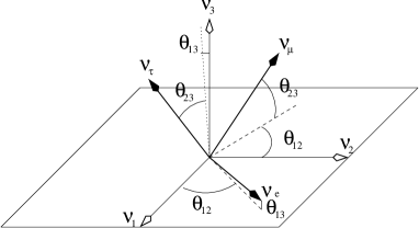
Figure 1: A graphical illustration of the MNS mixing angles. This figure ignores the phases so that the MNS matrix is constructed as a product of three Euler rotations $U_{MNS}=R_{23}R_{13}R_{12}$. The atmospheric angle is $\theta_{23}\approx\pi/4$, the CHOOZ angle is $\theta_{13}\buildrel<\over{{}_{\sim}}0.2$, and the solar angle is $\theta_{12}\approx\pi/6$.

There are basically two patterns of neutrino mass squared orderings consistent with the atmospheric and solar data as shown in Fig.2.

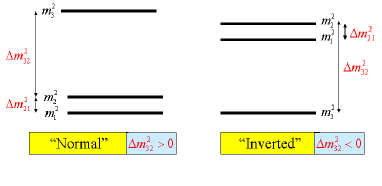
Figure 2: Alternative neutrino mass patterns that are consistent with neutrino oscillation explanations of the atmospheric and solar data. The absolute scale of neutrino masses is not fixed by oscillation data and the lightest neutrino mass may vary from 0.0-0.6 eV.

It is clear that neutrino oscillations, which only depend on $\Delta m_{ij}^{2}\equiv m_{i}^{2}-m_{j}^{2}$, gives no information about the absolute value of the neutrino mass squared eigenvalues $m_{i}^{2}$ in Fig2. Recent results from the 2df galaxy redshift survey indicate that $\sum m_{i}<1.8{\rm eV}(95\%C.L.)$ under certain mild assumptions [13, 14]. Combined with the solar and atmospheric oscillation data this brackets the heaviest neutrino mass to be in the approximate range 0.04-0.6 eV. The fact that the mass of the heaviest neutrino is known to within an order of magnitude represents remarkable progress in neutrino physics over recent years.

3 CONSTRUCTING THE MNS MATRIX

From a model building perspective the neutrino and charged lepton masses are given by the eigenvalues of a complex charged lepton mass matrix $m^{E}_{LR}$ and a complex symmetric neutrino Majorana matrix $m_{LL}$, obtained by diagonalising these mass matrices,

$$V^{E_{L}}m^{E}_{LR}{V^{E_{R}}}^{\dagger}=\left(\begin{array}[]{ccc}m_{e}&0&0\\ 0&m_{\mu}&0\\ 0&0&m_{\tau}\end{array}\right)$$ (6)

$$V^{\nu_{L}}m_{LL}{V^{\nu_{L}}}^{T}=\left(\begin{array}[]{ccc}m_{1}&0&0\\ 0&m_{2}&0\\ 0&0&m_{3}\end{array}\right)$$ (7)

where $V^{E_{L}}$, $V^{E_{R}}$, $V^{\nu_{L}}$ are unitary tranformations on the left-handed charged lepton fields $E_{L}$, right-handed charged lepton fields $E_{R}$, and left-handed neutrino fields $\nu_{L}$ which put the mass matrices into diagonal form with real eigenvalues.

The MNS matrix is then constructed by

$$U_{MNS}=V^{E_{L}}{V^{\nu_{L}}}^{\dagger}$$ (8)

The MNS matrix is constructed in Eq.8 as a product of a unitary matrix from the charged lepton sector $V^{E_{L}}$ and a unitary matrix from the neutrino sector ${V^{\nu_{L}}}^{\dagger}$. Each of these unitary matrices may be parametrised by its own mixing angles and phases analagous to the MNS parameters. As shown in [15] the MNS matrix can be expanded in terms of neutrino and charged lepton mixing angles and phases to leading order in the charged lepton mixing angles which are assumed to be small,

$$s_{23}e^{-i\delta_{23}} \approx s_{23}^{\nu_{L}}e^{-i\delta_{23}^{\nu_{L}}}-\theta_{23}^{E_{L}}c_{23}^{\nu_{L}}e^{-i\delta_{23}^{E_{L}}}$$ (9)

$$\theta_{13}e^{-i\delta_{13}} \approx \theta_{13}^{\nu_{L}}e^{-i\delta_{13}^{\nu_{L}}}-\theta_{13}^{E_{L}}c_{23}^{\nu_{L}}e^{-i\delta_{13}^{E_{L}}}$$ (10)

$$+ \theta_{12}^{E_{L}}s_{23}^{\nu_{L}}e^{i(-\delta_{23}^{\nu_{L}}-\delta_{12}^{E_{L}})}$$

$$s_{12}e^{-i\delta_{12}} \approx s_{12}^{\nu_{L}}e^{-i\delta_{12}^{\nu_{L}}}+\theta_{23}^{E_{L}}s_{12}^{\nu_{L}}e^{-i\delta_{12}^{\nu_{L}}}$$ (11)

$$+ \theta_{13}^{E_{L}}c_{12}^{\nu_{L}}s_{23}^{\nu_{L}}e^{i(\delta_{23}^{\nu_{L}}-\delta_{13}^{E_{L}})}$$

$$- \theta_{12}^{E_{L}}c_{23}^{\nu_{L}}c_{12}^{\nu_{L}}e^{-i\delta_{12}^{E_{L}}}$$

Clearly $\theta_{13}$ receives important contributions not just from $\theta_{13}^{\nu_{L}}$, but also from the charged lepton angles $\theta_{12}^{E_{L}}$, and $\theta_{13}^{E_{L}}$. In models where $\theta_{13}^{\nu_{L}}$ is extremely small, $\theta_{13}$ may originate almost entirely from the charged lepton sector. Charged lepton contributions could also be important in models where $\theta_{12}^{\nu_{L}}=\pi/4$, since charged lepton mixing angles may allow consistency with the LMA MSW solution. Such effects are important for the inverted hierarchy model [16, 15].

4 NEUTRINO MAJORANA MASS MATRICES

For many (but not all) purposes it is convenient to forget about the division between charged lepton and neutrino mixing angles and work in a basis where the charged lepton mass matrix is diagonal. Then the MNS angles and phases simply correspond to the neutrino ones. In this special basis the mass matrix is given from Eq.7 and Eq.8 as

$$m_{LL}=U_{MNS}\left(\begin{array}[]{ccc}m_{1}&0&0\\ 0&m_{2}&0\\ 0&0&m_{3}\end{array}\right)U_{MNS}^{T}$$ (12)

For a given assumed form of $U_{MNS}$ and set of neutrino masses $m_{i}$ one may use Eq.12 to “derive” the form of the neutrino mass matrix $m_{LL}$, and this results in the candidate mass matrices in Table 1 [17].

In Table 1 the mass matrices are classified into two types:

Type I - small neutrinoless double beta decay

Type II - large neutrinoless double beta decay

They are also classified into the limiting cases consistent with the mass squared orderings in Fig.2:

A - Normal hierarchy $m_{1}^{2},m_{2}^{2}\ll m_{3}^{2}$

B - Inverted hierarchy $m_{1}^{2}\approx m_{2}^{2}\gg m_{3}^{2}$

C - Approximate degeneracy $m_{1}^{2}\approx m_{2}^{2}\approx m_{3}^{2}$

Thus according to our classification there is only one neutrino mass matrix consistent with the normal neutrino mass hierarchy which we call Type IA, corresponding to the leading order neutrino masses of the form $m_{i}=(0,0,m)$. For the inverted hierarchy there are two cases, Type IB corresponding to $m_{i}=(m,-m,0)$ or Type IIB corresponding to $m_{i}=(m,m,0)$. For the approximate degeneracy cases there are three cases, Type IC correponding to $m_{i}=(m,-m,m)$ and two examples of Type IIC corresponding to either $m_{i}=(m,m,m)$ or $m_{i}=(m,m,-m)$.

At present experiment allows any of the matrices in Table 1. In future it will be possible to uniquely specify the neutrino matrix in the following way:

1. Neutrinoless double beta effectively measures the 11 element of the mass matrix $m_{LL}$ corresponding to

$$\beta\beta_{0\nu}\equiv\sum_{i}U_{ei}^{2}m_{i}$$ (13)

and is clearly capable of resolving Type I from Type II cases according to the bounds given in Table 1 [18]. There has been a recent claim of a signal in neutrinoless double beta decay correponding to $\beta\beta_{0\nu}=0.11-0.56$ eV at 95% C.L. [19]. However this claim has been criticised by two groups [20], [21] and in turn this criticism has been refuted [22]. Since the Heidelberg-Moscow experiment has almost reached its full sensitivity, we may have to wait for a next generation experiment such as GENIUS [23] which is capable of pushing down the sensitivity to 0.01 eV to resolve this question.

2. A neutrino factory will measure the sign of $\Delta m_{32}^{2}$ and resolve A from B.

3. Tritium beta decay experiments are sensitive to C since they measure the “electron neutrino mass” defined by

$$|m_{\nu_{e}}|\equiv\sum_{i}|U_{ei}|^{2}|m_{i}|.$$ (14)

For example the KATRIN [24] experiment has a proposed sensitivity of 0.35 eV. As already mentioned the galaxy power spectrum combined with solar and atmospheric oscillation data already limits the degenerate neutrino mass to be less than about 0.6 eV, and this limit is also expected to improve in the future. Also it is worth mentioning that in future it may be possible to measure neutrino masses from gamma ray bursts using time of flight techniques in principle down to 0.001 eV [25].

Type IIB and C involve small fractional mass splittings $|\Delta m_{ij}^{2}|\ll m^{2}$ which are unstable under radiative corrections [26], and even the most natural Type IC case is difficult to implement [27],[28]. Types IA and IB seem to be the most natural and later we shall focus on the normal hierarchy Type IA,

$$m_{LL}\sim\left(\begin{array}[]{ccc}0&0&0\\ 0&1&1\\ 0&1&1\\ \end{array}\right)\frac{m}{2}$$ (15)

However even Type IA models appear to have some remaining naturalness problem since $m_{3}\sim\sqrt{|\Delta m_{32}^{2}|}\sim 5.10^{-2}$ eV and $m_{2}\sim\sqrt{|\Delta m_{21}^{2}|}\sim 7.10^{-3}$ eV, compared to the natural expectation $m_{2}\sim m_{3}$. The question may be phrased in technical terms as one of understanding why the sub-determinant of the mass matrix in Eq.15 is small:

$$det\left(\begin{array}[]{cc}m_{22}&m_{23}\\ m_{23}&m_{33}\\ \end{array}\right)\ll m^{2}.$$ (16)

5 THE SEE-SAW MASS MECHANISM

Before discussing the see-saw mechanism it is worth first reviewing the different types of neutrino mass that are possible. So far we have been assuming that neutrino masses are Majorana masses of the form

$$m_{LL}\overline{\nu_{L}}\nu_{L}^{c}$$ (17)

where $\nu_{L}$ is a left-handed neutrino field and $\nu_{L}^{c}$ is the CP conjugate of a left-handed neutrino field, in other words a right-handed antineutrino field. Such Majorana masses are possible to qsince both the neutrino and the antineutrino are electrically neutral and so Majorana masses are not forbidden by electric charge conservation. For this reason a Majorana mass for the electron would be strictly forbidden. Majorana neutrino masses “only” violate lepton number conservation. If we introduce right-handed neutrino fields then there are two sorts of additional neutrino mass terms that are possible. There are additional Majorana masses of the form

$$M_{RR}\overline{\nu_{R}}\nu_{R}^{c}$$ (18)

where $\nu_{R}$ is a right-handed neutrino field and $\nu_{R}^{c}$ is the CP conjugate of a right-handed neutrino field, in other words a left-handed antineutrino field. In addition there are Dirac masses of the form

$$m_{LR}\overline{\nu_{L}}\nu_{R}.$$ (19)

Such Dirac mass terms conserve lepton number, and are not forbidden by electric charge conservation even for the charged leptons and quarks.

In the Standard Model Dirac mass terms for charged leptons and quarks are generated from Yukawa couplings to a Higgs doublet whose vacuum expectation value gives the Dirac mass term. Neutrino masses are zero in the Standard Model because right-handed neutrinos are not present, and also because the Majorana mass terms in Eq.17 require Higgs triplets in order to be generated at the renormalisable level (although non-renormalisable operators can be written down [5]). Higgs triplets are phenomenologically disfavoured so the simplest way to generate neutrino masses from a renormalisable theory is to introduce right-handed neutrinos. Once this is done then the types of neutrino mass discussed in Eqs.18,19 (but not Eq.17 since we have not introduced Higgs triplets) are permitted, and we have the mass matrix

$$\left(\begin{array}[]{cc}\overline{\nu_{L}}&\overline{\nu^{c}_{R}}\end{array}\\ \right)\left(\begin{array}[]{cc}0&m_{LR}\\ m_{LR}^{T}&M_{RR}\\ \end{array}\right)\left(\begin{array}[]{c}\nu_{L}^{c}\\ \nu_{R}\end{array}\\ \right)$$ (20)

Since the right-handed neutrinos are electroweak singlets the Majorana masses of the right-handed neutrinos $M_{RR}$ may be orders of magnitude larger than the electroweak scale. In the approximation that $M_{RR}\gg m_{LR}$ the matrix in Eq.20 may be diagonalised to yield effective Majorana masses of the type in Eq.17,

$$m_{LL}=m_{LR}M_{RR}^{-1}m_{LR}^{T}$$ (21)

This is the see-saw mechanism [29, 30]. It not only generates Majorana mass terms of the type $m_{LL}$, but also naturally makes them smaller than the Dirac mass terms by a factor of $m_{LR}/M_{RR}\ll 1$. One can think of the heavy right-handed neutrinos as being integrated out to give non-renormalisable Majorana operators suppressed by the heavy mass scale $M_{RR}$.

In a realistic model with three left-handed neutrinos and three right-handed neutrinos the Dirac masses $m_{LR}$ are a $3\times 3$ (complex) matrix and the heavy Majorana masses $M_{RR}$ form a separate $3\times 3$ (complex symmetric) matrix. The light effective Majorana masses $m_{LL}$ are also a $3\times 3$ (complex symmetric) matrix and continue to be given from Eq.21 which is now interpreted as a matrix product. From a model building perspective the fundamental parameters which must be input into the see-saw mechanism are the Dirac mass matrix $m_{LR}$ and the heavy right-handed neutrino Majorana mass matrix $M_{RR}$. The light effective left-handed Majorana mass matrix $m_{LL}$ arises as an output according to the see-saw formula in Eq.21. The goal of see-saw model building is therefore to choose input see-saw matrices $m_{LR}$ and $M_{RR}$ that will give rise to one of the successful matrices $m_{LL}$ in Table 1.

6 SINGLE RIGHT HANDED NEUTRINO DOMINANCE

We now show how the input see-saw matrices can be simply chosen to give the Type IA matrix in Eq.15, with the property of a naturally small sub-determinant in Eq.16 using a mechanism first suggested in [31]. The idea was developed in [32] where it was called single right-handed neutrino dominance (SRHND) . SRHND was first successfully applied to the LMA MSW solution in [33].

The SRHND mechanism is most simply described assuming three right-handed neutrinos in the basis where the right-handed neutrino mass matrix is diagonal although it can also be developed in other bases [32, 33]. In this basis we write the input see-saw matrices as

$$M_{RR}=\left(\begin{array}[]{ccc}X^{\prime}&0&0\\ 0&X&0\\ 0&0&Y\end{array}\right)$$ (22)

$$m_{LR}=\left(\begin{array}[]{ccc}a^{\prime}&a&d\\ b^{\prime}&b&e\\ c^{\prime}&c&f\end{array}\right)$$ (23)

In [31] it was suggested that one of the right-handed neutrinos may dominante the contribution to $m_{LL}$ if it is lighter than the other right-handed neutrinos. The dominance condition was subsequently generalised to include other cases where the right-handed neutrino may be heavier than the other right-handed neutrinos but dominates due to its larger Dirac mass couplings [32]. In any case the dominant neutrino may be taken to be the third one without loss of generality. Assuming SRHND then Eqs.21, 22, 23 give

$$m_{LL}\approx\left(\begin{array}[]{ccc}\frac{d^{2}}{Y}&\frac{de}{Y}&\frac{df}{Y}\\ .&\frac{e^{2}}{Y}&\frac{ef}{Y}\\ .&.&\frac{f^{2}}{Y}\end{array}\right)$$ (24)

If the Dirac mass couplings satisfy the condition $d\ll e\approx f$ [31] then the matrix in Eq.24 resembles the Type IA matrix in Eq.15, and furthermore has a naturally small sub-determinant as in Eq.16. The neutrino mass spectrum consists of one neutrino with mass $m_{3}\approx(e^{2}+f^{2})/Y$ and two approximately massless neutrinos [31]. The atmospheric angle is $\tan\theta_{23}\approx e/f$ [31]. It was pointed out that small perturbations from the sub-dominant right-handed neutrinos can then lead to a small solar neutrino mass splitting [31].

It was subsequently shown how to account for the LMA MSW solution with a large solar angle [33] by careful consideration of the sub-dominant contributions. One of the examples considered in [33] is when the right-handed neutrinos dominate sequentially,

$$\frac{|e^{2}|,|f^{2}|,|ef|}{Y}\gg\frac{|xy|}{X}\gg\frac{|x^{\prime}y^{\prime}|}{X^{\prime}}$$ (25)

where $x,y\in a,b,c$ and $x^{\prime},y^{\prime}\in a^{\prime},b^{\prime},c^{\prime}$. Assuming SRHND with sequential sub-dominance as in Eq.25, then Eqs.21, 22, 23 give

$$m_{LL}\approx\left(\begin{array}[]{ccc}\frac{a^{2}}{X}+\frac{d^{2}}{Y}&\frac{ab}{X}+\frac{de}{Y}&\frac{ac}{X}+\frac{df}{Y}\\ .&\frac{b^{2}}{X}+\frac{e^{2}}{Y}&\frac{bc}{X}+\frac{ef}{Y}\\ .&.&\frac{c^{2}}{X}+\frac{f^{2}}{Y}\end{array}\right)$$ (26)

where the contribution from the first right-handed neutrino may be neglected according to Eq.25. This was show to lead to a full neutrino mass hierarchy

$$m_{1}^{2}\ll m_{2}^{2}\ll m_{3}^{2}$$ (27)

and, ignoring phases, the solar angle only depends on the sub-dominant couplings and is given by $\tan\theta_{12}\approx a/(c_{23}b-s_{23}c)$ [33]. The simple requirement for large solar angle is then $a\sim b-c$ [33]. Including phases the solar angle is given by the analagous result [15]

$$\tan\theta_{12}\approx\frac{|a|}{c_{23}|b|\cos\phi_{b}^{\prime}-s_{23}|c|\cos\phi_{c}^{\prime}}$$ (28)

where the phases $\phi_{b}^{\prime},\phi_{c}^{\prime}$ are defined in [15]. A related phase analysis which pointed out the importance of phases for determining the solar angle was given in [34]. One also obtains the interesting bound on the angle $\theta_{13}$, [15, 34, 35, 20]

$$\theta_{13}\buildrel>\over{{}_{\sim}}\frac{m_{2}}{m_{3}}\sim 0.1$$ (29)

which implies that $\theta_{13}$ should be just below the CHOOZ limit [36], and there is therfore a good chance that this angle could be observed at MINOS or CNGS.

7 SUSY, GUTs AND FAMILY SYMMETRIES

One of the exciting things about the discovery of neutrino masses and mixing angles is that this provides additional information about the flavour problem - the problem of understanding the origin of three families of quarks and leptons and their masses and mixing angles (Fig.3). Solutions to the flavour problem typically involve introducing a Family symmetry $G_{{\rm Family}}$, which unifies the three families as shown in Fig.3.

In the framework of the see-saw mechanism, new physics beyond the standard model is required to violate lepton number and generate right-handed neutrino masses which are typically around the GUT scale. This is also exciting since it implies that the origin of neutrino masses is also related to some GUT symmetry group $G_{{\rm GUT}}$, which unifies the fermions within each family as shown in Fig.3.

It is well known that such large mass scales can only be stabilised by assuming a TeV scale N=1 SUSY which cancels the quadratic divergences of the Higgs mass, and in turn SUSY enables the gauge couplings to meet at the GUT scale to give a self-consistent unification picture.

Putting these ideas to together we are suggestively led to a framework of new physics beyond the standard model based on N=1 SUSY with commuting GUT and Family symmetry groups,

$$G_{{\rm GUT}}\times G_{{\rm Family}}$$ (30)

There are many possible candidate GUT and Family symmetry groups some of which are listed in Table 2. Unfortunately the model dependence does not end there, since the details of the symmetry breaking vacuum plays a crucial role in specifying the model and determining the masses and mixing angles, resulting in many models [8, 37].

Another complication is that the masses and mixing angles determined in some high energy theory must be run down to low energies using the renormalisation group equations (RGEs) [38, 39]. Large radiative corrections are seen [40] when the see-saw parameters are tuned, since the spectrum is sensitive to small changes in the parameters. In natural models based on SRHND the parameters are not tuned, since the hierarchy and large atmospheric and solar angles arise naturally as discussed in the previous section. Therefore in SRHND models the radiative corrections to neutrino masses and mixing angles are only expected to be a few per cent, and this has been verified numerically [41].

In the next section we give two examples of models with the symmetry structure of Eq.30 which incorporate SRHND.

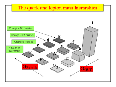
Figure 3: The fermion masses are here represented by a lego plot. We have multiplied the masses of the bottom, charm and tau by $10$, the strange and muon by $10^{2}$, the up and down by $10^{3}$, the electron by $10^{4}$ to make the lego blocks visible. It is natural to assume a normal neutrino hierarchy. We have multiplied the third neutrino mass by $10^{11}$ and the second neutrino mass by $10^{12}$ to make the lego blocks visible. This underlines how incredibly light the neutrinos are. The symmetry groups $G_{{\rm GUT}}$ and $G_{{\rm Family}}$ act in the directions indicated.

8 TWO EXAMPLES

8.1 $SU(5)_{{\rm GUT}}\times U(1)_{{\rm Family}}$

A simple example assigns $U(1)_{{\rm Family}}$ charges to $SU(5)_{{\rm GUT}}$ multiplets labelled by a family index, $\overline{5_{i}}=(L_{i},D^{c}_{i})$, ${10_{i}}=(Q,U^{c}_{i},E^{c}_{i})$, $1_{i}=N^{c}_{i}$, as follows [42]:

$$\overline{5_{i}}=(3,0,0),\ \ {10_{i}}=(3,2,0),\ \ 1_{i}=(1,-1,0)$$ (31)

Note that three right-handed neutrinos have been added by hand. This results in the neutrino see-saw matrices [42]

$$m_{LR}\sim\left(\begin{array}[]{ccc}\lambda^{4}&\lambda^{2}&\lambda^{3}\\ \lambda&\lambda&1\\ \lambda&\lambda&1\end{array}\right)$$ (32)

$$M_{RR}\sim\left(\begin{array}[]{ccc}\lambda^{2}&1&\lambda\\ 1&\lambda^{2}&\lambda\\ \lambda&\lambda&1\end{array}\right)$$ (33)

where $\lambda\approx 0.22$ is assumed to be of order the Cabibbo angle. Although the three right-handed neutrinos are roughly degenerate, this model has SRHND since the third right-handed neutrino dominates due to its larger Dirac mass couplings. A large atmospheric angle is given from the large entry in the 23 position of the “lop-sided” neutrino mass matrix $\tan\theta_{23}\approx e/f\sim 1$. The solar angle is $\tan\theta_{12}\sim a/(b-c)\sim\lambda$ which may be interpreted as either LMA or SMA MSW. The quark mass matrices are given by

$$m_{LR}^{D}\sim\left(\begin{array}[]{ccc}\lambda^{6}&\lambda^{3}&\lambda^{3}\\ \lambda^{5}&\lambda^{2}&\lambda^{2}\\ \lambda^{3}&1&1\end{array}\right)$$ (34)

$$m_{LR}^{U}\sim\left(\begin{array}[]{ccc}\lambda^{6}&\lambda^{5}&\lambda^{3}\\ \lambda^{5}&\lambda^{4}&\lambda^{2}\\ \lambda^{3}&\lambda^{2}&1\end{array}\right)$$ (35)

The down mass matrix only has large unphysical right-handed mixing with small physical left-handed quark mixing angles. The mass and mixing relations are:

$$V_{us}\sim\lambda,\ \ V_{ub}\sim\lambda^{3},\ \ V_{cb}\sim\lambda^{2}$$ (36)

$$m_{u}:m_{c}:m_{t}=\lambda^{6}:\lambda^{4}:1$$ (37)

$$m_{d}:m_{s}:m_{b}=\lambda^{6}:\lambda^{2}:1$$ (38)

8.2 $SO(10)_{{\rm GUT}}\times SU(3)_{{\rm Family}}$

In this model [43], the three families are unified as triplets under $SU(3)_{{\rm Family}}$, and $16^{\prime}s$ under $SO(10)_{{\rm GUT}}$. Further symmetries are assumed to ensure that the vacuum alignment leads to a universal form of Dirac mass matrices for the neutrinos, charged leptons and quarks [43],

$$m_{LR}\sim\left(\begin{array}[]{ccc}\epsilon^{8}&\epsilon^{3}&\epsilon^{3}\\ -\epsilon^{3}&\epsilon^{2}&\epsilon^{2}\\ -\epsilon^{3}&\epsilon^{2}&1\end{array}\right)$$ (39)

where $\epsilon\approx 0.05$ and the expansion parameter for the down quarks and charged leptons is assumed to be larger $\overline{\epsilon}\approx 0.15$.

The neutrino see-saw matrices are [43],

$$m_{LR}\sim\left(\begin{array}[]{ccc}\epsilon^{8}&\lambda_{\nu}\epsilon^{3}&\lambda_{\nu}\epsilon^{3}\\ -\lambda_{\nu}\epsilon^{3}&a_{\nu}\epsilon^{2}&a_{\nu}\epsilon^{2}+\lambda^{\prime}_{\nu}\epsilon^{3}\\ -\lambda_{\nu}\epsilon^{3}&a_{\nu}\epsilon^{2}+\lambda^{\prime}_{\nu}\epsilon^{3}&1\end{array}\right)$$ (40)

where $\lambda_{\nu},\lambda^{\prime}_{\nu},a_{\nu}$ are order one parameters.

$$M_{RR}\sim\left(\begin{array}[]{ccc}\epsilon_{\nu}^{4}&0&\epsilon_{\nu}^{2}\\ 0&\epsilon_{\nu}^{3}&\epsilon_{\nu}^{3}\\ \epsilon_{\nu}^{2}&\epsilon_{\nu}^{3}&1\end{array}\right)$$ (41)

In this model the first right-handed neutrino dominates because the expansion parameter $\epsilon_{\nu}$ is very small so it is very light, leading to SRHND with sequential sub-dominance as in Eq.25. The strong hierarchy tends to predict the LOW solution, although LMA MSW is also possible [43]. The results in section 6 apply after re-ordering the columns to make the first right-handed neutrino the dominant one,

$$m_{LR}=\left(\begin{array}[]{ccc}d&a&a^{\prime}\\ e&b&b^{\prime}\\ f&c&c^{\prime}\end{array}\right)$$ (42)

The atmospheric angle is given from section 6 by $\tan\theta_{23}\approx e/f$ where the $SU(3)_{{\rm Family}}$ symmetry ensures accurate equality $e=f=-\lambda_{\nu}\epsilon^{3}$. The solar angle is given from section 6 by $\tan\theta_{12}\sim a/(b-c)\sim-\lambda_{\nu}/\lambda^{\prime}_{\nu}\sim 1$ where the $SU(3)_{{\rm Family}}$ symmetry leads to a cancellation of the leading order terms and a large solar angle. The quark mass matrices are

$$m^{U}_{LR}\sim\left(\begin{array}[]{ccc}\epsilon^{8}&\lambda_{U}\epsilon^{3}&\lambda_{U}\epsilon^{3}\\ -\lambda_{U}\epsilon^{3}&\epsilon^{2}&\epsilon^{2}\\ -\lambda_{U}\epsilon^{3}&\epsilon^{2}&1\end{array}\right)$$ (43)

$$m^{D}_{LR}\sim\left(\begin{array}[]{ccc}\overline{\epsilon}^{8}&\lambda_{D}\overline{\epsilon}^{3}&\lambda_{D}\overline{\epsilon}^{3}\\ -\lambda_{D}\overline{\epsilon}^{3}&\overline{\epsilon}^{2}&\overline{\epsilon}^{2}\\ -\lambda_{D}\overline{\epsilon}^{3}&\overline{\epsilon}^{2}&1\end{array}\right)$$ (44)

where $\lambda_{U},\lambda_{D}$ are order one parameters, which provides a very good description of the quark masses and mixing angles [43]. The fact that the first right-handed neutrino dominates is the key which allows large neutrino mixing angles to arise from a universal form of mass matrix with only small off-diagonal entries.

9 CONCLUSIONS

I have reviewed promising approaches to neutrino mass models, focussing on three neutrino patterns of neutrino masses and mixing angles, and the corresponding Majorana mass matrices classified in Table 1. I also reviewed the see-saw mechanism which at the present time looks like the most elegant explanation of small neutrino masses. If the see-saw mechanism for understanding the neutrino spectrum looks good, with SRHND it looks even better. With SRHND the neutrino hierarchy appears very naturally, and large atmospheric and solar angles are understood in terms of simple analytic relations between Dirac mass elements. I described an attractive theoretical framework for understanding quark and lepton (including neutrino) masses and mixing angles based on SUSY, GUTs and Family symmetry. Two examples of such models were discussed which implement the see-saw mechanism using SRHND, where the relations responsible for large atmospheric and solar angles could be understood in terms of symmetries.

Table 1: Leading order low energy neutrino Majorana mass matrices $m_{LL}$ consistent with large atmospheric and solar mixing angles, classified according to the rate of neutrinoless double beta decay and the pattern of neutrino masses.

	Type I	Type II
	Small $\beta\beta_{0\nu}$	Large $\beta\beta_{0\nu}$
A	$\beta\beta_{0\nu}\buildrel<\over{{}_{\sim}}0.0082$ eV
Normal hierarchy
$m_{1}^{2},m_{2}^{2}\ll m_{3}^{2}$	$\left(\begin{array}[]{ccc}0&0&0\\ 0&1&1\\ 0&1&1\\ \end{array}\right)\frac{m}{2}$	–
B	$\beta\beta_{0\nu}\buildrel<\over{{}_{\sim}}0.0082$ eV	$\beta\beta_{0\nu}\buildrel>\over{{}_{\sim}}0.0085$ eV
Inverted hierarchy
$m_{1}^{2}\approx m_{2}^{2}\gg m_{3}^{2}$	$\left(\begin{array}[]{ccc}0&1&1\\ 1&0&0\\ 1&0&0\\ \end{array}\right)\frac{m}{\sqrt{2}}$	$\left(\begin{array}[]{ccc}1&0&0\\ 0&\frac{1}{2}&\frac{1}{2}\\ 0&\frac{1}{2}&\frac{1}{2}\\ \end{array}\right)m$
C		$\beta\beta_{0\nu}\buildrel>\over{{}_{\sim}}0.035$ eV
Approximate degeneracy		diag(1,1,1)m
$m_{1}^{2}\approx m_{2}^{2}\approx m_{3}^{2}$	$\left(\begin{array}[]{ccc}0&\frac{1}{\sqrt{2}}&\frac{1}{\sqrt{2}}\\ \frac{1}{\sqrt{2}}&\frac{1}{2}&\frac{1}{2}\\ \frac{1}{\sqrt{2}}&\frac{1}{2}&\frac{1}{2}\\ \end{array}\right)m$	$\left(\begin{array}[]{ccc}1&0&0\\ 0&0&1\\ 0&1&0\\ \end{array}\right)m$

Table 2: Some candidate GUT and Family symmetry groups.

$G_{{\rm GUT}}$	$G_{{\rm Family}}$
$E_{6}$	$SU(3)$
$SO(10)$	$SU(2)$
$SU(5)$	$U(1)$
$SU(5)\times U(1)$	$Z_{N}$
$SU(3)^{3}$	$O(3)\times O(3)$
$SU(4)\times SU(2)\times SU(2)$	$SO(3)$
$SU(3)\times SU(2)\times SU(2)\times U(1)$	$S(3)\times S(3)$
$SU(3)\times SU(2)\times U(1)\times U(1)$	$S(3)$
$SU(3)\times SU(2)\times U(1)$	Nothing

References

- [1] A. Hallin, these proceedings.
- [2] M. Smy, these proceedings.
- [3] A, Smirnov, these proceedings.
- [4] E. Lisi, these proceedings.
- [5] J. W. F. Valle, these proceedings.
- [6] M.Shiozawa, these proceedings.
- [7] M. Apollonio et al. [CHOOZ Collaboration], Phys. Lett. B 466 (1999) 415 [arXiv:hep-ex/9907037]. [8]
- [8] For a recent review see: G. Altarelli and F. Feruglio, arXiv:hep-ph/0206077.
- [9] G. Drexlin, these proceedings.
- [10] R. Tayloe, these proceedings.
- [11] Z. Maki, M. Nakagawa and S. Sakata, Prog. Theor. Phys. 28 (1962) 870.
- [12] B. W. Lee, S. Pakvasa, R. E. Shrock and H. Sugawara, Phys. Rev. Lett. 38 (1977) 937 [Erratum-ibid. 38 (1977) 1230].
- [13] O. Elgaroy et al., galaxy redshift survey,” arXiv:astro-ph/0204152.
- [14] S. Hannestad, these proceedings.
- [15] S. F. King, arXiv:hep-ph/0204360.
- [16] S. F. King and N. N. Singh, Nucl. Phys. B 596 (2001) 81 [arXiv:hep-ph/0007243].
- [17] R. Barbieri, L. J. Hall, D. R. Smith, A. Strumia and N. Weiner, JHEP 9812 (1998) 017 [arXiv:hep-ph/9807235].
- [18] S. Pascoli and S. T. Petcov, arXiv:hep-ph/0205022.
- [19] H. V. Klapdor-Kleingrothaus, A. Dietz, H. L. Harney and I. V. Krivosheina, Mod. Phys. Lett. A 16 (2001) 2409 [arXiv:hep-ph/0201231].
- [20] F. Feruglio, A. Strumia and F. Vissani, arXiv:hep-ph/0201291.
- [21] C. E. Aalseth et al., arXiv:hep-ex/0202018.
- [22] H. V. Klapdor-Kleingrothaus, arXiv:hep-ph/0205228.
- [23] O.Cremonesi, these proceedings.
- [24] Ch.Weinheimer, these proceedings.
- [25] S. Choubey and S. F. King, arXiv:hep-ph/0207260.
- [26] J. R. Ellis and S. Lola, Phys. Lett. B 458 (1999) 310 [arXiv:hep-ph/9904279].
- [27] R. Barbieri, L. J. Hall, G. L. Kane and G. G. Ross, arXiv:hep-ph/9901228.
- [28] P. H. Chankowski, A. Ioannisian, S. Pokorski and J. W. Valle, Phys. Rev. Lett. 86 (2001) 3488 [arXiv:hep-ph/0011150].
- [29] M. Gell-Mann, P. Ramond and R. Slansky in Sanibel Talk, CALT-68-709, Feb 1979, and in Supergravity (North Holland, Amsterdam 1979); T. Yanagida in Proc. of the Workshop on Unified Theory and Baryon Number of the Universe, KEK, Japan, 1979.
- [30] R. N. Mohapatra and G. Senjanovic, Phys. Rev. Lett. 44 (1980) 912; J. Schechter and J. W. Valle, Phys. Rev. D 25 (1982) 774.
- [31] S. F. King, Phys. Lett. B 439 (1998) 350 [arXiv:hep-ph/9806440].
- [32] S. F. King, Nucl. Phys. B 562 (1999) 57 [arXiv:hep-ph/9904210].
- [33] S. F. King, Nucl. Phys. B 576 (2000) 85 [arXiv:hep-ph/9912492].
- [34] S. Lavignac, I. Masina and C. A. Savoy, arXiv:hep-ph/0202086.
- [35] E. K. Akhmedov, G. C. Branco and M. N. Rebelo, Phys. Rev. Lett. 84 (2000) 3535 [arXiv:hep-ph/9912205].
- [36] F. Vissani, JHEP 9811 (1998) 025 [arXiv:hep-ph/9810435].
- [37] C. H. Albright and S. M. Barr, Phys. Rev. D 58, 013002 (1998); N. Irges, S. Lavignac and P. Ramond, Phys. Rev. D 58, 035003 (1998); Z. Berezhiani and A. Rossi, JHEP 9903, 002 (1999); R. Barbieri, P. Creminelli and A. Romanino, Nucl. Phys. B559 (1999) 17, hep-ph/9903460; T. Ohlsson and G. Seidl, arXiv:hep-ph/0206087; H. Fritzsch and Z. z. Xing, Prog. Part. Nucl. Phys. 45 (2000) 1 [arXiv:hep-ph/9912358]; W. Grimus and L. Lavoura, JHEP 0107 (2001) 045 [arXiv:hep-ph/0105212]; E. K. Akhmedov, G. C. Branco, F. R. Joaquim and J. I. Silva-Marcos, Phys. Lett. B 498 (2001) 237 [arXiv:hep-ph/0008010]; R. Kuchimanchi and R. N. Mohapatra, arXiv:hep-ph/0207110; J. C. Pati, arXiv:hep-ph/0204240; S. F. King and M. Oliveira, Phys. Rev. D 63 (2001) 095004 [arXiv:hep-ph/0009287]; M. Hirsch and S. F. King, Phys. Rev. D 64 (2001) 113005 [arXiv:hep-ph/0107014]; T. Blazek and S. F. King, Phys. Lett. B 518 (2001) 109 [arXiv:hep-ph/0105005].
- [38] K. S. Babu, C. N. Leung and J. Pantaleone, Phys. Lett. B 319 (1993) 191 [arXiv:hep-ph/9309223].
- [39] S. Antusch and M. Ratz, arXiv:hep-ph/0203027; S. Antusch, M. Drees, J. Kersten, M. Lindner and M. Ratz, Phys. Lett. B 519 (2001) 238 [arXiv:hep-ph/0108005]; S. Antusch, M. Drees, J. Kersten, M. Lindner and M. Ratz, Phys. Lett. B 525 (2002) 130 [arXiv:hep-ph/0110366].
- [40] J. R. Ellis, G. K. Leontaris, S. Lola and D. V. Nanopoulos, Eur. Phys. J. C 9 (1999) 389 [arXiv:hep-ph/9808251].
- [41] S. F. King and N. N. Singh, Nucl. Phys. B 591 (2000) 3 [arXiv:hep-ph/0006229].
- [42] G. Altarelli and F. Feruglio, Phys. Lett. B 451 (1999) 388 [arXiv:hep-ph/9812475].
- [43] S. F. King and G. G. Ross, Phys. Lett. B 520 (2001) 243 [arXiv:hep-ph/0108112]; G. G. Ross and L.Velasco-Sevila, arXiv:hep-ph/0208218.