Triplet Higgs boson at hadron colliders

Abstract:

The novel feature of a Higgs-triplet representation is a nonzero tree-level coupling of $H^{+}W^{-}Z$, which is absent in all Higgs-doublet models. We study the associated production of a singly-charged Higgs boson of the Higgs-triplet representation with a $W$ or $Z$ boson at hadron colliders, followed by the $H^{+}\to W^{+}Z$ decay. We find that the $2\ell+4j$ final state gives an interesting level of signal with a negligible background, plus it allows a full mass reconstruction of the charged-Higgs boson. The cover range of the charged-Higgs mass is between 110 and 200 GeV.

1 Introduction

The Higgs boson is still at large under all present serious efforts in searching for it. The present lower limit on the standard model (SM) Higgs boson is 114.1 GeV at 95% C.L. from LEP Collaborations [1]. The limit on the light neutral-scalar Higgs boson of the minimal supersymmetric standard model (MSSM) is 91.0 GeV [2]. It starts to push into the region that is not so favored by the electroweak precision measurements [3]. Experimenters should also search for the Higgs-boson signals other than the usual SM or MSSM Higgs bosons. Models with more than one Higgs doublet often predict the existence of charged-Higgs bosons, which may be singly-, doubly, or even triply-charged. One particularly interesting channel to look for a charged-Higgs boson is via its coupling to $WZ$. The reason behind is that if there exists a tree-level coupling of $H^{+}W^{-}Z$, the Higgs boson must belong to a Higgs structure more complicated than just doublets (e.g., in MSSM with two Higgs doublets there is no tree-level $H^{+}W^{-}Z$ coupling.) A triplet representation is a typical example of this kind.

In extensions of the SM with Higgs doublets and singlets, the coupling $H^{+}W^{-}Z$ vanishes at tree level and can only be generated at one-loop level [4, 5]. The vanishing of the $H^{+}W^{-}Z$ coupling in the Lagrangian is due to the hypercharge ($Y$) and weak-isospin assignments of the Higgs representations introduced in the model. In addition, in multi-Higgs-doublet models, the resulting strength of the loop-induced $H^{+}W^{-}Z$ coupling turns out to be rather small, of the order of $10^{-2}$ relative to the SM vertex $HW^{+}W^{-}$. Therefore, a large $H^{+}W^{-}Z$ coupling is an indicator of triplet or higher Higgs representations beyond doublet models. Therefore, a search for the charged-Higgs boson in the $H^{+}W^{-}Z$ channel would be a test for new physics beyond Higgs-doublet models.

The potential of LEPII and the future TeV $e^{+}e^{-}$ colliders in differentiating the charged-Higgs bosons of a triplet from a doublet representation had been studied in Refs. [6, 7, 8]. Here we attempt to search for such a singly-charged Higgs boson of the triplet representation at hadron colliders, with emphasis on the Run II at the Tevatron. Note that the complex-triplet representations also predict a doubly-charged Higgs boson (i.e. $H^{++}$), which couples to a pair of same-charged leptons. Studies of this signature had been done in Ref. [9] for $H^{++}$ at hadron colliders, in Ref. [10] for $H^{--}$ production at $e^{-}e^{-}$ linear colliders, and in Ref. [11] for doubly-charged Higgs pair production at photon colliders.

The organization is as follows. In the next section, we briefly describe a viable model of Higgs-triplet representation. In Sec. III, we highlight some current bounds on this model. In Sec. IV, we calculate the associated production of the charged-Higgs boson with a $W$ or $Z$ boson, and discuss the possible signatures over the backgrounds. We conclude in Sec. V.

2 The Model

Here we consider the triplet-Higgs model by Galison [12], and by Georgi and Machacek [13]. They introduced more than one Higgs-triplet field into the model and imposed an $SU(2)$ custodial symmetry on the vacuum expectation values and hypercharges of the Higgs multiplets to ensure $\rho=1$ at tree level. Stability conditions of the $SU(2)$ custodial symmetry in the Higgs potential under higher-order quantum corrections were further analyzed by Chanowitz and Golden [14]. The model consists of a SM $Y=1$ complex doublet $\Phi$, plus one real $Y=0$ triplet and one complex $Y=2$ triplet. We follow closely the convention of Ref. [15]

$$\phi=\left(\begin{array}[]{cc}\phi^{0^{*}}&\phi^{+}\\ \phi^{-}&\phi^{0}\end{array}\right)\;,\qquad\Delta\ =\ \left(\begin{array}[]{ccc}\chi^{0}&\xi^{+}&\chi^{++}\\ \chi^{-}&\xi^{0}&\chi^{+}\\ \chi^{--}&\xi^{-}&\chi^{0\ast}\end{array}\right).$$ (1)

The tree-level gauge-boson masses are fixed by the kinetic energy terms of the Higgs bosons, which are

$${\cal L}=\frac{1}{2}\,{\rm Tr}\left[(D_{\mu}\phi)^{\dagger}(D^{\mu}\phi)\right]+\frac{1}{2}\,{\rm Tr}\left[(D_{\mu}\chi)^{\dagger}(D^{\mu}\chi)\right]\;,$$

where $D_{\mu}\phi$ and $D_{\mu}\chi$ are the covariant derivatives taking into account the SU(2) in $2\times 2$ and $3\times 3$ representations, respectively. In order to preserve $\rho=1$, a custodial SU(2)_R symmetry is imposed such that the Lagrangian is invariant under the global SU(2)${}_{L}\times$ SU(2)_R symmetry. In particular, the tree-level invariance of the gauge-boson mass terms under this custodial SU(2)_R symmetry is arranged by giving $\chi^{0}$ and $\xi^{0}$ the same vacuum expectation value (VEV). The VEVs for the fields are defined as

$$\langle\phi^{0}\rangle=\frac{v_{D}}{\sqrt{2}}\,,\qquad\langle\chi^{0}\rangle=\langle\xi^{0}\rangle=v_{T}\;.$$

It is also convenient to define

$$v^{2}=v_{D}^{2}+8v_{T}^{2}\;,\qquad\sin\theta_{H}=\frac{\sqrt{8}v_{T}}{\sqrt{v_{D}^{2}+8v^{2}_{T}}}\;,\qquad\cos\theta_{H}=\frac{v_{D}}{\sqrt{v_{D}^{2}+8v^{2}_{T}}}\;,$$ (2)

where $\theta_{H}$ is the doublet-triplet mixing angle.

By absorbing the Goldstone bosons the $W$ and $Z$ bosons acquire masses given by $m_{W}=gv/2$ and $m_{Z}=m_{W}/\cos^{2}\theta_{\rm w}$. The original number of degrees of freedom in the Higgs sector is 13 (1 complex doublet, 1 real triplet, and 1 complex triplet). Therefore, after 3 degrees of freedom become the longitudinal components of the gauge bosons, there are 10 physical states, which form one five-plet, one three-plet, and two singlets:

$$H_{5}=(H^{++}_{5},\,H^{+}_{5},\,H^{0}_{5},\,H^{-}_{5},\,H^{--}_{5})^{T}\;,\qquad H_{3}=(H^{+}_{3},\,H^{0}_{3},\,H^{-}_{3})^{T}\;,H_{1}^{0},\,H_{1}^{0^{\prime}}\;,$$ (3)

which are given in terms of the original fields as

$$H_{5}^{++} = \chi^{++}\,,\;\;H_{5}^{+}=\frac{1}{\sqrt{2}}(\chi^{+}-\xi^{+})\,,\;\;H_{5}^{0}=\frac{1}{\sqrt{6}}(2\xi^{0}-\sqrt{2}\chi^{0})\,,$$

$$H_{3}^{+} = \frac{\cos\theta_{H}}{\sqrt{2}}(\chi^{+}+\xi^{+})-\sin\theta_{H}\phi^{+}\;,\;\;H_{3}^{0}=i(\cos\theta_{H}\chi^{0i}+\sin\theta_{H}\phi^{0i})\;,$$

$$H^{0}_{1} = \phi^{0r}\,,\;\;H_{1}^{0^{\prime}}=\frac{1}{\sqrt{3}}(\sqrt{2}\chi^{0r}+\xi^{0})\;.$$ (4)

These Higgs fields can also mix. However, if the custodial SU(2) symmetry is preserved in the Higgs potential, the five-plet and three-plet will not mix with each other or with the singlets. The only possible mixing is between the two singlets. For simplicity we assume no further mixing of the above states and so they are the physical Higgs states.

Phenomenology is mainly determined by the Higgs couplings to fermions and gauge bosons. Recalling that the standard Yukawa coupling is via the doublet-Higgs fields to the fermion-antifermion pair, the coupling of a Higgs state to a fermion-antifermion pair is determined by its doublet component. Thus, the whole $H_{5}$ and $H_{1}^{0^{\prime}}$ have no fermion-antifermion couplings. The only fermionic coupling of $H_{5}$ is the $H_{5}^{++}\ell^{-}\ell^{-}$ coupling, which is not present in the SM. Other than that, only $H_{3}$ and $H_{1}^{0}$ have fermionic couplings. On the other hand, $H_{3}$ has no tree-level coupling to gauge bosons while all the others have. A novel feature is the existence of a nonzero tree-level coupling of $H_{5}^{+}$ to $W^{-}Z$, which is absent in all Higgs-doublet models. The observation of such a coupling necessarily signals a Higgs structure more complicated than doublets. This is the main motivation of the present work.

The corresponding vertex $H_{5}^{+}W^{-}Z$ is given by [15]

$${\cal L}_{int}\ =\ -g\frac{\sin\theta_{H}}{\cos\theta_{\rm w}}\,M_{W}H^{+}_{5}W^{-\mu}Z_{\mu}\ +\ h.c.,$$ (5)

where $g$ is the usual $SU(2)_{L}$ electroweak coupling constant, $\cos^{2}\theta_{\rm w}=1-\sin^{2}\theta_{\rm w}=M^{2}_{W}/M^{2}_{Z}$ at tree-level, and $\theta_{\rm w}$ is the Weinberg angle. Due to the electromagnetic gauge invariance, the coupling $H_{5}^{+}W^{-}\gamma$ is absent at tree level. As emphasized earlier, we are interested in a large $H_{5}^{+}W^{-}Z$ coupling that will unavoidably signify the triplet nature of the charged-Higgs boson $H_{5}^{+}$. However, this can only be possible experimentally if $\sin\theta_{H}\sim 1$ or equivalently $v_{T}\sim v_{D}$, which is considered to be a natural scenario. The partial width of $H^{+}_{5}\to W^{+}Z$ is given by

$$\Gamma(H^{+}_{5}\to W^{+}Z)=\frac{\alpha_{w}\sin^{2}\theta_{H}}{16}\;M_{H_{5}}\lambda^{1/2}\left(\frac{M^{2}_{H_{5}}}{M^{2}_{W}},\frac{1}{\cos^{2}\theta_{\rm w}},1\right)\,\Big{[}1+x_{W}^{2}+x_{Z}^{2}-2x_{W}-2x_{Z}+10x_{W}x_{Z}\Big{]}\;$$ (6)

with $\alpha_{w}=g^{2}/4\pi$, $\lambda(x,y,z)=(x-y-z)^{2}-4yz$, $x_{W}=M_{W}^{2}/M_{H_{5}}^{2}$, and $x_{Z}=M_{Z}^{2}/M_{H_{5}}^{2}$.

There are other triple vertices that will affect the decay of the $H_{5}^{+}$. They are $H_{5}^{+}H_{3}^{0}W^{-}$ and $H_{5}^{+}H_{3}^{-}Z$, the vertex factors of which are given by $-ig\cos\theta_{H}(p-p^{\prime})^{\mu}/2$ and $ig\cos\theta_{H}(p-p^{\prime})^{\mu}/(2\cos\theta_{\rm w})$, as well as $H_{5}^{+}H_{3}^{-}H_{3}^{0}$, which depends crucially on the details of the Higgs potential. Therefore, in general $H_{5}^{+}$ can decay into $W^{+}Z,H_{3}^{+}Z,H_{3}^{0}W^{+}$, and $H_{3}^{+}H_{3}^{0}$, some of which may be off-shell because of kinematics. (Note that all five members of the five-plet are of the same mass because of the custodial SU(2) symmetry, and so are the three members of the three-plets. Hence, we do not have to consider the decay of $H_{5}^{+}$ into any other members of the five-plet.) Our main interest is the $W^{+}Z$ decay channel of the $H_{5}^{+}$, which can be achieved by some not-so-fine tuning of the parameters of the model. The simplest approach is to make three-plet heavier than the five-plet. The masses for the five-plet and the three-plet are given by

$$m^{2}_{H_{5}}=3(\lambda_{5}\sin^{2}\theta_{H}+\lambda_{4}\cos^{2}\theta_{H})\,v^{2}\;,\qquad m^{2}_{H_{3}}=\lambda_{4}\,v^{2}\;,$$ (7)

where $\lambda_{4}$ and $\lambda_{5}$ are the parameters in the Higgs potential. It is obvious that if we put $\cos^{2}\theta_{H}\leq 0.3$ and $\lambda_{5}\ll\lambda_{4}$, then $M_{H_{5}}<M_{H_{3}}$. Thus, $H_{5}^{+}$ decays dominantly into $W^{+}Z$. This corresponds to $\tan\theta_{H}\mathrel{\raisebox{-2.58334pt}{$\stackrel{{\scriptstyle\textstyle>}}{{\sim}}$}}1.5$. In the next section, we shall highlight the existing limits on $\tan\theta_{H}$, and we shall see that such a $\tan\theta_{H}$ range is still allowed.

On the other hand, if $\tan\theta_{H}<1.5$ then $M_{H_{5}}>M_{H_{3}}$ and the decay modes $H_{5}^{+}\to H_{3}^{+}Z,H_{3}^{0}W^{+}$, and $H_{3}^{0}H_{3}^{+}$ open up. In fact, they could be dominant for a very small $\tan\theta_{H}$ [16]. Since $H_{3}$ decays mainly into a fermion-antifermion pair, the strategy for searching for $H_{5}^{+}$ changes somewhat [17]. An exhaustive list of the Feynman rules containing all the Higgs particles involved in this model can be found in Ref. [15].

3 Review of bounds on $\tan\theta_{H}$

A number of low-energy precision measurements constrain the Higgs-triplet model, e.g., $Z\to b\bar{b}$ vertex, $B^{0}-\overline{B^{0}}$ mixing, $K^{0}-\overline{K^{0}}$ mixing, and the ratio of $b\to u$ to $b\to c$ decays: for a summary see Refs. [15, 18]. The strongest bound comes from the $Z\to b\bar{b}$ vertex with the charged-Higgs boson in the loop [19, 20, 18]. Note that if the Higgs potential satisfies the custodial SU(2) symmetry, which is preferred in order to fulfill $\rho=1$, the five-plet and the three-plet do not mix, and thus only the three-plet couples to the fermion-antifermion pair. Hence, all these bounds are put directly on $M_{H_{3}}$ and $\tan\theta_{H}$. In general, when $M_{H_{3}}$ gets larger, the bound on $\tan\theta_{H}$ will be relaxed. However, unitarity requires $M_{H_{3}}$ not to be larger than about 1 TeV, otherwise, the longitudinal-$W$-boson scattering becomes so strong that unitarity would be violated. We are going to summarize the existing bounds.

An early analysis in Ref. [15] used $\epsilon_{K}$, $B^{0}-\overline{B^{0}}$ mixing, and the ratio of $b\to u$ to $b\to c$ decays. The acceptable range is either $M_{H_{3}}\mathrel{\raisebox{-2.58334pt}{$\stackrel{{\scriptstyle\textstyle>}}{{\sim}}$}}1$ TeV with $\tan\theta_{H}>5$, or $\tan\theta_{H}\mathrel{\raisebox{-2.58334pt}{$\stackrel{{\scriptstyle\textstyle<}}{{\sim}}$}}1.5$, which took into account reasonable variations on hadronic uncertainties. Reference [21] refined the analysis on meson mixings and obtained the bound $\tan\theta_{H}<6-7\;(3-3.5)\;(1-1.2)\;$ for $M_{H_{3}}=100-500$ GeV. These three ranges are for different hadronic inputs and CKM phases. Despite all these bounds the strongest comes from $Z\to b\bar{b}$ vertex [19, 20, 18]. Kundu and Mukhopadhyaya [19] obtained a bound $\sin\theta_{H}>0.8$ for $M_{H_{3}}\mathrel{\raisebox{-2.58334pt}{$\stackrel{{\scriptstyle\textstyle<}}{{\sim}}$}}1$ TeV. An NLO analysis in MSSM [20] obtained $\tan\beta>1.8,1.4,1.0$ for $M_{H^{+}}=85,200,425$ GeV, which are equivalent to $\tan\theta_{H}<0.555,0.71,1$. The most updated analysis comes from Haber and Logan [18]. The limits at 95% C.L. are $\tan\theta_{H}\mathrel{\raisebox{-2.58334pt}{$\stackrel{{\scriptstyle\textstyle<}}{{\sim}}$}}0.5,1,1.7$ for $M_{H_{3}}=0.1,0.5,1$ TeV.

Our main interest is the $W^{+}Z$ decay mode of $H_{5}^{+}$. In order to validate this scenario, we choose $M_{H_{3}}$ to be very heavy ($\mathrel{\raisebox{-2.58334pt}{$\stackrel{{\scriptstyle\textstyle<}}{{\sim}}$}}1$ TeV but it is not important as long as $M_{H_{5}}<M_{H_{3}}$) and $\tan\theta_{H}\mathrel{\raisebox{-2.58334pt}{$\stackrel{{\scriptstyle\textstyle<}}{{\sim}}$}}2$. Once $\tan\theta_{H}\mathrel{\raisebox{-2.58334pt}{$\stackrel{{\scriptstyle\textstyle>}}{{\sim}}$}}1.5$, $M_{H_{5}}$ can be chosen to be lighter than $M_{H_{3}}$ by tuning the parameters $\lambda_{4}$ and $\lambda_{5}$ in Eq. (7). Although a somewhat-fine tuning ($\lambda_{5}<0,\lambda_{4}>0$) is needed to make $M_{H_{5}}$ to be of order of $100-200$ GeV, there are no obvious constraints on $\lambda_{4}$ and $\lambda_{5}$ from current experiments. In the following, we choose $\tan\theta_{H}=1-2$ as typical inputs and we are interested in $M_{H_{5}}=100-200$ GeV for an observable cross section at the Tevatron.

4 Production at the Tevatron

The processes for the associated production of $H^{+}_{5}$ ($H_{5}^{-}$) with a $W$ or $Z$ boson in hadronic collisions are

$$q\bar{q} \to W^{-}H_{5}^{+}\;\;(W^{+}H_{5}^{-})$$ (8)

$$q\bar{q}^{\prime} \to ZH_{5}^{+}\;\;(ZH_{5}^{-})$$ (9)

$$qq^{\prime} \to qq^{{}^{\prime\prime}}W^{*}Z^{*}\to qq^{{}^{\prime\prime}}H_{5}^{+}\;\;(qq^{{}^{\prime\prime}}H_{5}^{-})\;.$$ (10)

We have included the charged-conjugated processes in our analysis. The first two processes are the Higgs-bremsstrahlung off the $W$ or $Z$, while the last one is the $WZ$ fusion. The last process is sub-dominant at the energy of the Tevatron, but will dominate at the LHC instead [17]. For the present work, we shall ignore the last process in our study.

The leading-order (LO) subprocess cross sections for $VH_{5}^{\pm}$ are given by

$$\hat{\sigma}_{\!\mbox{\tiny LO}}(q\bar{q^{\prime}}\to W^{*}\to ZH_{5}^{+}) = \frac{G_{\scriptscriptstyle F}^{2}\,m_{\scriptscriptstyle W}^{4}}{72\,\pi\,\hat{s}}\;\frac{\lambda(1,\,m_{\scriptscriptstyle Z}^{2}/\hat{s},\,m_{\scriptscriptstyle{H_{5}}}^{2}/\hat{s})+12\,m_{\scriptscriptstyle Z}^{2}/\hat{s}}{(1-m_{\scriptscriptstyle W}^{2}/\hat{s})^{2}}$$ (11)

$$\times\sqrt{\lambda(1,\,m_{\scriptscriptstyle Z}^{2}/\hat{s},\,m_{\scriptscriptstyle{H_{5}}}^{2}/\hat{s})}\;\sin^{2}\theta_{H}$$

$$\hat{\sigma}_{\!\mbox{\tiny LO}}(q\bar{q}\to Z^{*}\to W^{-}H_{5}^{+}) = \frac{G_{\scriptscriptstyle F}^{2}\,m_{\scriptscriptstyle W}^{4}}{36\,\pi\,\cos^{2}\theta_{\rm w}\hat{s}}\;(g_{L}^{2}+g_{R}^{2})\frac{\lambda(1,\,m_{\scriptscriptstyle W}^{2}/\hat{s},\,m_{\scriptscriptstyle{H_{5}}}^{2}/\hat{s})+12\,m_{\scriptscriptstyle W}^{2}/\hat{s}}{(1-m_{\scriptscriptstyle Z}^{2}/\hat{s})^{2}}$$

$$\times\sqrt{\lambda(1,\,m_{\scriptscriptstyle W}^{2}/\hat{s},\,m_{\scriptscriptstyle{H_{5}}}^{2}/\hat{s})}\;\sin^{2}\theta_{H}$$

where $g_{L}(q)=T_{3q}-Q_{q}\sin^{2}\theta_{\rm w}$ and $g_{R}(q)=-Q_{q}\sin^{2}\theta_{\rm w}$, and $\lambda(x,y,z)=(x-y-z)^{2}-4yz$.

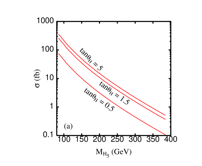
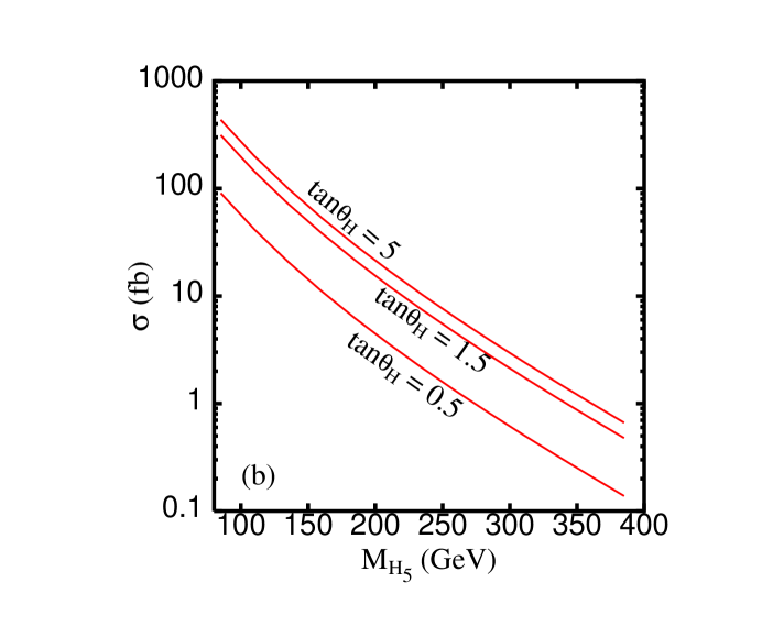
Figure 1: Total production cross sections for (a) $p\bar{p}\to W^{+}H_{5}^{-}+W^{-}H_{5}^{+}$ and (b) $ZH_{5}^{+}+ZH_{5}^{-}$ for $\tan\theta_{H}=0.5,1.5,5$ at $\sqrt{s}=2$ TeV.

The subprocess cross sections are then convoluted with the parton distribution functions to obtain the total production cross sections. Throughout our analysis we use the CTEQ5L distribution set [22]. In Fig. 1, we show the total production cross sections for $W^{+}H_{5}^{-}+W^{-}H_{5}^{+}$ (a) and $ZH_{5}^{+}+ZH_{5}^{-}$ (b) as a function of $M_{H_{5}}$ for three choices of $\tan\theta_{H}=0.5,\,1.5$, and $5$. The cross section increases substantially from $\tan\theta_{H}=0.5$ to $1.5$, but only slightly from $\tan\theta_{H}=1.5$ to $5$. This can be easily understood by the explicit dependence on $\sin\theta_{H}$, as shown in Eq. (11).

The next concern in our analysis is the decay channels and various backgrounds. Since the number of combinations in the decays are quite complicated, we will demonstrate with the best decay channel and the corresponding backgrounds.

Since we are mainly interested in the $W^{+}Z$ decay mode of $H_{5}^{+}$ and we want to have a fully-reconstructed Higgs mass, we would choose the following decay mode of the $H_{5}^{+}$

$$H_{5}^{+}\to W^{+}\;Z\to(q\bar{q}^{\prime})\;(\ell^{+}\ell^{-})\;.$$ (12)

We have assumed that $H_{5}^{+}\to W^{+}Z$ with a 100% branching ratio, which is made possible by adjusting the parameters $\lambda_{4}$ and $\lambda_{5}$ of Eq. (7). The combined branching ratio for the channel in Eq. (12) is about $0.7\times 0.068=0.048$, which takes into account both the electron and muon modes of the $Z$ decay. The branching ratio would increase if we chose the hadronic mode of the $Z$, but it would make the jet combinatorics too complicated for a clean reconstruction. The decay mode of the associated $W$ or $Z$ boson can be either leptonic or hadronic. Therefore, we have the following modes in the final state

$$WH_{5}^{\pm}\to W\;(WZ^{*}/W^{*}Z)\to\left\{\begin{array}[]{c}(\ell\nu)\;(q\bar{q}^{\prime})\;(\ell^{+}\ell^{-})\\ (q\bar{q}^{\prime})\;(q\bar{q}^{\prime})\;(\ell^{+}\ell^{-})\end{array}\right.\;,$$ (13)

and

$$ZH_{5}^{\pm}\to Z\;(WZ^{*}/W^{*}Z)\to\left\{\begin{array}[]{c}(\ell^{+}\ell^{-})\;(q\bar{q}^{\prime})\;(\ell^{+}\ell^{-})\\ (q\bar{q})\;(q\bar{q}^{\prime})\;(\ell^{+}\ell^{-})\end{array}\right.\;,$$ (14)

where “*” denotes an offshell vector boson. These channels result in $3\ell+2j+\not{\!E}_{T}$, $2\ell+4j$, or $4\ell+2j$ in the final state. The signal is a $\alpha_{w}^{2}$ process.

The irreducible backgrounds come from [23]

$$p\bar{p}\to W^{+}W^{-}Z,\;ZW^{\pm}Z,\;ZZZ\;,$$ (15)

which are $\alpha_{w}^{3}$ processes. Thus, before imposing any cuts, these backgrounds are already subdominant relative to the signal. The cross sections for $W^{+}W^{-}Z$, $ZW^{\pm}Z$, and $ZZZ$ at the 2 TeV Tevatron are $6.2$, $1.6$ and $0.6$ fb, respectively. We therefore do not impose specific cuts to suppress these backgrounds, except for the selection cuts for leptons and jets.

Other reducible backgrounds include $W+$jets, $Z+$jets, $WW+$jets, $ZZ+$jets, and $WZ+$jets [24]. The $V+$jets ($V=W,Z$) are $\alpha_{w}\alpha_{s}^{n}$ processes whose cross sections can be, in principle, larger than the signal cross sections. However, they can be reduced substantially by imposing a transverse momentum ($p_{T}$) cut on the jets and by requiring a pair of the jets reconstructed at the $W$ or $Z$ mass. Note that the jets of the signal that come off from the $H_{5}^{+}$ decay have a relatively much larger $p_{T}$. The $VV+$jets ($V=W,Z$) are $\alpha_{w}^{2}\alpha_{s}^{n}$ processes, which are already suppressed relative to the signal.

Next we describe our analysis in details. We apply a typcial resolution [25]

$$\frac{\Delta E}{E}=\frac{0.3}{\sqrt{E}}\oplus 0.01$$ (16)

for leptons, where $E$ is in GeV, and

$$\frac{\Delta E}{E}=\frac{0.8}{\sqrt{E}}\oplus 0.05$$ (17)

for jets. We impose the following selection cuts on leptons and jets [25]

$$p_{T}(\ell) > 10\;{\rm GeV}\;,$$

$$p_{T}(j) > 15\;{\rm GeV}\;,$$

$$\left|\eta_{\ell}\right| < 2.5\;,$$

$$\left|\eta_{j}\right| < 2.5\;,$$

$$\Delta R_{jj} > 0.7\;,$$

$$\Delta R_{\ell j} > 0.4\;,$$

$$\not{\!E}_{T} > 20\;{\rm GeV}\;\;\mbox{when considering $W\to\ell\nu$}\;.$$

From the above discussion we see that the final state of the signal consists of $3\ell+2j+\not{\!E}_{T}$, $2\ell+4j$, or $4\ell+2j$. Let us first concentrate on the $2\ell+4j$ mode because of its largest branching ratio. We shall comment on the other two modes later. In the $2\ell+4j$ mode, there are a few combinations to determine the $2\ell+2j$ that decay from the $H_{5}^{+}$. We employ the following procedures to select the right combination.

First, we reconstruct the associated $W$ or $Z$ boson by demanding that

$$|M_{jj}-M_{Z}| < 10\;{\rm GeV}\,,\;\;\;$$

$$|M_{jj}-M_{W}| < 10\;{\rm GeV}\,,\;\;\;{\rm or}\;\;\;$$

$$|M_{\ell\ell}-M_{Z}| < 10\;{\rm GeV}\,,$$ (18)

where the $2j$ can come from a $W$ or a $Z$ boson while $2\ell$ can only come from the $Z$ boson. It could happen that more than one jet or lepton pair satisfy Eq. (18). In this case, we choose the pair that has a higher transverse momentum $p_{T}$, because we expect that the associated $W$ or $Z$ boson has a higher $p_{T}$ than the boson decaying from the $H^{+}_{5}$. For illustration we show in Fig. 2 the normalized transverse momentum distributions for the associated $W$ and for the $W$ decaying from $H_{5}^{\pm}$ in the $W^{\mp}H_{5}^{\pm}$ production. From the figure it is easy to see that when we select the reconstructed vector boson with a higher transverse momentum, we are more likely to pick the correct associated vector boson. Once we select the correct associated vector boson, we can then reconstruct the invariant mass of the other particles in the final state to form the $H_{5}^{+}$. In Fig. 3, we show both the theoretical $H_{5}^{+}$ mass peaks and the peaks formed by the above procedures. It is clear that our procedures can select the right combination most of the time.

We apply exactly the same procedures to the backgrounds. In the backgrounds, all three vector bosons are on equal footing. Our reconstruction procedures will not select any particular one. The reconstructed spectrum of $jj\ell\ell$ would not show any peak structures but a continuum. In Fig. 4, we show both the background spectrum and the signal peaks for various $H_{5}^{+}$ masses. The background spectrum includes contributions from $WWZ,ZWZ$, and $ZZZ$. Similarly, we have added contributions from $W^{\pm}H_{5}^{\mp}$ and $ZH_{5}^{\pm}$ in the signal. It is obvious that the background is almost negligible under the Higgs peaks. Therefore, the criteria for a discovery of $H_{5}^{+}$ depends crucially on the number of signal events. We require a minimum of 5 events for the evidence of existence. In Table 1, we show the signal cross sections in fb for the signals of $W^{\pm}H_{5}^{\mp}+ZH_{5}^{\pm}$ in the $2\ell+4j$ mode. Given an integrated luminosity of 20 fb^-1 accumulated in the Run 2b of the Tevatron, the sensitive range of $H_{5}^{+}$ is between 110 and 200 GeV. The cross section for $M_{H_{5}^{+}}\approx 100$ GeV is small because of the $p_{T}$ cuts on the leptons and jets that decay from the $H_{5}^{+}$. The heavier the Higgs boson the larger is the $p_{T}$ of its decay products.

5 conclusions

The spectacular signal of the existence of $H_{5}^{\pm}$ is its decay into a $WZ$ pair. We chose the $H_{5}^{\pm}$ decay mode $(q\bar{q}^{\prime}\ell^{+}\ell^{-})$ for a clean reconstruction of the $WZ$ pair. Had we chosen the $4j$ mode, it would have been very difficult to be identified as a $WZ$ pair. The $2\ell+4j$ final state gives an interesting level of signal event rates with a negligible background. A minimum requirement of 5 signal events allows the possible evidence of existence of $H_{5}^{\pm}$ between 110 and 200 GeV.

In our analysis, we have not taken into account the QCD corrections to the signal and backgrounds. The QCD correction to the standard model $VH$ production was known to be about 40% at the Tevatron [26]. We expect about the same enhancement to the $VH_{5}^{\pm}$ and $VVV$ production as the QCD correction is independent of the final states. Therefore, the observability of the $H_{5}^{\pm}$ signal improves, may be up to about 210 GeV.

The decay mode of $H_{5}^{+}$, $H_{5}^{+}\to W^{+}Z\to(q\bar{q}^{\prime})(\ell\ell)$, might be mimicked by the SM Higgs signal, $H_{\rm SM}\to ZZ\to(q\bar{q})(\ell\ell)$. Nevertheless, the mass reconstruction of the $W$ boson can help us to distinguish the triplet-Higgs signal from the SM one. The jet resolution given in Eq. (17) is good enough to provide a reasonable $W$-boson identification. Suppose the $W$ boson decays into 2 jets, each of which has an energy about 50 GeV. According to Eq. (17), the $\Delta E$ of each jet is then about 6 GeV. Thus, the $M_{jj}$ mass resolution is about 8.5 GeV, which is better than the mass difference between the $W$ and the $Z$ bosons.

The other two decay modes $3\ell+2j+\not{\!E}_{T}$ and $4\ell+2j$ would result in an even smaller event rate. That was the reason why we did not pursue it further. Finally, the $WH_{5}^{\pm}\to W\,(W^{\pm}Z)\to(\ell\nu)(jjjj)$ mode suffers from immense background from $t\bar{t}$ production.

In our analysis, the background estimation is based on the on-shell production approximation. If we had taken the vector bosons off-shell, there would have been a small tail at the small invariant mass region in the background curve in Fig. 4. However, this tail is suppressed by $\alpha_{w}$ relative to the on-shell production. Thus, it is negligible compared to the Higgs signal peaks.

There are other continuum backgrounds that we have not taken into account, e.g., $VV+$jets and $V+$jets. We believe that they are suppressed, as we have mentioned earlier, by our cuts to a level even smaller than the background that we have considered in this work.

Table 1: Signal cross sections in fb for $p\bar{p}\to W^{\pm}H_{5}^{\mp},ZH_{5}^{\pm}$ in the $2\ell+4j$ mode. Cuts and branching ratios have already been included in the cross sections. Event rates are also shown for an integrated luminosity of 20 fb^-1.

$M_{H_{5}^{+}}$ (GeV)	$\sigma(W^{\pm}H_{5}^{\mp})$ (fb)	$\sigma(ZH_{5}^{\pm}$) (fb)	$\sigma(W^{\pm}H_{5}^{\mp}+ZH_{5}^{\pm})$ (fb)	Signal events
100	0.05	0.08	0.13	2.6
110	0.15	0.22	0.37	7.4
120	0.22	0.30	0.51	10
140	0.25	0.35	0.60	12
160	0.20	0.29	0.50	10
180	0.14	0.25	0.38	7.6
200	0.09	0.16	0.25	5.0
210	0.07	0.13	0.20	4.0

Figure 2: Normalized transverse-momentum spectra for the associated $W$ (solid) and for the $W$ (dashed) decaying from $H_{5}^{+}$ in the production of $p\bar{p}\to W^{\mp}H_{5}^{\pm}\to W^{\mp}W^{\pm}Z$ at the 2 TeV Tevatron.

Figure 3: Normalized invariant-mass distributions for various $H_{5}^{+}$ masses in the production of $p\bar{p}\to W^{\mp}H_{5}^{\pm}+ZH_{5}^{\pm}$ at the 2 TeV Tevatron. Both the theoretical peaks (solid) and the reconstructed peaks (dashed) are shown for comparison.

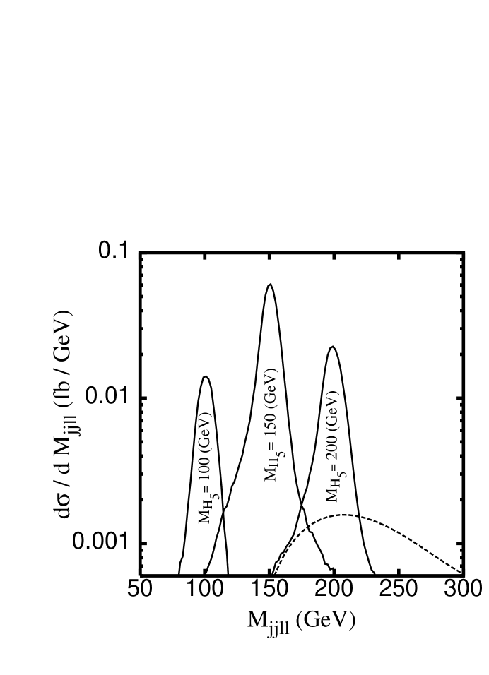
Figure 4: Differential cross section $d\sigma/dM_{jj\ell\ell}$ versus $M_{jj\ell\ell}$ in $p\bar{p}$ collisions at the 2 TeV Tevatron. We show the signal of $W^{\pm}H_{5}^{\mp}+ZH_{5}^{\pm}\to(jj)(jj)(\ell\ell)$ for $M_{H_{5}}=100,150,200$ GeV and $\tan\theta_{H}=1.5$. The continuum background (dashed) from $p\bar{p}\to WWZ,ZWZ,ZZZ$ is also shown.

References

- [1] LEP Higgs Working Group, hep-ex/0107029.
- [2] LEP Higgs Working Group, hep-ex/0107030.
- [3] LEP Electroweak Working Group, LEPEWWG/2002-01.
- [4] J. Gunion, G. Kane, and J. Wudka, Nucl. Phys. B299, 231 (1988).
- [5] M. Peyranère, H. Haber, and P.Irulegui, Phys. Rev. D44, 191 (1991).
- [6] K. Cheung, R. Phillips, and A. Pilaftsis, Phys.Rev. D51, 4731 (1995).
- [7] R.M. Godbole, B. Mukhopadhyaya, and M. Nowakowski, Phys.Lett. B352, 388 (1995).
- [8] D.K. Ghosh, R.M. Godbole, and B. Mukhopadhyaya, Phys. Rev. D55, 3150 (1997).
- [9] R. Vega and D. Dicus, Nucl. Phys. B329, 533 (1990).
- [10] V. Barger, J. Beacom, K. Cheung, and T. Han, Phys. Rev. D50,6704 (1995); R. Alanakian, Phys. Lett. B436, 139 (1998).
- [11] S. Chakrabarti, D. Choudhury, R.M. Godbole, and B. Mukhopadhyaya, Phys. Lett. B434, 347 (1998).
- [12] P. Galison, Nucl. Phys. B232, 26 (1984).
- [13] H. Georgi and M. Machacek, Nucl. Phys. B262, 463 (1985); R. Chivukula and H. Georgi, Phys. Lett. B182, 181 (1986).
- [14] M. Chanowitz and M. Golden, Phys. Lett. B165, 105 (1985).
- [15] J. Gunion, R. Vega, and J. Wudka, Phys. Rev. D42, 1673 (1990); Phys. Rev. D43, 191 (1991).
- [16] A. Akeroyd, Phys. Lett. B442, 335 (1998); Phys.Lett. B353, 519 (1995).
- [17] K. Cheung and D.K. Ghosh, work in progress.
- [18] H. Haber and H. Logan,Phys. Rev. D62, 015011 (2000).
- [19] A. Kundu and B. Mukhopadhyaya, Int. J. Mod. Phys. A11, 5221 (1996).
- [20] M. Ciuchini, G. Degrassi, P. Gambino, and G. Giudice, Nucl. Phys. B527, 527 (1998).
- [21] D. Chakraverty and A. Kundu, Mod. Phys. Lett. A11, 675 (1996).
- [22] CTEQ Collaboration (H. Lai et al.), Eur. Phys. J. C12, 375 (2000).
- [23] V. Barger and T. Han, Phys. Lett. B212, 117 (1988).
- [24] F. Berends, H. Kuijf, B. Tausk, and W. Giele, Nucl. Phys. B357, 32 (1991).
- [25] Future Electroweak Physics at the Fermilab Tevatron: Report of the tev-2000 Study Group, FERMILAB-PUB-96/082, Edited by D. Amidei and R. Brock.
- [26] M. Spira, Fortsch. Phys. 46, 203 (1998); T. Han and S. Willenbrock, Phys. Lett. B273, 167 (1991).
- [27] F. Maltoni and T. Stelzer, hep-ph/0208156.