Abstract

We study the signatures of minimal anomaly mediated supersymmetry breaking in an $e^{-}\gamma$ collider. We demonstrate that the associated production of a sneutrino with the lightest chargino leads to a substantially large signal size. The background is negligibly small, though. Even more interestingly, a measurement of the fundamental supersymmetry breaking parameters could be possible.

PACS NOS. : 12.60.Jv, 13.10.+q, 14.80.Ly

1 Introduction

The question of supersymmetry (SUSY) breaking is of burning relevance in high energy physics today. The most general version of the minimal supersymmetric standard model (MSSM), with the attendant large number of arbitrary SUSY breaking soft parameters, makes itself untractable for experimental searches. However, if the mechanism of SUSY breaking were known, then it would be possible to reduce these large number of parameters into a much smaller set. With the corresponding ordering in the mass spectrum, the nature of the lightest supersymmetric particle (LSP) would be determined, and the decay chains established, thereby making the model much more predictive. Several such supersymmetry breaking mechanisms have been discussed in the literature, alongwith their distinctive phenomenological signatures. Anomaly mediated supersymmetry breaking (AMSB) [1, 2] is one such possibility and has attracted a lot of attention in recent times. Building on the basic idea, wherein the supersymmetry breaking is conveyed to the observable sector by the super-Weyl anomaly, a whole class of models have been constructed [3, 4, 5, 6, 7, 8, 9, 10, 11, 12, 13, 14, 15, 16, 20, 17, 18, 19], and many of the phenomenological implications discussed [5, 16, 21, 22, 23, 24, 25, 26, 27, 28, 29, 30, 31, 32]. For example, the characteristic signatures of the minimal anomaly mediated supersymmetry breaking model (mAMSB) have been studied in the context of hadronic colliders [22, 23, 24, 25, 26, 27, 28, 29], as well as for high energy linear colliders, whether of the $e^{+}e^{-}$ type [30, 31], or photon-photon colliders [32]. In this paper we study the unique signatures of the mAMSB model in an $e^{-}\gamma$ collider.

In its original version, the AMSB scenario consisted of a higher-dimensional supergravity theory wherein the hidden sector and observable sector superfields are localized on two distinct parallel three-branes separated by a distance $\sim r_{c}$ ($r_{c}$ is the compactification radius) in the extra dimension [1]. Below the compactification scale ($\mu_{c}\sim r_{c}^{-1}$), only four-dimensional supergravity fields are assumed to propagate in the bulk. Even if there are additional bulk fields above this scale, their effects would, typically, be suppressed by a factor $e^{-m/{\mu_{c}}}$. As there is no tree level coupling between the hidden sector fields and those in the observable sector, it had been assumed that the flavor changing neutral current (FCNC) processes would be suppressed naturally, thereby solving a longstanding problem of supersymmetric theories. Recently, though, it has been shown that the physical separation between the visible and hidden sectors in extra dimension is not sufficient to suppress the FCNC processes except in some special cases [17]. However, it is possible to construct models of AMSB, even in a completely four-dimensional framework, that can circumvent the flavour problem [18, 19]. For the purposes of the present study, we do not need to delve into such details and would rather be concentrating on the minimal scenario of Ref. [1].

If one were to describe the AMSB scenario in terms of a four-dimensional effective theory, applicable below $\mu_{c}$, then a rescaling transformation can be defined so as to eliminate, from the classical Lagrangian, any tree-level interaction (except for the $\mu$-term in the superpotential) connecting the supergravity fields with the visible sector matter fields. Such a scaling transformation, however, is anomalous and hence supersymmetry breaking is communicated from the hidden sector to the visible sector through the super-conformal anomaly [1]. The supersymmetry breaking soft mass parameters for the gauginos and the scalars are generated at the same order in the corresponding gauge coupling strength. The analytical expressions for the scalar and gaugino masses, in terms of the supersymmetry breaking parameters, are renormalization group (RG) invariant, and, thus, can be computed at the low-energy scale in terms of the appropriate beta functions and anomalous dimensions. The minimal AMSB scenario suffers from a glaring problem though. At low energies, it is beset with the existence of tachyonic sleptons. Several solutions to this problem exist. In this work, we shall consider the minimal AMSB model wherein a constant term $m^{2}_{0}$ is added to all the scalar squared masses thereby making the slepton mass-squareds sufficiently positive. While this may seem to be an ad hoc step, models have been constructed that naturally lead to such an eventuality. A consequence is that the RG invariance of the expression for scalar masses is lost and hence one needs to consider the corresponding evolution down to the electroweak scale.

The minimal AMSB model has several unique features. The gravitino is very heavy, its mass being in the range of tens of TeV. Left and right selectrons and smuons are nearly mass-degenerate while the staus split into two distinct mass eigenstates. But perhaps the most striking feature is that both the lightest supersymmetric particle (LSP) $\widetilde{\chi}_{1}^{0}$ and the lighter chargino ($\widetilde{\chi}_{1}^{\pm}$) are predominantly Winos and hence nearly mass degenerate. Loop corrections as well a small gaugino-Higgsino mixing at the tree level do split the two, but the consequent mass difference is very small: $\Delta M<1{\rm GeV}$. The dominant decay mode of the lighter chargino is $\widetilde{\chi}_{1}^{\pm}\rightarrow\widetilde{\chi}_{1}^{0}+\pi^{\pm}$ and this long-lived chargino would typically result in a heavily ionizing charged track and/or a characteristic soft pion in the detector [33].

Signals of supersymmetry in an $e^{-}\gamma$ collider have been discussed in various contexts [34, 35, 36, 37, 38, 39, 40, 41, 42]. In this paper, we consider the process $e^{-}\gamma\rightarrow\tilde{\nu}\widetilde{\chi}_{1}^{-}$ to look for signals of anomaly mediated supersymmetry breaking in such a collider. This choice has some advantages over the possibilities at an $e^{+}e^{-}$ collider. The dominant production channel at the latter machine, namely a $\tilde{\chi}_{1}^{+}\tilde{\chi}_{1}^{-}$ pair, is notoriously difficult to tag onto, and even if detected, is hardly amenable to mass determination. And as the sleptons tend to be significantly heavier than $\tilde{\chi}_{1}^{+}$, at least for a very large part of the parameter space, the $\tilde{\nu}\widetilde{\chi}_{1}^{-}$ threshold tends to be quite a bit lower than those for $\tilde{\ell}^{+}\tilde{\ell}^{-}$ or $\tilde{\nu}\tilde{\nu}^{*}$. Moreover, the cross section for the first-mentioned process is, generically, much higher, and even more so close to the production threshold.

Once produced, the sneutrino may decay into either an ($e^{-}\tilde{\chi}_{1}^{+}$) pair or a ($\nu\tilde{\chi}_{1}^{0}$) pair. Concentrating upon the former, we are left with a fast $e^{-}$ (which serves as the trigger), two heavily ionizing charged tracks coming from the long-lived $\widetilde{\chi}_{1}^{\pm}$ and/or two visible soft pions with opposite charges and a large missing transverse momentum ($p_{T}/\;\>$). This is a very unique and distinct signature of anomaly mediated supersymmetry breaking and does not readily arise in either of mSUGRA or GMSB scenarios.

What of other channels at an $e^{-}\gamma$ collider itself? Continuing with the same production process, had the selectron decayed into the alternate channel, namely a ($\nu\tilde{\chi}_{1}^{0}$) pair, we would have been left with $\pi^{-}+p_{T}/\;\>$ final state, possibly associated with a single heavily ionized track. The lack of a reliable trigger renders this channel of little use. The associated production of a left selectron and the lightest neutralino ($e^{-}\gamma\rightarrow\tilde{e}_{L}\widetilde{\chi}_{1}^{0}$), on the other hand, would result in the same signal ($e^{-}+p_{T}/\;\>$) as in the case of mSUGRA. Though eminently detectable, this is of hardly any use in establishing the nature of supersymmetry breaking, and hence we desist from discussing it any further. It is, of course, true that, for some choices of the SUSY parameters, the selectron may also decay into the heavier neutralinos ($\tilde{e}_{L}\rightarrow e^{-}\widetilde{\chi}_{2}^{0}$) thereby leading to final states with multifermions and $p_{T}/\;\>$. However, the signal cross section in this case will be small on account of the suppressions due to the various branching ratios. And finally, one may also consider associated production of heavier charginos (with sneutrino) and neutralinos (with selectron) and their subsequent cascade decays. The signals for such processes would be rather complex, though. And the production cross sections typically smaller, both on account of reduced phase space as well as smaller couplings. It may, thus, be said that the channel of our choice is the simplest as well as the most promising one.

The paper is organized as follows. In Sec.2, we give a brief description of the $e^{-}\gamma$ collider. Sec.3 discusses the spectrum and the couplings within the mAMSB model and the constraints on the parameter space from various experimental and theoretical considerations. Numerical results of our computations and their discussions are presented in Sec.4. In Sec.5, we discuss the possibility of determining the supersymmetry breaking parameters. Finally, we conclude in Sec.6.

2 $e^{-}\gamma$ collider and the photon spectrum

While it is quite apparent that maximizing the signal cross sections implies using perfectly polarized electron and photon beams, in reality, though, perfect polarizations is almost impossible. Furthermore, even near monochromaticity for high energy photon beams is extremely unlikely. In fact, the only known way to obtain very high energy photon beams is to induce laser back-scattering off an energetic $e^{\pm}$ beam [43]. The reflected photon beam carries off only a fraction ($y$) of the $e^{\pm}$ energy with

$$\begin{array}[]{rcl}y_{\rm max}&=&\displaystyle\frac{z}{1+z}\\[8.61108pt] z&\equiv&\displaystyle\frac{4E_{b}E_{L}}{m_{e}^{2}}\cos^{2}\frac{\theta_{bL}}{2}\ ,\end{array}$$ (1)

where $E_{b(L)}$ are the energies of the incident electron(positron) beam and the laser respectively and $\theta_{bL}$ is the incidence angle. In principle, one can increase the photon energy by increasing the energy of the laser beam. However, a large $E_{L}$ (or, equivalently, a large $z$) also enhances the probability of electron positron pair creation through laser and scattered-photon interactions, and consequently results in beam degradation. An optimal choice is $z=2(1+\sqrt{2})$, and this is the value that we adopt in our analysis.

The cross-sections for a realistic electron-photon collider can then be obtained by convoluting the fixed-energy cross-sections $\hat{\sigma}({\hat{s}},P_{\gamma},P_{e^{-}})$ with the appropriate photon spectrum:

$$\sigma(s)=\int{\rm d}y\;{\rm d}\hat{s}\;\>\frac{{\rm d}n}{{\rm d}y}(P_{b},P_{L})\;\>\hat{\sigma}({\hat{s}},P_{\gamma},P_{e^{-}})\;\delta(\hat{s}-ys)\ ,$$ (2)

where the photon polarization is itself a function of $P_{b,L}$ and the momentum fraction, viz. $P_{\gamma}=P_{\gamma}(y,P_{b},P_{L})$. For simplicity, we shall only consider circularly polarized lasers scattering off polarized electron (positron) beams. The corresponding number-density $n(y)$ and average helicity for the scattered photons are then given by [43]

$$\begin{array}[]{rcl}\displaystyle\frac{dn}{dy}&=&\displaystyle\frac{2\pi\alpha^{2}}{m_{e}^{2}z\sigma_{C}}C(y)\\[8.61108pt] P_{\gamma}(y)&=&\displaystyle\frac{1}{C(y)}\bigg{[}P_{b}\bigg{\{}\frac{y}{1-y}+y(2r-1)^{2}\bigg{\}}-P_{L}(2r-1)\bigg{(}1-y+\frac{1}{1-y}\bigg{)}\bigg{]}\\[8.61108pt] C(y)&\equiv&\displaystyle\frac{y}{1-y}+(1-y)-4r(1-r)-2P_{b}P_{L}rz(2r-1)(2-y)\ ,\end{array}$$ (3)

where $r\equiv y/z/(1-y)$ and the total Compton cross-section $\sigma_{C}$ provides the normalization.

A further experimental issue needs to be concerned at this stage. While the photon spectrum of eqn.(3) has a long low-energy tail, in a realistic situation it might be that they cannot participate in any interaction. There is a one to one relationship between the energy of the back-scattered photons and their angle with respect to the direction of the initial electron: harder photons are emitted at smaller angles whereas softer photons are emitted at larger angles. For example, for small deflection angles, we have

$$\theta_{\gamma}(y)\simeq{m_{e}\over E_{b}}\sqrt{{z\over y}-z-1}\ .$$ (4)

Since the photons are distributed according to an effective spectrum (eqn.3), this relation effectively throws out the low energy photons, these being produced at too wide an angle to contribute significantly to any interaction. The exact profile of this effective spectrum, though, is not so simple and depends somewhat on the shape of the electron beam, and the conversion distance, i.e. the distance between the interaction point and the point where the laser photons are back-scattered. In the absence of a detailed (and machine specific) study of this effect, we are, unfortunately, not in a position to include it in our simulations. However, as the study of Ref. [38] had indicated, and as we have checked, neglecting this effect does not change the total signal cross section to any significant extent. Elimination of the low energy photons, however, can help in reducing the backgrounds, and thus our approximation is a conservative one.

Before we end this section, we would like to point out that while perfect polarization for the laser beam is relatively easy to obtain, the same is not true for electrons or positrons. In our studies with polarized beams, we shall then use $|P_{L}|=1,|P_{b}|=|P_{e^{-}}|=0.8$ which, once again, reflects a conservative choice. Since we seek to produce the sneutrino, it follows that the $e^{-}$ should be preferentially left-polarized, or $P_{e^{-}}=-0.8$. Similarly, choosing the laser and the $e^{\pm}$ beam to be oppositely polarized ($P_{L}\times P_{b}<0$) improves the monochromaticity of the outgoing photons [44]. For the sake of completeness, we shall use both choices of polarizations consistent with $P_{L}\times P_{b}<0$. While the total cross sections are obviously dependent on the polarization choice, the efficiencis of the kinematical cuts are expected not to be.

3 Model parameters and constraints

The minimal AMSB model has a high degree of predictivity as it is described by just three parameters (apart from the SM parameters, of course): the gravitino mass $m_{3/2}$, the common scalar mass parameter $m_{0}$ and $\tan\beta$, the ratio of the two Higgs vacuum expectation values. In addition, there is a discrete variable, namely the sign of the Higgs mass term ($\mu$). As mentioned earlier, the soft supersymmetry breaking terms in the effective Lagrangian are then determined solely in terms of the gauge ($g_{i}$) and Yukawa ($y_{a}$) couplings. Denoting the generic beta-functions and anomalous dimension by $\beta_{g}(g,y)\equiv dg/dt$, $\beta_{y}(g,y)\equiv dy/dt$ and $\gamma(g,y)\equiv dlnZ/dt$ ($t$ being the logarithmic scale variable) respectively, we have, for the gaugino ($\lambda$) masses

$$M_{\lambda}={\beta_{g}\over g}m_{3/2},$$ (5)

where the appropriate gauge coupling and $\beta$-function are to be considered. Similarly, for the trilinear soft breaking parameters, one has

$$A_{y}={\beta_{y}\over y}m_{3/2}\ .$$ (6)

The scalar masses, on the other hand, receive contributions from more than one source. Apart from the individual contributions from each of the relevant gauge couplings, there is also the universal contribution $m_{0}^{2}$. Symbolically, then,

$$m^{2}_{\tilde{f}}=m^{2}_{0}-{\frac{1}{4}}\sum{\left({{\partial\gamma}\over{\partial g}}\beta_{g}+{{\partial\gamma}\over{\partial y}}\beta_{y}\right)}m^{2}_{3/2}$$ (7)

The detailed expressions for the gaugino masses at the one loop level and the squared masses for the Higgs and the other scalars at the two loop level can be found in Refs. [23, 31, 45].

In our analysis, we use two-loop renormalization group equations (RGE) [46] to evolve the gauge and Yukawa couplings from the unification scale ($M_{G}\sim 2\times 10^{16}$) down to the electroweak scale. For the gauge and Yukawa couplings, the boundary conditions are determined at the weak scale (with $\alpha_{3}(M_{Z})\approx 0.118$), while for the scalar masses these are given at the unification scale vide eqn.(7). The magnitude of the Higgsino mass parameter $\mu$ is computed from the complete one-loop effective potential [47] and imposing the requirement of radiative electroweak symmetry breaking. The optimal choice for the renormalization scale is expressible in terms of the the masses of the top-squarks, viz. $Q^{2}=m_{\tilde{t}_{1}}m_{\tilde{t}_{2}}$. We also include the supersymmetric QCD corrections to the bottom-quark mass [48] since this plays a significant role for large $\tan\beta$.

A particularly interesting feature of the mAMSB model is that the ratios of the gaugino mass parameters, at low energies, turn out to be

$$|M_{1}|:|M_{2}|:|M_{3}|\approx 2.8:1:7.1\ .$$ (8)

In eqn(8), $M_{1}$, $M_{2}$ and $M_{3}$ refer to the $U(1)$, $SU(2)$ and $SU(3)$ gaugino mass parameters respectively. An immediate consequence is that the lighter chargino $\widetilde{\chi}_{1}^{\pm}$ and the lightest neutralino $\widetilde{\chi}_{1}^{0}$ are both almost exclusively a Wino and, hence, nearly degenerate. A small mass difference is generated though from the tree-level gaugino-Higgsino mixing as well as from the one-loop corrections to the chargino and the neutralino mass matrices [23]. The mass splitting has an approximate form:

$$\begin{array}[]{rcl}\Delta M\equiv m_{\tilde{\chi}_{1}^{+}}-m_{\tilde{\chi}_{1}^{0}}&=&\displaystyle\frac{M_{W}^{4}\tan^{2}\theta_{W}}{(M_{1}-M_{2})\mu^{2}}\sin^{2}2\beta\bigg{[}1+{\cal O}\left(\frac{M_{2}}{\mu},\frac{M^{2}_{W}}{\mu M_{1}}\right)\bigg{]}\\[5.16663pt] &+&\displaystyle\frac{\alpha M_{2}}{\pi\sin^{2}\theta_{W}}\bigg{[}f\left(\frac{M_{W}^{2}}{M_{2}^{2}}\right)-\cos^{2}\theta_{W}f\left(\frac{M_{Z}^{2}}{M_{2}^{2}}\right)\bigg{]},\end{array}$$ (9)

with

$$f(x)\equiv-\frac{x}{4}+\frac{x^{2}}{8}\ln(x)+\frac{1}{2}\left(1+\frac{x}{2}\right)\sqrt{4x-x^{2}}\;\tan^{-1}\left(\frac{(1-x)\sqrt{4x-x^{2}}}{3x-x^{2}}\right)\ .$$ (10)

For the range of $m_{0}$ and $m_{3/2}$ that we would be considering in our analysis, $\Delta M\>\raisebox{-2.15277pt}{$\stackrel{{\scriptstyle\textstyle<}}{{\sim}}$}\>$ 500 MeV. And, for very large $M_{2}$, the mass difference reaches an asymptotic value of $\approx$ 165 MeV.

To determine the parameter space allowed to the theory, several experimental constraints need to be considered, the most important ones being:

• $\tilde{\chi}_{1}^{0}$ must be the LSP;

• $m_{\widetilde{\chi}_{1}^{\pm}}>$ 86 GeV, when this chargino almost degenerate with the lightest neutralino [49].

The last constraint serves to rule out relatively low values of $m_{3/2}$ irrespective of the value of $m_{0}$. The width of this disallowed band depends, of course, on $\tan\beta$ and $sgn(\mu)$. The first constraint, on the other hand, restricts the parameter space through a linear relation: $m_{3/2}<am_{0}+b$, where the numerical values of the constants $a,b$, depend, once again, on $\tan\beta$ and $sgn(\mu)$. Typically, the maximum possible value of $m_{3/2}$ for a given $m_{0}$ is a decreasing function of $\tan\beta$. Note that the LEP2 constraints on the lighter stau mass, namely $m_{{\tilde{\tau}}_{1}}>82$ GeV [50], are subsumed by the ones listed above. A detailed discussion of such issues can be found in Ref.[45].

Apart from direct bounds, one must also consider the constraints imposed on virtual exchange contributions to low energy observables. The recent measurement of the muon anomalous magnetic moment $(g_{\mu}-2)$ is a case in point. The resultant constraints on the mAMSB model parameters have been considered by several authors [24, 45, 51, 52]. The numerical results of these papers need to be modified though. For one, the light by light hadronic contribution to $(g_{\mu}-2)$ has since been reevaluated resulting in a reversal of the sign of this particular contribution [53] and a consequent reduction of the discrepancy with the SM result. Even more recently, the E821 experiment has published new data that confirms their earlier result while increasing the precision significantly [54]. It must be borne in mind, though, that the calculation of the SM contribution to $(g_{\mu}-2)$ is beset with many remaining theoretical uncertainties, and, hence, any such constraint must be treated with due circumspection. Constraints are also derivable [24, 51, 52] from the measurement of the rare decay rate $\Gamma(B\rightarrow X_{s}\gamma)$, but, once again, they are not too restrictive and many a loophole exists. Additional bounds may exist if one demands that the electroweak vacuum corresponds to the global minimum of the scalar potential [55, 56]. This restriction, however, can be evaded as long as it can be ensured that the local minimum has a life time longer than the present age of the Universe [57].

4 Signal and Backgrounds

As explained in Section 1, we would be focussing on the production process $e^{-}\gamma\rightarrow\tilde{\nu}\widetilde{\chi}_{1}^{-}$. The sneutrino may subsequently decay into a ($e^{-}+\widetilde{\chi}_{1}^{+}$) pair or through the invisible ($\nu_{e}+\widetilde{\chi}_{1}^{0}$) channel with the branching fractions BR$(\tilde{\nu}_{e}\rightarrow\nu_{e}+\widetilde{\chi}_{1}^{0})\approx 33\%$ and BR$(e^{-}+\widetilde{\chi}_{1}^{+})\approx 66\%$ relatively well determined on account of the $\widetilde{\chi}_{1}^{+}$ and the $\widetilde{\chi}_{1}^{0}$ being predominantly Winos. Decays into the heavier charginos(neutralinos) are kinematically forbidden over most of the parameter space and, even if they are allowed, the branching ratios in those channels are very small. And while three body decays of the form $\tilde{\nu}\rightarrow e^{-}\nu_{\tau}{\tilde{\tau}}^{+}_{1}$ are allowed in principle, in practice they are too small to be of any relevance. For reasons of detectability, we choose to neglect the invisible channel and concentrate on the electron-chargino one. The two charginos subsequently decay into a neutralino-pion pair each. The entire schematics of the signal is presented in Fig. 1. In subsequent discussions, we shall denote $\tilde{\chi}^{-}_{1}$ as the primary chargino and $\tilde{\chi}^{+}_{1}$ (arising from the decay of $\tilde{\nu}$) as the secondary chargino.

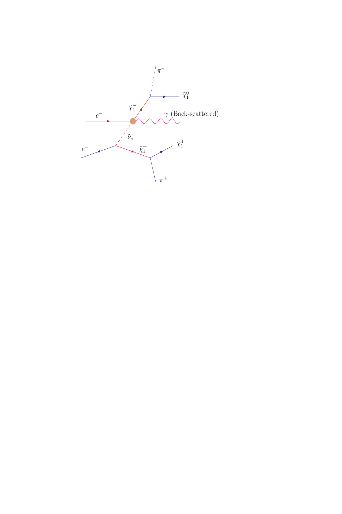
Figure 1: Schematic diagram for the signal process $e^{-}\gamma\to\tilde{\nu}_{e}\tilde{\chi}^{-}_{1}\to e^{-}+\pi^{+}\pi^{-}+p_{T}/\;\>$. We define $\tilde{\chi}^{-}_{1}$ as the primary chargino and $\tilde{\chi}^{+}_{1}$ as the secondary one.

It turns out that, for most of the mAMSB parameter space, the two charged pions are well separated from each other. In particular, when $m_{\tilde{\chi}^{-}_{1}}$ is small compared to both $\sqrt{s}_{e\gamma}$ and $m_{\tilde{\nu}_{e}}$, the boosts imparted to the charginos make the pions appear almost back-to-back. The neutralinos, on the other hand, escape detection, thereby giving rise to an imbalance in momentum.

The signal, then is,

$$e^{-}\gamma\rightarrow\tilde{\nu}_{e}\tilde{\chi}^{-}_{1}\rightarrow e^{-}+\pi^{+}\pi^{-}+p_{T}/\;\>\ ,$$ (11)

with the energetic electron serving as the trigger for the event. The relatively small decay width of the charginos is manifested in heavily ionizing charged tracks (one for each chargino) terminating inside the detector after traversing a macroscopic distance and ending in a soft pion (with $p_{T}>200$ MeV) in the Silicon Vertex Detector (SVD) located very close to the beam pipe. The probability that the chargino decays before travelling a distance $\lambda$ is given by $P(\lambda)=1-exp(-\lambda/L)$, where $L=c\tau(\beta\gamma)$ is the average decay length of the chargino. Although a large fraction of the events do turn out to be associated with a $\tilde{\chi}^{\pm}_{1}$ decay that is so prompt as to make the charged track nearly invisible (the end product—soft $\pi$—is still detectable), a substantial number of events do have a reasonably large decay lengths for which the displaced vertex $X_{D}$ may be visible. Consequently, one could find a thick ionizing charged track in the first few layers of the SVD with the track terminating to give off a soft pion, which can be observed through its impact parameter. In the worst case, when the chargino track is not seen, our signal can still be observed by looking at the soft pion impact parameter $b_{\pi}$.

We select the signal events according to the following criteria:

• The transverse momentum of the electron must be large enough: $p^{e}_{T}>20$ GeV.

• The transverse momentum of the pions must satisfy $p^{\pi}_{T}>0.2\>\rm GeV$.

• The total energy of the pions should not be very large though: $E^{\pi}<2\>\rm GeV$.

• The electron and both the pions must be relatively central, i.e. their pseudorapidities must fall in the range $\mid\eta^{e,\pi}\mid<2.5$.

• The electron and the pions must be well-separated from each other: i.e. the isolation variable $\Delta R\equiv\sqrt{(\Delta\eta)^{2}+(\Delta\phi)^{2}}$ (where $\eta$ and $\phi$ denote the separation in rapidity and the azimuthal angle respectively) should satisfy $\Delta R>0.4$ for each combination.

• The missing transverse energy $p_{T}/\;\>>20$ GeV.

Any heavily ionizing charged track would be an additional bonus. While the rationale behind most of the kinematical requirements listed above is self-evident, the importance of the upper bound on the pion energy would become clear shortly.

4.1 The SM background

Before we discuss the ensuing signal cross section, let us first examine the possible Standard Model backgrounds. This would also help put into perspective the cuts listed above. A heavily ionizing track may arise only from the motion of a relatively massive charged object. The only particles in the SM spectrum that fit the bill are ones that decay promptly (and hence leave no ionizing track). Thus, if macroscopic tracks are seen , the signal is essentially free of backgrounds.

What if no tracks are seen at all? The signal then comprises of just a hard electron and two soft pions and accompanied by a measure of missing energy. The backgrounds to this are manifold:

• $e^{-}\gamma\to e^{-}\pi^{+}\pi^{-}\nu_{i}\bar{\nu}_{i}$: While an accurate calculation of this is a difficult task, a fair estimate may be made by the use of scalar-QED (as well as scalar QFD). To improve accuracy, form factors may be used to parametrize the vertices involving the pions. It is here that the upper bound on the pion energy, as discussed above, assumes importance. Since the pion-photon vertices (as well as the pion-$Z$ or pion-$W$ vertices) arise from derivative couplings, a process such as the one we are describing would be heavily biased towards energetic pions. With the cuts that we have imposed, the total cross section of this particular background is $\>\raisebox{-2.15277pt}{$\stackrel{{\scriptstyle\textstyle<}}{{\sim}}$}\>{\cal O}(10^{-3}\>\rm fb)$ and hence entirely negligible.

• $e^{-}\gamma\to e^{-}q\bar{q}\nu_{i}\bar{\nu}_{i}$ with the quarks hadronizing into soft pions:
  The largest contribution to the partonic process accrues from the production mode $e^{-}\gamma\to e^{-}ZZ$ with a $Z$ each decaying into quarks and neutrinos. It is easy to see that the quarks from such processes would be very energetic and would not lead to just a pair of soft pions unaccompanied by any other hadronic activity. As for the continuum process $e^{-}\gamma\to e^{-}q\bar{q}Z$ (with $Z\rightarrow\nu_{i}\bar{\nu}_{i}$), it is a ${\cal O}(\alpha_{W}^{4})$ one and hence highly suppressed.
  It is often argued that a signal with just a pair of soft pions, an electron trigger and no macroscopic ionization track would suffer from large, and almost incalculable, QCD backgrounds. However, as explained above, the particular electroweak process that can give rise to a event topology similar to our signal, is highly suppressed and even non-perturbative QCD corrections cannot enhance it to significant levels.

• $e^{-}\gamma\to e^{-}\tau^{+}\tau^{-}$ with the taus decaying appropriately:
  While estimating this background, it is imperative that the $\tau$-polarization information be retained in the intermediate stages of the calculation, especially since the distribution of the decay products depend crucially on the polarization. We include all decay channels that involve two charged pions satisfying our selection criteria. Since some of the events thus included may be vetoed by other criteria (such as the absence of a $\pi^{0}$), our choice is a conservative one. On imposition of our cuts, the surviving background is $\>\raisebox{-2.15277pt}{$\stackrel{{\scriptstyle\textstyle<}}{{\sim}}$}\>0.05\>\rm fb$, with the exact numbers depending on the polarization choice.

• $e^{-}\gamma\to e^{-}W^{+}W^{-}$ with $W\to\tau\to\pi$ :
  While the $W$-pair production cross section is sizeable, the $\tau$’s and hence the $\pi$’s tend to be harder. This serves to suppress the background to below ${\cal O}(10^{-3}\>\rm fb)$.

4.2 The signal profile

As we have seen in the previous section, we may safely conclude that, even in the absence of macroscopic ionization tracks, our selection criteria serves to remove virtually all of the SM background. What of the signal, then? Clearly, both the number of signal events and the kinematical distributions thereof would depend crucially on the sneutrino and chargino mass. We will illustrate the case for two widely separated points in the parameter space:

• $m_{0}=210\>\rm GeV,m_{3/2}=37\>\rm TeV,\tan\beta=5$ and $\mu>0$
  which leads to $(m_{\widetilde{\chi}_{1}^{+}},m_{\widetilde{\chi}_{1}^{0}},m_{\tilde{\nu}})=(119.64,119.39,139.11)\>\rm GeV$; and

• $m_{0}=450\>\rm GeV,m_{3/2}=55\>\rm TeV,\tan\beta=30$ and $\mu>0$
  leading to $(m_{\widetilde{\chi}_{1}^{+}},m_{\widetilde{\chi}_{1}^{0}},m_{\tilde{\nu}})=(186.42,186.23,390.07)\>\rm GeV$.

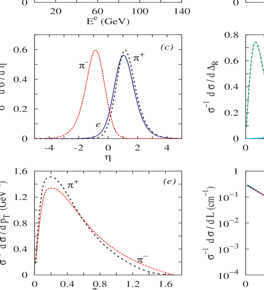
Figure 2: Normalized kinematic distributions of signal events at a machine operating with $\sqrt{s}_{ee}=1\>\rm TeV$ and beam polarization choices: $P_{L}=-1.0,P_{b}=0.8,P_{e^{-}}=-0.8$. The AMSB parameters are $m_{0}=210~{}{\rm~{}GeV},m_{3/2}=37~{}{\rm~{}TeV},tan\beta=5,sgn(\mu)>0$ (point A). The different panels correspond to (a) electron energy; (b) electron $p_{T}$; (c) rapidities; (d) cone separations (e) pion $p_{T}$s; and (f) chargino decay lengths.

Let us concentrate, for the moment, on the parameter space point (A). Had we a monochromatic photon beam, the sneutrino and the chargino would have been monochromatic too. And since the electron is a product of the two-body decay of the sneutrino into the very same chargino, the electron energy would have been strictly bound on both sides (with the bounds determined by $m_{\tilde{\nu}}$ and $m_{\widetilde{\chi}_{1}^{+}}$), and the distribution uniform within. Although this simplistic situation is modified to a degree by the spread in the photon spectrum, the main feature is still quite discernible (see Fig. 2a). The transverse momentum of the electron (see Fig. 2b), too, shows unmistakable signs of its kinematic origin, with the position of the peak being governed, once again, by $m_{\tilde{\nu}}$ and $m_{\widetilde{\chi}_{1}^{+}}$. With its rapidity distribution mirroring that of the sneutrino, the electron is still relatively central, though boosted in the direction of the incoming electron beam (Fig. 2c). The same holds for the $\pi^{+}$ arising from the sneutrino decay. The $\pi^{-}$, on the other hand, is a decay product of the primary chargino ( $\tilde{\chi}^{-}_{1}$) and is hence boosted somewhat in the direction of the incoming photon beam (Fig. 2c). This immediately suggests that the $\pi^{-}$ would be well separated from both the electron and the $\pi^{+}$, a conclusion supported by the distribution displayed in Fig. 2d. Once again, this conclusion holds almost over the entire SUSY parameter range under consideration. The angular separation between the electron and the $\pi^{+}$, on the other hand, is a sensitive function of the difference $m_{\tilde{\nu}}-m_{\widetilde{\chi}_{1}^{+}}$ and, for larger mass differences, peaks at larger values. Of crucial importance are the transverse momenta of the pions, for a minimal value is necessary for them to be detected. As expected, the pions are very soft (see Fig. 2e), with the extent of the $p_{T}$ (as well as energy) distributions determined by $m_{\widetilde{\chi}_{1}^{+}}-m_{\widetilde{\chi}_{1}^{0}}$. The very same quantity (alongwith the absolute magnitude of the masses) also determine the decay length of the charginos. The slightly faster decay of the primary chargino in this case (see Fig. 2f) is but a reflection of its having a lower average momentum.

( $m_{0}~{}{\rm(GeV)},~{}m_{3/2}~{}{\rm(TeV)},\tan\beta$ )	A.     (210, 37, 5)			B.     (450, 55.0, 30)
( $m_{\tilde{\chi}^{+}_{1}},m_{\tilde{\chi}^{0}_{1}},m_{\tilde{\nu}}~{})~{}{\rm(GeV)}$	( 119.64, 119.39, 139.11 )			( 186.42, 186.23, 390.07)
	$(P_{L},P_{b},P_{e^{-}})$			$(P_{L},P_{b},P_{e^{-}})$
	($-,+,-$)	($+,-,-$)	($0,0,0$)	($-,+,-$)	($+,-,-$)	($0,0,0$)
Total $\sigma$ (fb)	407.1	279.3	169.3	139.3	201.9	82.3
$|\eta_{e}|<2.5$	386.7	250.9	157.0	136.5	197.0	80.4
$p_{T}^{e}>20$ GeV	265.5	144.5	100.6	136.1	196.4	80.2
Both $|\eta_{\pi}|<2.5$	248.7	125.5	91.6	130.7	183.2	75.9
Both $p_{T}^{\pi}>200$ MeV	179.6	79.5	63.1	30.6	32.3	14.4
$\Delta_{e\pi}>0.4$	125.5	59.5	45.7	30.3	32.0	14.2
$\Delta_{[\pi_{1}\pi_{2}]}>0.4$	125.5	59.5	45.7	30.3	32.0	14.2
$p_{T}/\;\>>20$ GeV	125.0	59.0	45.4	30.1	32.0	14.2
Decay length for one chargino $>$ 4.0 cm	62.5	28.9	21.8	22.1	22.2	9.68
Decay length for both chargino $>$ 4.0 cm	10.7	4.6	3.48	6.9	6.37	2.70

Table 1: Illustrating the effects of various cuts on the signal cross-sections for two specimen points in the parameter space and for $\sqrt{s}_{ee}=1$ TeV. In either case, $\mu>0$, and the cross sections are shown both for unpolarized beams as well as for two particular choices for beam polarizations. Whenever nonzero, $|P_{L}|$ = 1 and $|P_{b}|=|P_{e^{-}}|=0.8$.

Having discussed the kinematics, it is now relatively easy to anticipate the effects of the cuts that we have chosen to impose. As we shall shortly see, the efficiency has a nontrivial dependence on the superparticle masses. While, in an actual experimental context, it might be more prudent to employ flexible cuts, we shall, nevertheless, continue to work with those that we have already described. As Table 1 shows, the requirement on the minimum electron transverse momentum serves to reject quite a few signal events for a small $m_{\tilde{\nu}}$ and/or a small difference $m_{\tilde{\nu}}-m_{\widetilde{\chi}_{1}^{+}}$. Were both these to be large (point B), the effect is marginal at best. A similar statement may also be made for the angular separation between the electron and the $\pi^{+}$. On the other hand, a small mass difference between the chargino and neutralino renders the requirement on the pion transverse momentum a crucial one (a larger fraction of the signal is lost for point B than for point A). And, as expected, the rest of the cuts imposed have only marginal effect on the signal. Finally, a remark on the chargino track lengths. As shown in Table. 1, if we insist that both charginos leave a substantial track, we would be discarding the majority of events. While this may still be fine for relatively lighter superparticles, when the cross sections are large, such a requirement would severely limit the reach of the experiment. In view of our demonstration that our signal is relatively background-free even in the absence of macroscopic tracks, it is perhaps unnecessary to impose such a requirement, at least in the discovery stage. Of course, if a signal were to appear, one could always go back and look for the confirmatory tracks. This is the standpoint we shall adopt in the remainder of the article.

4.3 Signal strength and the parameter space

Until now, we have restricted ourselves to an examination of the signal profile for two specific points in the parameter space. While the gross features can be inferred from the discussion in the previous section, it is of interest to determine magnitude of the total signal strength as a function of the parameters involved. We aim to do this now. Clearly, it is not possible to depict the dependence on each of the parameters, and hence we shall restrict ourselves to two discrete values of $\tan\beta$ while allowing $m_{0}$ and $m_{3/2}$ to vary freely modulo the experimental constraints. As for the beam polarization, we make a particular choice, namely $P_{L}=+1,P_{b}=P_{e^{-}}=-0.8$.

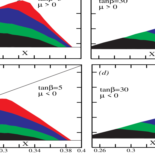
Figure 3: Scatter plots for the signal cross-section (fb) in the $m_{0}-m_{3/2}$ plane for a machine operating at $\sqrt{s}_{ee}=500\>\rm GeV$ and $P_{L}=+1,P_{b}=P_{e^{-}}=-0.8$. The values of $tan\beta$ and $sgn(\mu)$ are as indicated. The regions marked by $X$ are ruled out by the experimental lower limit on the chargino mass, while those marked by $Y$ are ruled out by the requirement of $\widetilde{\chi}_{1}^{0}$ being the LSP. In each panel, the top three shaded regions correspond to cross section ranges of $[(0.1-5),~{}(5-50),~{}(50-150)]$. The lowermost region corresponds to $(150-470)$ in ${\em(a)}$, $(150-390)$ in ${\em(b)}$, $(150-335)$ in ${\em(c)}$ and $(150-350)$ in ${\em(d)}$ respectively.

In Fig.3, we display our results for a machine operating at $\sqrt{s}_{ee}=500\>\rm GeV$, in the form of scatter plots for the cross section, after imposing the cuts, in the plane spanned by $m_{0}$ and $m_{3/2}$. The panels on the left(right) correspond to low (high) $\tan\beta$ (5 and 30). For each choice, we also depict the dependence on the sign of the $\mu$-term. In each of the individual graphs, the region marked by $X$ corresponds to a chargino mass of less than 86 GeV, thereby falling foul of the ALEPH bound [49]. The region $Y$, on the other hand, would correspond to the $\tilde{\tau}_{1}$ being the LSP, a possibility not allowed phenomenologically if $R$-parity is to be conserved. We, thus, need to consider ourselves only with the wedge-shaped region enclosed by the two straight lines. Note that the extent of the region $Y$ is much more sensitive to the value of $\tan\beta$ than is the case for the region $X$. This is easy to understand when one considers the fact that a large $\tan\beta$ results in making the $\tau$-Yukawa coupling stronger, which, in turn, drives down the mass of the lighter $\tilde{\tau}$, thereby rendering it the LSP.

It is obvious that the total cross section would fall monotonically with each of the two mass parameters, and this is amply reflected in the figure. Note that the variation with $m_{3/2}$ is much sharper for large $m_{0}$. This, again, is easy to understand as one is progressively squeezing the available phase space for the production process. The variations with $\tan\beta$ and the sign of $\mu$ are of a subtler origin, namely the dependence of $\Delta M$ (the mass-difference between the lighter chargino and the lightest neutralino) on these two parameters. It can be easily ascertained that, for positive $\mu$, the mass-difference $\Delta M$ decreases with $\tan\beta$. This, in turn, implies that the pions resulting from the decay of the chargino have a higher average transverse momentum for lower $\tan\beta$, thereby making them easier to detect. For negative $\mu$, the effect is opposite.

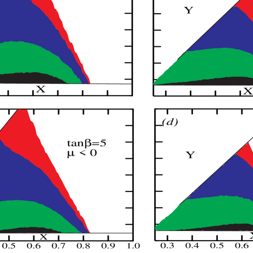
Figure 4: As in Fig.3, but for $\sqrt{s}_{ee}=1\>\rm TeV$ instead. In each panel, the top three shaded regions correspond to cross section ranges of $[(0.1-5),~{}(5-50),~{}(50-150)]$. The lowermost region corresponds to $(150-215)$ in ${\bf(a)}$, $(150-205)$ in ${\bf(b)}$, $(150-185)$ in ${\bf(c)}$ and $(150-195)$ in ${\bf(d)}$ respectively.

It is clear from Fig.3 that, for the low $tan\beta$ case, an experiment such as this can easily explore $m_{3/2}$ as high as $60(50)$ TeV for negative (positive) $\mu$. For $tan\beta=30$, on the other hand, the maximal reach in $m_{3/2}$ is approximately 40 TeV irrespective of $sgn(\mu)$. Similarly, the reach in $m_{0}$ has little dependence on either of $tan\beta$ and $sgn(\mu)$. Finally, it must be borne in mind that Fig.3 has been drawn keeping in mind a moderate luminosity ($\>\raisebox{-2.15277pt}{$\stackrel{{\scriptstyle\textstyle<}}{{\sim}}$}\>100\>\rm fb^{-1}$). A significantly larger integrated luminosity would, of course, allow one to explore beyond the topmost shaded band.

In Fig.4, we show a similar plot for a machine opearting at $\sqrt{s}_{ee}=1\>\rm TeV$ instead. The features are very similar, with the obvious enhancement in the reach.

5 Parameter Determination

Once the existence of a new particle has been confirmed, it is almost contingent upon the experimentalist to determine its mass, spin etc. and, hopefully, glean further information as to the possible values of the parameters within a particular theoretical framework. We shall now investigate the possibility for such studies at an $e\gamma$ collider.

Positing that the particles produced were the sneutrino and the chargino and that the sneutrino subsequently decayed into a similar chargino and an electron, it is easy to see that the energy of the decay electron is strictly confined [38] within the interval

$${m_{\tilde{\nu}}^{2}-m_{\tilde{\chi}_{1}^{+}}^{2}\over 2\left(E_{\tilde{\nu}}^{\rm max}+k_{\tilde{\nu}}^{\rm max}\right)}\leq E^{e}\leq{m_{\tilde{\nu}}^{2}-m_{\tilde{\chi}_{1}^{+}}^{2}\over 2\left(E_{\tilde{\nu}}^{\rm max}-k_{\tilde{\nu}}^{\rm max}\right)}\ ,$$ (12)

where $E_{\tilde{\nu}}^{\rm max}$ is the maximum possible energy that the intermediate sneutrino may have carried, viz.

$$E_{\tilde{\nu}}^{\rm max}={1\over 4y_{\rm max}\sqrt{s}} \Biggl{[} (1+y_{\rm max})\left(y_{\rm max}s+m_{\tilde{\nu}}^{2}-m_{\tilde{\chi}_{1}^{+}}^{2}\right)$$ (13)

$$+ (1-y_{\rm max})\sqrt{\left(y_{\rm max}s+m_{\tilde{\nu}}^{2}-m_{\tilde{\chi}_{1}^{+}}^{2}\right)^{2}-4y_{\rm max}sm_{\tilde{\nu}}^{2}}\quad\Biggr{]}\ ,$$

and $k_{\tilde{\nu}}^{\rm max}$ is the corresponding momentum.

As $\sqrt{s}$ and $y_{\rm max}$ are both known, it follows that an accurate measurement of $E^{e}_{\rm max}$ and $E^{e}_{\rm min}$ would allow us to determine both the masses. A very precise measurement of the endpoints is unlikely, though. The reasons are manifold. Apart from the issue of energy resolution, one has to take into account that the sharp edges, as displayed in Fig. 2a, do not remain as sharp once all the cuts are imposed. Rather, there is a more gradual tapering off at the higher end, as displayed in Fig. 5. This, obviously, could result in an underestimation of $E^{e}_{\rm max}$, and, from a random survey in the parameter space, we find that this effect is typically $\>\raisebox{-2.15277pt}{$\stackrel{{\scriptstyle\textstyle<}}{{\sim}}$}\>20\>\rm GeV$. To account for this, we consider a conservative error contribution of $25\>\rm GeV$ in the measurement of $E^{e}_{\rm max}$.

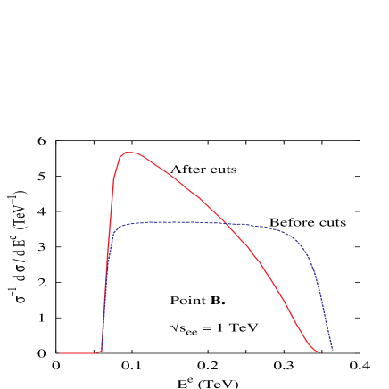
Figure 5: The normalized electron energy distribution for parameter point B (see text). The dashed (solid) lines depict the cross section before (after) all the selection criteria are imposed.

The determination of $E^{e}_{\rm min}$, on the other hand, does not suffer from this problem, and, hence, we only consider an error of $5\>\rm GeV$ to account for the finite resolution. There is a caveat, though. Looking at Fig. 2a (or, equivalently, eqns. 12&13), one immediately sees that the true $E^{e}_{\rm min}$ may very well be less than $20\>\rm GeV$, and hence in contradiction with our requirement on the minimal transverse momentum for the electron. Clearly, for such points in the parameter space, $\delta E^{e}_{\rm min}\>\raisebox{-2.15277pt}{$\stackrel{{\scriptstyle\textstyle>}}{{\sim}}$}\>20\>\rm GeV$. Of course, for a given collider configuration, it is easy to determine the part of the parameter space that is beset with this particular problem. In the rest of this section, we rather concentrate on a point that lies outside this region, namely the point B discussed earlier.

In Fig. 6a, we display the two bands obtained from the measurement of the two electron energy endpoints corresponding to point B. The measurement errors are exactly as described above, and the curious shape of the band is but a consequence of the nonlinear nature of eqn.(12). What is interesting is that the two measurements lead to very different constraints in the parameter space, thereby facilitating a relatively good measurement of the two masses. The error on the sneutrino mass, thus determined, is roughly 12 GeV, while that on the chargino mass is roughly 6 GeV. Moreover, the errors are quite correlated (see Fig. 6b, which displays the region of interest on an expanded scale) and hence the combined $1\sigma$ ellipse would lie well within the overlap region. Note that all this information has been gleaned from a single process and without an energy scanning.

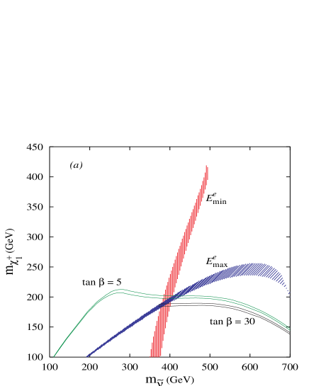
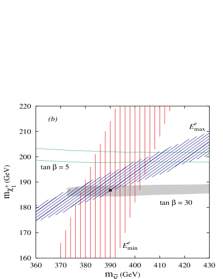
Figure 6: (a) The determination of the sneutrino and chargino masses from a measurement of the endpoints of the electron energy spectrum (eqn.12). The width of the bands correspond to the error bars described in the text. For points within the two horizontal bands, the resultant cross section would agree with the measured one to within $1\sigma$. (b) The overlap region has been shown on an expanded scale. The dark square denotes the reference point in the parameter space (pt. B in the text).

Having determined the masses, it is now of interest to measure the remaining parameter, namely $\tan\beta$. Clearly, kinematical distributions are essentially independent of this quantity and one should rather consider cross section measurement, or, in other words, a counting experiment. For this purpose, we choose to work with a moderate choice of luminosity, viz. ${\cal L}=100\>\rm fb^{-1}$. The cross sections are converted to event numbers through the relation

$$n=\sigma\cdot\epsilon\cdot{\cal L}$$

where the overall detection efficiency $\epsilon$ is but the product of the efficiency for pion detection (assumed to be 50% each) and those for electron detection (95%). The corresponding error in the cross section measurement (after imposing the cuts, naturally) is easily determined on application of Poisson (or Gaussian) statistics. Armed with this, and for a given value of $\tan\beta$, one could easily determine the part of the $m_{\tilde{\nu}}$–$m_{\tilde{\chi}_{1}^{+}}$ space that would be consistent with the measured cross section. In Figs. 6, we display these constraints for two particular values of the ratio $\tan\beta$. One might wonder at the abrupt end for the band corresponding to $\tan\beta=30$. This, however, is but a consequence of the aforementioned constraints on the mass of $\tilde{\tau}_{1}$. Note that, while some resolution is possible, such experiments are not overly sensitive to this parameter. It is possible that significant improvement would occur once other production processes are considered, but that is beyond the scope of the present work.

6 Conclusions

To summarise, we discuss the feasibility of using an electron-photon collider to investigate minimal models wherein supersymmetry breaking is mediated to the visble sector through the super-Weyl anomaly. A very striking feature of such models, including the minimal model we have studied here, is that the lightest chargino $\widetilde{\chi}_{1}^{\pm}$ and the lightest neutralino $\widetilde{\chi}_{1}^{0}$ are nearly degenerate and predominantly Winos. This leads to a long-lived $\widetilde{\chi}_{1}^{\pm}$ which then decays into $\widetilde{\chi}_{1}^{0}+\pi^{\pm}$ (soft) resulting in a heavily ionizing charged track and a soft $\pi^{\pm}$ whose impact parameter may be measurable. While signals for such scenarios have been studied in the context of other colliders, this very feature often restricts the detectability of the model.

We demonstrated though, that the associated production of the lighter chargino and the sneutrino at an $e\gamma$ collider could provide a very clean signature for such a scenario. The signal event consists of an energetic electron (emanating from the decay of the sneutrino) which serves as the trigger, two macroscopic charged tracks in the vertex detector and/or two soft charged pions and, of course, a large missing transverse momentum. The possible SM backgrounds are calculated and shown to be negligibly small once suitable selection criteria are employed. Consequently, even with an integrated luminosity of only $100\>\rm fb^{-1}$, one could see as many as 1000 (background-free) signal events over a very large region of the allowed parameter space.

Additional advantages of the mode we advocate are encapsulated in the kinematic distribution of the signal events. The presence of distinct energy endpoints for the electron allows one to determine the masses of both the chargino and the sneutrino to a fair degree of accuracy. For a very large part of the parameter space, this is true even without an energy scan. The latter technique, if employed, can only improve the measurements. In addition, a measurement of the cross section can be used to constrain the possible range for $\tan\beta$.

Once the signal has been established and all possible information gleaned, the same collider can easily be used to obtain confirmatory checks. The simplest example is the associated production of the left-selectron with the lightest neutralino. A more non-trivial example (and requiring a higher energy) is the associated production of the right-selectron with the second-lightest neutralino. Using techniques similar to those discussed here, one could also measure the masses of these two particles. Since AMSB models have very definite predictions for the ratios of the masses of two lightest neutralinos as well as for the splitting of slepton masses, such tests are likely to be crucial in establishing the mechanism of supersymmetry breaking as well as the parameters of the theory. We hope to come back to this issue in the near future.

Acknowledgments DKG would like thank the Department of Physics, National Taiwan University, Taipei, where the initial part of this work was done. SR thanks Aseshkrishna Datta and Biswarup Mukhopadhyaya for very helpful discussions. DC would like to thank the Dept. of Science and Technology, India for financial assistance under the Swarnajayanti Fellowship grant.

References

- [1] L. Randall and R. Sundrum, Nucl. Phys. B557, 79 (1999).
- [2] G.F. Giudice, M.A. Luty, H. Murayama and R. Rattazzi, J. High Energy Phys. 12, 027 (1998).
- [3] J.A. Bagger, T. Moroi and E. Poppitz, J. High Energy Phys. 04, 009 (2000).
- [4] A. Pomarol and R. Rattazzi, J. High Energy Phys. 05, 013 (1999).
- [5] G.D. Kribs, Phys. Rev. D 62, 015008 (2000).
- [6] E. Katz, Y. Shadmi and Y. Shirman, J. High Energy Phys. 08, 015 (1999).
- [7] I. Jack and D.R.T. Jones, Phys. Lett. B 482, 167 (2000).
- [8] M. Carena, K. Huitu and T. Kobayashi, Nucl. Phys. B592, 164 (2000).
- [9] Z. Chacko, M.A. Luty, I. Maksymyk and E. Ponton, J. High Energy Phys. 04, 001 (2000).
- [10] B.C. Allanach and A. Dedes, J. High Energy Phys. 06, 017 (2000).
- [11] N. Arkani-Hamed, D. E. Kaplan, H. Murayama, Y. Nomura, J. High Energy Phys. 02, 041 (2001).
- [12] Z. Chacko, M.A. Luty, E. Ponton, Y. Shadmi and Y. Shirman, Phys. Rev. D 64, 055009 (2001).
- [13] I. Jack and D.R.T. Jones, Phys. Lett. B 491, 151 (2000).
- [14] D.E. Kaplan and G.D. Kribs, J. High Energy Phys. 09, 048 (2000).
- [15] A.E. Nelson, N. Weiner, Phys. Rev. Lett. 88, 231802 (2002).
- [16] F. de Campos, M.A. Díaz, O.J.P. Éboli, M.B. Magro and P.G. Mercadante, Nucl. Phys. B623, 47 (2002).
- [17] A. Anisimov, M. Dine, M. Graesser and S. Thomas, Phys. Rev. D 65, 105011 (2002); hep-th/0201256.
- [18] M.A. Luty, R. Sundrum, Phys. Rev. D 65, 066004 (2002); hep-th/0111231.
- [19] R. Harnik, H. Murayama and A. Pierce, hep-ph/0204122.
- [20] I. Jack, D.R.T. Jones and R. Wild, Phys. Lett. B 535, 193 (2002).
- [21] R. Rattazzi, A. Strumia and J.D. Wells, Nucl. Phys. B576, 3 (2000).
- [22] J.L. Feng, T. Moroi, L. Randall, M. Strassler and S. Su, Phys. Rev. Lett. 83, 1731 (1999).
- [23] T. Gherghetta, G.F. Giudice and J.D. Wells, Nucl. Phys. B559, 27 (1999).
- [24] J.L. Feng and T. Moroi, Phys. Rev. D 61, 095004 (2000).
- [25] S. Su, Nucl. Phys. B573, 87 (2000).
- [26] F. Paige and J. Wells, hep-ph/0001249.
- [27] H. Baer, J.K. Mizukoshi and X. Tata, Phys. Lett. B 488, 367 (2000).
- [28] A. Datta, P. Konar and B. Mukhopadhyaya, Phys. Rev. Lett. 88, 181802 (2002) (hep-ph/0111012).
- [29] A.J. Barr, C.G. Lester, M.A. Parker, B.C. Allanach, P. Richardson, hep-ph/0208214.
-
[30]
D.K. Ghosh, P. Roy and S. Roy, J. High Energy Phys. 08, 031 (2000);
A. Datta and S. Maity, Phys. Lett. B 513, 130 (2001). - [31] D.K. Ghosh, A. Kundu, P. Roy and S. Roy, Phys. Rev. D 64, 115001 (2001).
- [32] D. Choudhury, B. Mukhopadhyaya, S. Rakshit and A. Datta, hep-ph/0205103.
-
[33]
C.H. Chen, M. Drees, and J.F. Gunion, Phys. Rev. Lett. 76, 2002 (1996); Phys. Rev. D 55, 330 (1997);
Phys. Rev. Lett. 82, 3192(E) (1999);
J.F. Gunion and S. Mrenna, Phys. Rev. D 64, 075002 (2001). - [34] R.W. Robinett, Phys. Rev. D 31, 1657 (1985).
- [35] F. Cuypers, G.J. van Oldenberg, and R. Rückl, Nucl. Phys. B383, 45 (1992).
- [36] H.A. König and K.A. Peterson, Phys. Lett. B 294, 110 (1992).
- [37] T. Kon and A. Goto, Phys. Lett. B 295, 324 (1992).
- [38] D. Choudhury and F. Cuypers, Nucl. Phys. B451, 16 (1995).
- [39] K. Kiers, J.N. Ng and G.H. Wu, Phys. Lett. B 381, 177 (1996).
- [40] V. Barger, T. Han and J. Kelly, Phys. Lett. B 419, 233 (1998).
- [41] A. Ghosal, A. Kundu and B. Mukhopadhyaya, Phys. Rev. D 57, 1972 (1998).
- [42] D. K. Ghosh and S. Raychaudhuri, Phys. Lett. B 422, 187 (1998).
- [43] I. F. Ginzburg, G. L. Kotkin, V. .G. Serbo and V. I. Telnov, Nucl. Instr. Meth. 205, 47 (1983).
- [44] S. Berge, M. Klasen and Y. Umeda, Phys. Rev. D 63, 035003 (2001).
- [45] U. Chattopadhyay, D.K. Ghosh and S. Roy, Phys. Rev. D 62, 115001 (2000).
- [46] S.P. Martin and M.T. Vaughn, Phys. Rev. D 50, 2282 (1994).
-
[47]
R. Arnowitt and P. Nath, Phys. Rev. D 46, 3981 (1992);
V. Barger, M.S. Berger and P. Ohmann, ibid. 49, 4908 (1994). -
[48]
L.J. Hall, R. Rattazzi and U. Sarid, Phys. Rev. D 50, 7048 (1994);
R. Hempfling, ibid. 49, 6168 (1994);
M. Carena, M. Olechowski, S. Pokorski and C. Wagner, Nucl. Phys. B426, 269 (1994);
D. Pierce, J. Bagger, K. Matchev and R. Zhang, ibid. B491, 3 (1997). - [49] ALEPH Collaboration, A. Heister et al., hep-ex/0203020.
- [50] DELPHI Collaboration, M. Elsing, available from http://www.cern.ch/ offline/physicslinks/lepc.html
-
[51]
J.L. Feng and K.T. Matchev, Phys. Rev. Lett. 86, 3480 (2001);
K. Choi, K. Hwang, S.K. Kang, K.Y. Lee, and W.Y. Song, Phys. Rev. D 64, 055001 (2001). -
[52]
U. Chattopadhyay and P. Nath, Phys. Rev. Lett. 86, 5854 (2001);
H. Baer, C. Balazs, J. Ferrandis, X. Tata, Phys. Rev. D 64, 035004 (2001);
K. Enqvist, E. Gabrielli, K. Huitu, Phys. Lett. B 512, 107 (2001). -
[53]
M. Knecht and A. Nyffeler, hep-ph/0111058;
M. Knecht, A. Nyffeler, M. Perrottet and E. de Rafael, Phys. Rev. Lett. 88, 071802 (2002);
M. Hayakawa and T. Kinoshita, hep-ph/0112102;
I. Blockland, A. Czarnecki and K. Melnikov, Phys. Rev. Lett. 88, 071803 (2002);
J. Bijnens, E. Pallante and J. Prades, hep-ph/0112255;
M. Ramsey-Musolfand and M.B. Wise, hep-ph/0201297. - [54] G.W. Bennet et al. [Muon g-2 Collaboration], hep-ex/0208001.
- [55] A. Datta, A. Kundu and A. Samanta, Phys. Rev. D 64, 095016 (2001).
- [56] E. Gabrielli, K. Huitu and S. Roy, Phys. Rev. D 65, 075005 (2002).
-
[57]
A. Riotto and E. Roulet, Phys. Lett. B 377, 60 (1996);
A. Kusenko, P. Langacker and G. Segre, Phys. Rev. D 54, 5824 (1996).