August, 2002

Three-Body Charmful Baryonic $B$ Decays $\overline{B}\to D(D^{*})N\overline{N}$

Hai-Yang Cheng¹ and Kwei-Chou Yang²

¹ Institute of Physics, Academia Sinica

Taipei, Taiwan 115, Republic of China

² Department of Physics, Chung Yuan Christian University

Chung-Li, Taiwan 320, Republic of China

Abstract

We study the charmful three-body baryonic $B$ decays $\overline{B}\to D^{(*)}N\overline{N}$: the color-allowed modes $\overline{B}^{0}\to D^{(*)+}n\bar{p}$ and the color-suppressed ones $\overline{B}^{0}\to D^{(*)0}p\bar{p}$. While the $D^{*+}/D^{+}$ production ratio is predicted to be of order 3, it is found that $D^{0}p\bar{p}$ has a similar rate as $D^{*0}p\bar{p}$. It is pointed out that $\overline{B}^{0}\to D(D^{*})N\overline{N}$ are dominated by the nucleon vector current or by vector meson intermediate states, whereas $\overline{B}^{0}\to D^{0}p\bar{p}$ proceeds mainly via the exchange of the axial-vector intermediate state $a_{1}(1260)$. The study of the $N\bar{N}$ invariant mass distribution in general indicates a threshold baryon pair production; that is, a recoil charmed meson accompanied by a low mass baryon pair except that the spectrum of $D^{0}p\bar{p}$ has a hump at large $p\bar{p}$ invariant mass $m_{p\bar{p}}\sim 3.0$ GeV.

I Introduction

Previously CLEO has reported the first observation of color-allowed charmful baryonic $B$ decays with sizable rates [2]:

$${\cal B}(\overline{B}^{0}\to D^{*+}n\bar{p}) = (14.5^{+3.4}_{-3.0}\pm 2.7)\times 10^{-4},$$ (1)

$${\cal B}(\overline{B}^{0}\to D^{*+}p\bar{p}\pi^{-}) = (6.5^{+1.3}_{-1.2}\pm 1.0)\times 10^{-4}.$$ (2)

This, when combining with the non-observation of the two-body baryonic $B$ decays such as $B\to N\overline{N}$ [3], implies the dominance of multi-body final states in decays of $B$ mesons into baryons. Recently, Belle announced a similar measurement for color-suppressed baryonic decay decays at the level of $10^{-4}$ [4]:

$${\cal B}(\overline{B}^{0}\to D^{*0}p\bar{p}) = (1.20^{+0.33}_{-0.29}\pm 0.21)\times 10^{-4},$$ (3)

$${\cal B}(\overline{B}^{0}\to D^{0}p\bar{p}) = (1.18\pm 0.15\pm 0.16)\times 10^{-4},$$ (4)

with $5.6\sigma$ and $12\sigma$ statistical significance respectively. Roughly speaking, the $D^{*0}p\bar{p}$ rate is smaller than that of $D^{*+}n\bar{p}$ by one order of magnitude.

Another class of charmful baryonic $B$ decays is $\overline{B}\to\Lambda_{c}(\Sigma_{c})\overline{N}X$. The early CLEO measurement [5] and the new Belle [6] and CLEO [7] results show that the three-body charmful decay $B^{-}\to\Lambda_{c}\bar{p}\pi^{-}$ has a magnitude larger than $\overline{B}^{0}\to\Lambda_{c}\bar{p}$. These modes have been theoretically studied in [8]. The recent first observation of the penguin-dominated charmless baryonic decay $B^{-}\to p\bar{p}K^{-}$ by Belle [9] clearly indicates that it has a much larger rate than the two-body counterpart $\overline{B}^{0}\to p\bar{p}$. Theoretically, it has been explained in [10] why some charmless three-body final states in which baryon-antibaryon pair production is accompanied by a meson have a rate larger than their two-body counterparts.

Under the factorization assumption, the decay amplitude, dominated by the color-allowed external $W$-emission, is proportional to $a_{1}\langle O_{1}\rangle_{\rm fact}$ where $O_{1}$ is a charged current–charged current 4-quark operator, while the decay amplitude, governed by the factorizable color-suppressed internal $W$-emission, is described by $a_{2}\langle O_{2}\rangle_{\rm fact}$ with $O_{2}$ being a neutral current–neutral current 4-quark operator. Since $\overline{B}^{0}\to D^{(*)+}n\bar{p}$ are color-allowed, while $\overline{B}^{0}\to D^{(*)+}n\bar{p}$ are color-suppressed, it is naively expected that the measured ratio $R=\Gamma(\overline{B}^{0}\to D^{(*)0}p\bar{p})/\Gamma(\overline{B}^{0}\to D^{(*)+}n\bar{p})$ can be used to extract the parameter $|a_{2}/a_{1}|$, just as in the case of $\overline{B}^{0}\to D^{0}\pi^{0}$ and $\overline{B}^{0}\to D^{+}\pi^{-}$ decays. However, there is one complication here: the factorizable decay amplitude of color-suppressed baryonic $B$ decays $\overline{B}^{0}\to D^{(*)0}p\bar{p}$ involves a three-body hadronic matrix element which is basically unknown. Therefore, one needs to impose further theoretical assumptions in order to extract $a_{2}$ from the color-suppressed baryonic $B$ decay modes. The color-favored decays $\overline{B}^{0}\to D^{(*)+}n\bar{p}$ have been studied in [12]. It turns out that $D^{*+}/D^{+}$ production ratio is predicted to be of order 3. It is thus anticipated that the $D^{*0}/D^{0}$ production ratio in color suppressed decays is also of order 3. However, experimentally the latter is consistent with unitary. This motives us to investigate why $D^{0}p\bar{p}$ has a similar rate as $D^{*0}p\bar{p}$.

All $\overline{B}\to D^{(*)}N\overline{N}$ decays can be described in terms of the pole model; they receive contributions from various intermediate states: vector mesons such as $\rho,~{}\omega$, axial-vector mesons $a_{1}(1260)$, $f_{1}(1285)$, $f_{1}(1420)$, and pseudoscalar mesons $\pi,\eta,\eta^{\prime}$. It appears that the decay $\overline{B}^{0}\to D^{0}p\bar{p}$ is very special: it is dominated by the axial-vector meson states, whereas the other modes proceed mainly through the vector meson poles. This enables us to explain the similar rates for $D^{0}p\bar{p}$ and $D^{*0}p\bar{p}$.

This paper is organized as follows. We first discuss the color-favored modes $\overline{B}^{0}\to D^{(*)+}n\bar{p}$ in Sec. 2 and then turn to the color-suppressed ones $\overline{B}^{0}\to D^{(*)0}p\bar{p}$ in Sec. 3. Discussions and conclusions are presented in Sec. 4.

II Color-allowed $\overline{B}^{0}\to D^{(*)+}{n\bar{p}}$

At the quark level, the color-allowed decays $\overline{B}^{0}\to D^{+(*)}n\bar{p}$ proceed through the factorizable external $W$-emission and $W$-exchange diagrams, and the nonfactorizable internal $W$-emission [see Fig. 1(a)], while $\overline{B}^{0}\to D^{0(*)}p\bar{p}$ via the factorizable internal $W$-emission, $W$-exchange diagrams and the nonfactorizable internal $W$-emission [see Fig. 2(a)]. More precisely, their factorizable amplitudes read

$$A(\overline{B}^{0}\to D^{+(*)}n\bar{p})_{\rm fact} = {G_{F}\over\sqrt{2}}V_{ud}^{*}V_{cb}\Big{\{}a_{1}\langle n\bar{p}|(\bar{d}u)|0\rangle\langle D^{+(*)}|(\bar{c}b)|\overline{B}^{0}\rangle$$ (5)

$$+ a_{2}\langle D^{+(*)}n\bar{p}|(\bar{c}u)|0\rangle\langle 0|(\bar{d}b)|\overline{B}^{0}\rangle\Big{\}},$$ (6)

$$A(\overline{B}^{0}\to D^{0(*)}p\bar{p})_{\rm fact} = {G_{F}\over\sqrt{2}}V_{ud}^{*}V_{cb}\Big{\{}a_{2}\langle n\bar{p}|(\bar{d}b)|\overline{B}^{0}\rangle\langle D^{0(*)}|(\bar{c}u)|0\rangle$$ (7)

$$+ a_{2}\langle D^{0(*)}p\bar{p}|(\bar{c}u)|0\rangle\langle 0|(\bar{d}b)|\overline{B}^{0}\rangle\Big{\}},$$ (8)

where $(\bar{q}_{1}q_{2})\equiv\bar{q}_{1}\gamma_{\mu}(1-\gamma_{5})q_{2}$, and $a_{1}$, $a_{2}$, which will be specified later, are some renormalization scale and scheme independent parameters . The second term in each decay amplitude of Eq. (5) corresponds to the $W$-exchange amplitude, which is not only color but also helicity suppressed. Since the three-body matrix element $\langle n\bar{p}|(\bar{d}b)|\overline{B}^{0}\rangle$ is basically unknown, we will evaluate the color-suppressed amplitude based on the pole model approximation.

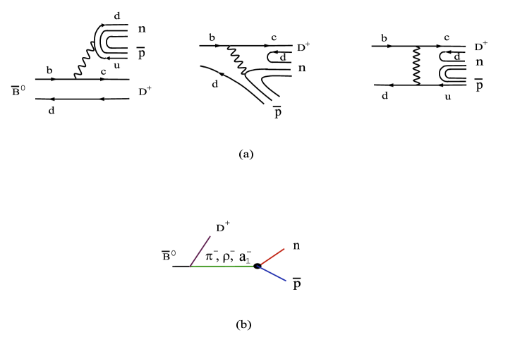
FIG. 1.: (a) Quark diagrams for $\overline{B}^{0}\to D^{+}n\bar{p}$ and (b) the pole diagram for the factorizable external $W$-emission.

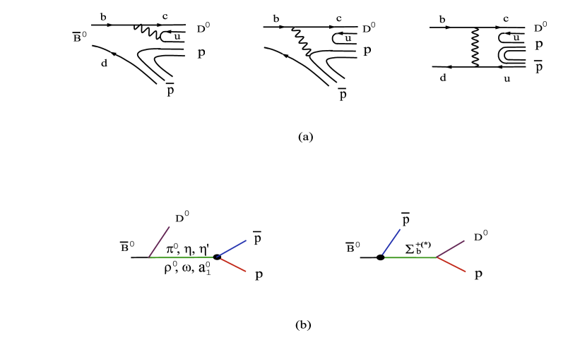
FIG. 2.: (a) Quark diagrams for $\overline{B}^{0}\to D^{0}p\bar{p}$ and (b) the pole diagrams for the factorizable internal $W$-emission.

Let us first focus on the decays $\overline{B}^{0}\to D^{+(*)}n\bar{p}$. To evaluate their factorizable amplitude, we need to know various haronic matrix elements. The one-body and two-body mesonic matrix elements are given by [11]

$$\langle P(q)|A_{\mu}|0\rangle = -if_{P}q_{\mu},\qquad\langle V(p,\varepsilon)|V_{\mu}|0\rangle=f_{V}m_{V}\varepsilon^{*}_{\mu},$$ (9)

$$\langle P(p)|V_{\mu}|B(p_{B})\rangle = \left(p_{B\mu}+p_{\mu}-{m_{B}^{2}-m_{P}^{2}\over q^{2}}\,q_{\mu}\right)F^{BP}_{1}(q^{2})+{m_{B}^{2}-m_{P}^{2}\over q^{2}}q_{\mu}\,F^{BP}_{0}(q^{2}),$$ (10)

$$\langle V(p,\varepsilon)|(V-A)_{\mu}|B(p_{B})\rangle = {2i\over m_{B}+m_{V}}\,\epsilon_{\mu\nu\alpha\beta}\varepsilon^{*\nu}p^{\alpha}p_{B}^{\beta}V^{BV}(q^{2})-\Bigg{\{}(m_{B}+m_{V})\varepsilon^{*}_{\mu}A^{BV}_{1}(q^{2})$$ (11)

$$- {\varepsilon^{*}\cdot p_{B}\over m_{B}+m_{V}}\,(p_{B}+p)_{\mu}A^{BV}_{2}(q^{2})$$ (12)

$$- 2m_{V}\,{\varepsilon^{*}\cdot p_{B}\over q^{2}}\,q_{\mu}\big{[}A^{BV}_{3}(q^{2})-A^{BV}_{0}(q^{2})\big{]}\Bigg{\}},$$ (13)

where $q=p_{B}-p$, $F_{1}(0)=F_{0}(0)$, $A_{3}(0)=A_{0}(0)$, and

$$A_{3}(q^{2})=\,{m_{B}+m_{V}\over 2m_{V}}\,A_{1}(q^{2})-{m_{B}-m_{V}\over 2m_{V}}\,A_{2}(q^{2}).$$ (14)

The two-body baryonic matrix element appearing in Eq. (5) can be parametrized as

$$\langle n(p_{n})\bar{p}(p_{\bar{p}})|(V-A)_{\mu}|0\rangle = \bar{u}_{n}(p_{n})\Bigg{\{}f_{1}^{np}(q^{2})\gamma_{\mu}+i{f_{2}^{np}(q^{2})\over 2m_{N}}\sigma_{\mu\nu}q^{\nu}+{f_{3}^{np}(q^{2})\over 2m_{N}}q_{\mu}$$ (16)

$$-\Big{[}g_{1}^{np}(q^{2})\gamma_{\mu}+i{g_{2}^{np}(q^{2})\over 2m_{N}}\sigma_{\mu\nu}q^{\nu}+{g_{3}^{np}(q^{2})\over 2m_{N}}q_{\mu}\Big{]}\gamma_{5}\Bigg{\}}v_{\bar{p}}(p_{\bar{p}}),$$

with $q=p_{p}+p_{\bar{p}}$. Among the six baryonic form factors, the vector form factor $f_{3}(q^{2})$ vanishes because of conservation of vector current (CVC), while the absence of the second-class current implies $g_{2}(q^{2})=0$. Using CVC, the vector form factors $f_{1,2}(q^{2})$ can be related to the electromagnetic form factors of the nucleon defined by

$$\langle N(p_{1})\overline{N}(p_{2})|J_{\mu}^{\rm em}|0\rangle=\bar{u}_{N}(p_{1})\Big{[}F_{1}(q^{2})\gamma_{\mu}+i{F_{2}(q^{2})\over 2m_{N}}\sigma_{\mu\nu}q^{\nu}\Big{]}v_{\bar{N}}(p_{2}).$$ (17)

Specifically (see e.g. [10]),

$$f^{np}_{1,2}(t)=F_{1,2}^{p}(t)-F_{1,2}^{n}(t),$$ (18)

where $t=q^{2}$.

The experimental data of the nucleon’s e.m. form factors are customarily described in terms of the electric and magnetic Sachs form factors $G_{E}^{N}(t)$ and $G_{M}^{N}(t)$ which are related to $F_{1}^{N}$ and $F_{2}^{N}$ via

$$G_{E}^{p,n}(t)=F_{1}^{p,n}(t)+{t\over 4m_{N}^{2}}F_{2}^{p,n}(t),\qquad G_{M}^{p,n}(t)=F_{1}^{p,n}(t)+F_{2}^{p,n}(t).$$ (19)

A recent phenomenological fit to the experimental data of nucleon form factors has been carried out in [12] using the following parametrization:

$$|G_{M}^{p}(t)| = \left({x_{1}\over t^{2}}+{x_{2}\over t^{3}}+{x_{3}\over t^{4}}+{x_{4}\over t^{5}}+{x_{5}\over t^{6}}\right)\left[\ln{t\over Q_{0}^{2}}\right]^{-\gamma},$$ (20)

$$|G_{M}^{n}(t)| = \left({y_{1}\over t^{2}}+{y_{2}\over t^{3}}\right)\left[\ln{t\over Q_{0}^{2}}\right]^{-\gamma},$$ (21)

where $Q_{0}=\Lambda_{\rm QCD}\approx$ 300 MeV and $\gamma=2+{4\over 3\beta}=2.148$ . We will follow [13] to use the best fit values

$$x_{1}=420.96\,{\rm GeV}^{4},\qquad x_{2}=-10485.50\,{\rm GeV}^{6},\qquad x_{3}=106390.97\,{\rm GeV}^{8},$$ (22)

$$x_{4}=-433916.61\,{\rm GeV}^{10},\qquad x_{5}=613780.15\,{\rm GeV}^{12},$$ (23)

and

$$y_{1}=236.69\,{\rm GeV}^{4},\qquad\quad y_{2}=-579.51\,{\rm GeV}^{6},$$ (24)

extracted from the neutron data under the assumption $|G_{E}^{n}|=|G_{M}^{n}|$. Note that the form factors given by Eq. (20) do satisfy the constraint from perturbative QCD in the limit of large $t$ [12]. Also as stressed in [12], time-like magnetic form factors are expected to behave like space-like magnetic form factors, i.e. real and positive for the proton, but negative for the neutron.

In terms of the nucleon magnetic and electric form factors, the weak form factors read

$$f^{np}_{1}(t) = {{t\over 4m_{N}^{2}}G_{M}^{p}(t)-G_{E}^{p}(t)\over t/(4m_{N}^{2})-1}-{{t\over 4m_{N}^{2}}G_{M}^{n}(t)-G_{E}^{n}(t)\over t/(4m_{N}^{2})-1},$$ (25)

$$f^{np}_{2}(t) = -{G_{M}^{p}(t)-G_{E}^{p}(t)\over t/(4m_{N}^{2})-1}+{G_{M}^{n}(t)-G_{E}^{n}(t)\over t/(4m_{N}^{2})-1}.$$ (26)

According to perturbative QCD, the weak form factors in the large $t$ limit have the asymptotic expressions [14]

$$f^{np}_{1}(t)\to G_{M}^{p}(t)-G_{M}^{n}(t),\qquad g^{np}_{1}(t)\to{5\over 3}G_{M}^{p}(t)+G_{M}^{n}(t).$$ (27)

It is easily seen that this is consistent with the large $t$ behavior of $f_{1}^{np}$ given by Eq. (25).

For the axial form factor $g_{1}(t)$, we shall follow [15] to assume that it has a similar expression as $G_{M}^{n}(t)$

$$g_{1}^{np}(t)=\left({d_{1}\over t^{2}}+{d_{2}\over t^{3}}\right)\left[\ln{t\over Q_{0}^{2}}\right]^{-\gamma},$$ (28)

where the coefficient $d_{1}$ is related to $x_{1}$ and $y_{1}$ by considering the asymptotic behavior of Sachs form factors $G_{M}^{p}$ and $G_{M}^{n}$ [see Eq. (20)]

$$d_{1}={5\over 3}x_{1}-y_{1}.$$ (29)

As shown in [10], the induced pseudoscalar form factor $g_{3}$ corresponds to a pion pole contribution to the $n\bar{p}$ axial matrix element and it has the form

$$g_{3}^{np}(t)=-{4m_{N}^{2}\over t-m_{\pi}^{2}}g_{1}^{np}(t).$$ (30)

III Color-suppressed $\overline{B}^{0}\to D^{(*)0}{p\bar{p}}$

We next turn to the color-suppressed modes $\overline{B}^{0}\to D^{(*)0}p\bar{p}$ and assume that the main contributions arise from the factorizable internal $W$-emission diagram [see Fig. 2(a)]. There are two corresponding pole diagrams as depicted in Fig. 2(b): one with bottom baryon poles $\Sigma_{b}({1\over 2}^{+})$ and $\Sigma_{b}^{*}({1\over 2}^{-})$, and the other with meson poles. The low-lying meson intermediate states are: $\pi^{0},\eta,\eta^{\prime}$, $\rho^{0},\omega$, and $a_{1}^{0}$ and possibly $f_{1}(1285)$ and $f_{1}(1420)$.

A Meson pole contributions

The meson pole contribution from Fig. 2 (b) is

$$A(\overline{B}^{0}\to D^{0}p\bar{p})_{\cal M} = {G_{F}\over\sqrt{2}}V_{ud}^{*}V_{cb}\,a_{2}\langle D^{0}|(\bar{c}u)|0\rangle\Bigg{\{}-\Big{[}\langle\pi^{0}|(\bar{d}b)|\overline{B}^{0}\rangle{i\over q^{2}-m_{\pi}^{2}}g_{\pi NN}$$ (31)

$$+ \langle\eta|(\bar{d}b)|\overline{B}^{0}\rangle{i\over q^{2}-m_{\eta}^{2}}g_{\eta NN}+\langle\eta^{\prime}|(\bar{d}b)|\overline{B}^{0}\rangle{i\over q^{2}-m_{\eta^{\prime}}^{2}}g_{\eta^{\prime}NN}\Big{]}\bar{u}_{p}\gamma_{5}v_{\bar{p}}$$ (32)

$$+ \langle\rho^{0}|(\bar{d}b)|\overline{B}^{0}\rangle{i\over q^{2}-m_{\rho}^{2}}\,\bar{u}_{p}\,\varepsilon_{\rho}^{\nu}\left(g_{1}^{\rho NN}\gamma_{\nu}+i{g_{2}^{\rho NN}\over 2m_{N}}\sigma_{\nu\lambda}q^{\lambda}\right)v_{\bar{p}}$$ (33)

$$+ \langle\omega|(\bar{d}b)|\overline{B}^{0}\rangle{i\over q^{2}-m_{\omega}^{2}}\,\bar{u}_{p}\,\varepsilon_{\omega}^{\nu}\left(g_{1}^{\omega NN}\gamma_{\nu}+i{g_{2}^{\omega NN}\over 2m_{N}}\sigma_{\nu\lambda}q^{\lambda}\right)v_{\bar{p}}$$ (34)

$$+ \langle a^{0}_{1}|(\bar{d}b)|\overline{B}^{0}\rangle{i\over q^{2}-m_{a_{1}}^{2}}\,g_{1}^{a_{1}NN}\bar{u}_{p}\,\varepsilon\!\!\!/_{a_{1}}\gamma_{5}v_{\bar{p}}\Bigg{\}},$$ (35)

where $q=p_{B}-p_{D}=p_{p}+p_{\bar{p}}$. For simplicity, we have concentrated on the low-lying poles and neglected those contributions from the higher axial vector meson states such as $f_{1}(1285)$ and $f_{1}(1420)$. As we shall see, the vector and tensor coupling constants $g_{1}^{\rho NN}$ and $g_{2}^{\rho NN}$ are related to the vector form factors $f_{1}^{np}$ and $f_{2}^{np}$ respectively, while $g_{1}^{a_{1}NN}$ and $g_{\pi NN}$ are connected to the axial-vector form factors $g_{1}^{np}$ and $g_{3}^{np}$ respectively.

After some manipulation we obtain

$$A(\overline{B}^{0}\to D^{0}p\bar{p})_{\cal M} = -{G_{F}\over\sqrt{2}}V_{ud}^{*}V_{cb}\,f_{D}a_{2}\Bigg{\{}\Big{[}{1\over\sqrt{2}}(m_{B}^{2}-m_{\pi}^{2})F_{0}^{B\pi}(m_{D}^{2}){g_{\pi NN}\over q^{2}-m_{\pi}^{2}}$$ (36)

$$+ (m_{B}^{2}-m_{\eta}^{2})F_{0}^{B\eta}(m_{D}^{2}){g_{\eta NN}\over q^{2}-m_{\eta}^{2}}+(m_{B}^{2}-m_{\eta^{\prime}}^{2})F_{0}^{B\eta^{\prime}}(m_{D}^{2}){g_{\eta^{\prime}NN}\over q^{2}-m_{\eta^{\prime}}^{2}}\Big{]}\bar{u}_{p}\gamma_{5}v_{\bar{p}}$$ (37)

$$+ {\sqrt{2}m_{\rho}\over q^{2}-m_{\rho}^{2}}A_{0}^{B\rho}(m_{D}^{2})\bar{u}_{p}\Big{[}-(g_{1}^{\rho NN}+g_{2}^{\rho NN})p\!\!\!/_{B}+{g_{2}^{\rho NN}\over 2m_{N}}(p_{p}-p_{\bar{p}})\cdot p_{B}\Big{]}v_{\bar{p}}$$ (38)

$$+ {2m_{\omega}\over q^{2}-m_{\omega}^{2}}A_{0}^{B\omega}(m_{D}^{2})\bar{u}_{p}\Big{[}-(g_{1}^{\omega NN}+g_{2}^{\omega NN})p\!\!\!/_{B}+{g_{2}^{\omega NN}\over 2m_{N}}(p_{p}-p_{\bar{p}})\cdot p_{B}\Big{]}v_{\bar{p}}$$ (39)

$$+ {\sqrt{2}m_{a_{1}}\over q^{2}-m_{a_{1}}^{2}}V_{0}^{Ba_{1}}(m_{D}^{2})g_{1}^{a_{1}NN}\bar{u}_{p}\Big{[}-p\!\!\!/_{B}+{p_{B}\cdot q\,q\!\!\!/\over m_{a_{1}}^{2}}\Big{]}\gamma_{5}v_{\bar{p}}\Bigg{\}},$$ (40)

where we have applied the relations $\bar{u}_{p}q\!\!\!/v_{\bar{p}}=0$, $(p_{p}-p_{\bar{p}})\cdot q=0$ and employed the form factors defined by

$$\langle a_{1}^{-}(p_{a_{1}})|(\bar{u}b)_{{}_{V-A}}|\overline{B}^{0}(p_{B})\rangle = {2i\over m_{B}+m_{a_{1}}}\epsilon_{\mu\nu\alpha\beta}\varepsilon^{*\nu}p^{\alpha}_{a_{1}}p^{\beta}_{B}A^{Ba_{1}}(q^{2})$$ (41)

$$- \Bigg{\{}(m_{B}+m_{a_{1}})\varepsilon^{*}_{\mu}V_{1}^{Ba_{1}}(q^{2})-{\varepsilon^{*}\cdot p_{B}\over m_{B}+m_{a_{1}}}(p_{B}+p_{a_{1}})_{\mu}V_{2}^{B\rho}(q^{2})$$ (42)

$$- 2m_{a_{1}}{\varepsilon^{*}\cdot p_{B}\over q^{2}}q_{\mu}\left[V_{3}^{Ba_{1}}(q^{2})-V_{0}^{Ba_{1}}(q^{2})\right]\Bigg{\}},$$ (43)

with

$$V_{3}(q^{2})=\,{m_{B}+m_{V}\over 2m_{V}}\,V_{1}(q^{2})-{m_{B}-m_{V}\over 2m_{V}}\,V_{2}(q^{2}),$$ (44)

and $V_{3}(0)=V_{0}(0)$. Note that the pion in the form factor $F_{0}^{B\pi}$ is referred to the charged one, so are the form factors $A_{0}^{B\rho}$ and $V_{0}^{Ba_{1}}$.

Likewise, the meson pole contribution to $\overline{B}^{0}\to D^{*0}p\bar{p}$ reads

$$A(\overline{B}^{0}\to D^{*0}p\bar{p})_{\cal M} = {G_{F}\over\sqrt{2}}V_{ud}^{*}V_{cb}\,a_{2}\,f_{D^{*}}m_{D^{*}}\Bigg{\{}\Big{[}\sqrt{2}F_{1}^{B\pi}(m_{D^{*}}^{2}){g_{\pi NN}\over q^{2}-m_{\pi}^{2}}$$ (45)

$$+ 2F_{1}^{B\eta}(m_{D^{*}}^{2}){g_{\eta NN}\over q^{2}-m_{\eta}^{2}}+2F_{1}^{B\eta^{\prime}}(m_{D^{*}}^{2}){g_{\eta^{\prime}NN}\over q^{2}-m_{\eta^{\prime}}^{2}}\Big{]}(\varepsilon^{*}_{D^{*}}\cdot p_{B})\bar{u}_{p}\gamma_{5}v_{\bar{p}}$$ (46)

$$+ \langle\rho^{0}|\bar{d}\,\varepsilon\!\!\!/_{D^{*}}^{*}(1-\gamma_{5})b|\overline{B}^{0}\rangle{1\over q^{2}-m_{\rho}^{2}}\bar{u}_{p}\,\varepsilon_{\rho}^{\mu}(g_{1}^{\rho NN}\gamma_{\mu}+i{g_{2}^{\rho NN}\over 2m_{N}}\sigma_{\mu\nu}q^{\nu})v_{\bar{p}}$$ (47)

$$+ \langle\omega|\bar{d}\,\varepsilon\!\!\!/_{D^{*}}^{*}(1-\gamma_{5})b|\overline{B}^{0}\rangle{1\over q^{2}-m_{\omega}^{2}}\bar{u}_{p}\,\varepsilon_{\omega}^{\mu}(g_{1}^{\omega NN}\gamma_{\mu}+i{g_{2}^{\omega NN}\over 2m_{N}}\sigma_{\mu\nu}q^{\nu})v_{\bar{p}}$$ (48)

$$+ \langle a_{1}^{0}|\bar{d}\,\varepsilon\!\!\!/_{D^{*}}^{*}(1-\gamma_{5})b|\overline{B}^{0}\rangle{1\over q^{2}-m_{a_{1}}^{2}}\bar{u}_{p}(g_{1}^{a_{1}NN}\varepsilon\!\!\!/_{a_{1}}\gamma_{5})v_{\bar{p}}\Bigg{\}}.$$ (49)

B Baryon pole contributions

In addition to the aforementioned meson pole contributions, there also exist baryon pole diagrams, namely, the strong process $\overline{B}^{0}\to\Sigma_{b}^{+(*)}\bar{p}$ followed by the weak decay $\Sigma^{+(*)}_{b}\to D^{0}p$. Due to the large theoretical uncertainties with the ${1\over 2}^{-}$ state $\Sigma_{b}^{+*}$, we will focus on the ${1\over 2}^{+}$ intermediate state and its amplitude is given by

$$A(\overline{B}^{0}\to D^{0}p\bar{p})_{\cal B} = {G_{F}\over\sqrt{2}}V_{ud}^{*}V_{cb}f_{D}\,a_{2}\,g_{\Sigma_{b}^{+}\to B\bar{p}}\,{1\over(p_{p}+p_{D})^{2}-m_{\Sigma_{b}}^{2}}$$ (50)

$$\times \bar{u}_{p}\Big{\{}f_{1}^{\Sigma_{b}^{+}p}(m_{D}^{2})[2p_{D}\cdot p_{p}+p\!\!\!/_{D}(m_{\Sigma_{b}}-m_{p})]\gamma_{5}$$ (51)

$$+ g_{1}^{\Sigma_{b}^{+}p}(m_{D}^{2})[2p_{D}\cdot p_{p}-p\!\!\!/_{D}(m_{\Sigma_{b}}+m_{p})]\Big{\}}v_{\bar{p}},$$ (52)

where we have applied the factorization approximation to the weak decay $\Sigma_{b}^{+}\to D^{0}p$. Similarly, for $\overline{B}^{0}\to D^{*0}p\bar{p}$ we have

$$A(\overline{B}^{0}\to D^{*0}p\bar{p})_{\cal B} = {G_{F}\over\sqrt{2}}V_{cb}V_{ud}^{*}f_{D^{*}}m_{D^{*}}\,a_{2}\,g_{\Sigma_{b}^{+}\to B\bar{p}}\,{1\over(p_{p}+p_{D^{*}})^{2}-m_{\Sigma_{b}}^{2}}$$ (53)

$$\times \bar{u}_{p}\,\varepsilon^{*\mu}\Big{\{}f_{1}^{\Sigma_{b}^{+}p}(m_{D^{*}}^{2})[2p_{p\mu}+(m_{\Sigma_{b}}-m_{p})\gamma_{\mu}+\gamma_{\mu}p\!\!\!/_{D}]\gamma_{5}$$ (54)

$$+ g_{1}^{\Sigma_{b}^{+}p}(m_{D^{*}}^{2})[2p_{p\mu}-(m_{\Sigma_{b}}+m_{p})\gamma_{\mu}+\gamma_{\mu}p\!\!\!/_{D}]\Big{\}}v_{\bar{p}},$$ (55)

where $\varepsilon_{\mu}^{*}$ is the polarization vector of the $D^{*}$.

The baryon pole contribution is expected to be suppressed relative to the meson pole due to the smallness of the strong coupling of $\Sigma_{b}^{+}\to B^{0}\bar{p}$ [10].

IV Calculations and Results

To proceed numerical calculations we first need to know the relevant form factors, decay constants, strong couplings, and the parameters $a_{1}$, $a_{2}$, which will be discussed in more detail below.

A form factors and decay constants

For the mesonic form factors of $B\to P$ and $B\to V$ transitions we use the Melikhov-Stech (MS) model based on the constituent quark picture [16] and the Neubert-Rieckert-Stech-Xu (NRSX) model [17] which takes the Bauer-Stech-Wirbel (BSW) model [11] results for the form factors at zero momentum transfer but makes a different ansatz for their $q^{2}$ dependence, namely, a dipole behavior is assumed for the form factors $F_{1},~{}A_{0},~{}A_{2},~{}V$, motivated by heavy quark symmetry, and a monopole dependence for $F_{0},A_{1}$.

For $B\to a_{1}$ form factors, there are two existing calculations: one in a quark-meson model [18] and the other based on the QCD sum rule [19]. The results are quite different, for example, $V^{Ba_{1}}(0)$ computed in the quark-meson model, 1.20 , is larger than the sum-rule prediction, $-0.23\pm 0.05$ , by a factor of five. We shall see later that $\overline{B}^{0}\to D^{0}p\bar{p}$ is rather sensitive to the form factor $V^{Ba_{1}}_{0}$. It turns that in order to accommodate the measurement of this decay, this form factor should be around 0.86 which is between the above-mentioned model calculations. In the present paper we shall use the quark-meson model results for the $B\to a_{1}$ form factors except that the value of $V^{Ba_{1}}_{0}(0)$ is replaced by 0.85 rather than 1.20 .

To compute the form factors for $F_{0}^{B\eta}$ and $F_{0}^{B\eta^{\prime}}$, it is more natural to consider the flavor basis of $\eta_{q}$ and $\eta_{s}$ defined by

$$\eta_{q}={1\over\sqrt{2}}(u\bar{u}+d\bar{d}),\qquad\quad\eta_{s}=s\bar{s}.$$ (56)

The wave functions of the $\eta$ and $\eta^{\prime}$ are given by

$$\left(\matrix{\eta\cr\eta^{\prime}\cr}\right)=\left(\matrix{\cos\phi&-\sin\phi\cr\sin\phi&\cos\phi\cr}\right)\left(\matrix{\eta_{q}\cr\eta_{s}\cr}\right),$$ (57)

where $\phi=\theta+{\rm arctan}\sqrt{2}$, and $\theta$ is the $\eta\!-\!\eta^{\prime}$ mixing angle in the octet-singlet basis. The physical form factors then have the simple expressions:

$$F_{0,1}^{B\eta}={1\over\sqrt{2}}\cos\phi\,F_{0,1}^{B\eta_{u\bar{u}}},\qquad F_{0,1}^{B\eta^{\prime}}={1\over\sqrt{2}}\sin\phi\,F_{0,1}^{B\eta^{\prime}_{u\bar{u}}}.$$ (58)

Using $F_{0}^{B\eta_{u\bar{u}}}(0)=0.307$ and $F_{0}^{B\eta^{\prime}_{u\bar{u}}}(0)=0.254$ obtained from [11] and the mixing angle $\phi=39.3^{\circ}$ (or $\theta=-15.4^{\circ}$) [20] we find $F_{0}^{B\eta}(0)=0.168$ and $F_{0}^{B\eta^{\prime}}(0)=0.114$ in the BSW model and hence the NRSX model. For other form-factor models, we shall apply the relation based on the isospin-quartet symmetry

$$F_{0,1}^{B\eta_{u\bar{u}}}=F_{0,1}^{B\eta^{\prime}_{u\bar{u}}}=F_{0,1}^{B\pi}$$ (59)

and Eq. (58) to obtain the physical $B\to\eta$ and $B\to\eta^{\prime}$ transition form factors. For the MS model we obtain $F_{0}^{B\eta}(0)=0.141$ and $F_{0}^{B\eta^{\prime}}(0)=0.115$.

For the heavy-light baryonic form factors $f_{1}^{\Sigma_{b}^{+}p}$ and $g_{i}^{\Sigma_{b}^{+}p}$, we will follow [21] to apply the nonrelativistic quark model to evaluate the weak current-induced baryon form factors at zero recoil in the rest frame of the heavy parent baryon, where the quark model is most trustworthy. Following [22] we have

$$f_{1}^{\Sigma_{b}^{+}p}(q^{2}_{m})=1.703,\qquad\qquad g_{1}^{\Sigma_{b}^{+}p}(q^{2}_{m})=-0.166$$ (60)

at zero recoil $q_{m}^{2}=(m_{\Sigma_{b}}-m_{p})^{2}$. Since the calculation for the $q^{2}$ dependence of form factors is beyond the scope of the non-relativistic quark model, we will follow the conventional practice to assume a pole dominance for the form-factor $q^{2}$ behavior:

$$f(q^{2})=f(q^{2}_{m})\left({1-q^{2}_{m}/m^{2}_{V}\over 1-q^{2}/m_{V}^{2}}\right)^{n}\,,\qquad g(q^{2})=g(q^{2}_{m})\left({1-q^{2}_{m}/m^{2}_{A}\over 1-q^{2}/m_{A}^{2}}\right)^{n}\,,$$ (61)

where $m_{V}$ ($m_{A}$) is the pole mass of the vector (axial-vector) meson with the same quantum number as the current under consideration.

For the decay constants we use $f_{D}=200$ MeV, $f_{D^{*}}=230$ MeV and $f_{a_{1}}=205$ MeV.

B strong couplings

In order to compute the decay rate for $\overline{B}^{0}\to D^{(*)0}p\bar{p}$ we also need to know the strong couplings $g_{\pi NN},\,g_{1}^{\rho NN},\,g_{2}^{\rho NN}$ and $g_{1}^{a_{1}NN}$ and their $q^{2}$ dependence. To do this, let us consider the pole contributions to $\overline{B}^{0}\to D^{(*)+}n\bar{p}$. In the pole model description, the relevant intermediate states are $\pi^{-},~{}\rho^{-}$ and $a_{1}^{-}(1260)$ as shown in Fig. 1(b). The matrix element $\langle n\bar{p}|(V-A)_{\mu}|0\rangle$ then reads

$$\langle n\bar{p}|(V-A)_{\mu}|0\rangle_{\rm pole} = \bar{u}_{n}\Bigg{\{}{\sqrt{2}f_{\rho}m_{\rho}\over q^{2}-m_{\rho}^{2}}\left[g_{1}^{\rho NN}\gamma_{\mu}+i{g_{2}^{\rho NN}\over 2m_{N}}\sigma_{\mu\nu}q^{\nu}\right]$$ (62)

$$- {\sqrt{2}f_{a_{1}}m_{a_{1}}\over q^{2}-m_{a_{1}}^{2}}g_{1}^{a_{1}NN}\gamma_{\mu}\gamma_{5}-{\sqrt{2}f_{\pi}g_{\pi NN}\over q^{2}-m_{\pi}^{2}}q_{\mu}\gamma_{5}\Bigg{\}}v_{\bar{p}}.$$ (63)

Comparing this with Eq. (16) we see that the $\rho^{-}$ meson is responsible for the vector form factors $f_{1}$ and $f_{2}$, $a_{1}^{-}(1260)$ for $g_{1}$ and $g_{2}$, and $\pi^{-}$ for the induced pseudoscalar form factor $g_{3}$. More precisely,

$$g_{1}^{\rho NN}(q^{2}) = {q^{2}-m_{\rho}^{2}\over\sqrt{2}f_{\rho}m_{\rho}}\,f_{1}^{np}(q^{2}),\qquad\quad g_{2}^{\rho NN}(q^{2})={q^{2}-m_{\rho}^{2}\over\sqrt{2}f_{\rho}m_{\rho}}\,f_{2}^{np}(q^{2}),$$ (64)

$$g_{1}^{a_{1}NN}(q^{2}) = {q^{2}-m_{a_{1}}^{2}\over\sqrt{2}f_{a_{1}}m_{a_{1}}}\,g_{1}^{np}(q^{2}),\qquad\quad g_{\pi NN}(q^{2})={(q^{2}-m_{\pi}^{2})\over 2\sqrt{2}f_{\pi}m_{N}}\,g_{3}^{np}(q^{2}).$$ (65)

As for the vector and tensor couplings of the $\omega$ meson, a priori they are not necessarily related to those of the $\rho$ meson. For simplicity we shall assume that $g_{1,2}^{\omega NN}(q^{2})=g_{1,2}^{\rho NN}(q^{2})/\sqrt{2}$, noting that the $\rho$ meson here is referred to the charged one.

As for the strong $\eta$ and $\eta^{\prime}$ couplings with nucleons, we shall apply the ${}^{3}P_{0}$ quark-pair creation model [23, 24] to estimate its strength relative to the pion. This model in which the $q\bar{q}$ pair is created from the vacuum with vacuum quantum numbers ${}^{3}P_{0}$ implies

$${g_{\eta p\bar{p}}\over g_{\pi p\bar{p}}}={\langle\Phi_{p^{\uparrow}}(124)\Phi_{\eta}(35)|\Phi_{p^{\uparrow}}(123)\Phi_{\rm vac}(45)\rangle\over\langle\Phi_{p^{\uparrow}}(124)\Phi_{\pi^{0}}(35)|\Phi_{p^{\uparrow}}(123)\Phi_{\rm vac}(45)\rangle},$$ (66)

where the $\Phi$’s are the spin-flavor wave functions and the vacuum wave function has the expression

$$\Phi_{\rm vac}={1\over\sqrt{3}}(u\bar{u}+d\bar{d}+s\bar{s})\otimes{1\over\sqrt{2}}(\uparrow\downarrow+\downarrow\uparrow).$$ (67)

Using the proton wave function

$$p^{\uparrow} = {1\over\sqrt{3}}[duu\chi_{s}+(12)+(13)],$$ (68)

with $abc\chi_{s}=(2a^{\downarrow}b^{\uparrow}c^{\uparrow}-a^{\uparrow}b^{\uparrow}c^{\downarrow}-a^{\uparrow}b^{\downarrow}c^{\uparrow})/\sqrt{6}$, the $\pi^{0}$ meson wave function

$$\Phi_{\pi^{0}}={1\over\sqrt{2}}(u\bar{u}-d\bar{d})\otimes{1\over\sqrt{2}}(\uparrow\downarrow-\downarrow\uparrow),$$ (69)

and the $\eta$ and $\eta^{\prime}$ flavor wave functions given by Eq. (57), we obtain

$${g_{\eta NN}\over g_{\pi NN}}={3\over 5}\cos\phi,\qquad\quad{g_{\eta^{\prime}NN}\over g_{\pi NN}}={3\over 5}\sin\phi.$$ (70)

Strictly speaking, the above relations hold only at low energies. But we shall assume their validity at arbitrary $q^{2}$.

As for the strong coupling $g_{\Sigma_{b}^{+}\to\overline{B}^{0}p}$, we use the experimental result for $B^{-}\to\Lambda_{c}\bar{p}\pi^{-}$ to fix the absolute coupling strength of $g_{\Lambda_{b}^{+}\to\overline{B}^{0}p}$ which is in turn related to $g_{\Sigma_{b}^{+}\to\overline{B}^{0}p}$ via the ${}^{3}P_{0}$ quark-pair-creation model [8]. It is found that $|g_{\Sigma_{b}^{+}\to\overline{B}^{0}p}|\sim 5$.

C $a_{1}$ and $a_{2}$

In the naive factorization approach, the parameters $a_{1}$ and $a_{2}$ are given by $a_{1,2}=c_{2,1}+c_{1,2}/N_{c}$, but this does not include nonfactorizable effects which are especially important for $a_{2}$. Phenomenologically, one can treat $a_{1,2}$ as free parameters and extract them from experiment. The experimental measurement of $B\to{J/\psi}K$ leads to $|a_{2}({J/\psi}K)|=0.26\pm 0.02$ [25]. This seems to be also supported by the study of $B\to D\pi$ decays: Assuming no relative phase between $a_{1}$ and $a_{2}$, the result $a_{2}\sim{\cal O}(0.20-0.30)$ [25, 26] is inferred from the data of $\overline{B}^{0}\to D^{(*)+}\pi^{-}$ and $B^{-}\to D^{(*)0}\pi^{-}$. However, the above value of $a_{2}$ leads to too small decay rates for $\overline{B}^{0}\to D^{(*)0}\pi^{0}$ when compared to recent measurements by Belle and CLEO [27]. In order to account for the observation, one needs a larger $a_{2}(D\pi)$ with a non-trivial phase relative to $a_{1}$ [28, 29, 30].

Using the measurements of CLEO and Belle for $\overline{B}^{0}\to D^{(*)0}\pi^{0}$ [27], the magnitudes of $a_{1}$ and $a_{2}$ and their relative phase are extracted in [29], as exhibited in Table I. We will use the values of $a_{1,2}(D\pi)$ to compute the decay rate for $\overline{B}^{0}\to D^{+}n\bar{p},D^{0}p\bar{p}$ and $a_{1,2}(D^{*}\pi)$ for $\overline{B}^{0}\to D^{*+}n\bar{p},D^{*0}p\bar{p}$.

TABLE I.: Extraction of the parameters $a_{1}$ and $a_{2}$ from the measured $B\to D^{(*)}\pi$ rates by assuming a negligible $W$-exchange contribution. Note that $a_{2}(D\pi)$ and $a_{2}(D^{*}\pi)$ should be multiplied by a factor of (200 MeV/$f_{D}$) and (230 MeV/$f_{D^{*}}$), respectively. This table is taken from [28].

Model	$|a_{1}(D\pi)|$	$|a_{2}(D\pi)|$	$a_{2}(D\pi)/a_{1}(D\pi)$	$|a_{1}(D^{*}\pi)|$	$|a_{2}(D^{*}\pi)|$	$a_{2}(D^{*}\pi)/a_{1}(D^{*}\pi)$
NRSX	$0.85\pm 0.06$	$0.40\pm 0.05$	$(0.47\pm 0.05)\,{\rm exp}(i59^{\circ})$	$0.94\pm 0.04$	$0.31\pm 0.04$	$(0.33\pm 0.04)\,{\rm exp}(i63^{\circ})$
MS	$0.88\pm 0.06$	$0.47\pm 0.06$	$(0.53\pm 0.06)\,{\rm exp}(i59^{\circ})$	$0.85\pm 0.03$	$0.39\pm 0.05$	$(0.46\pm 0.06)\,{\rm exp}(i63^{\circ})$

D Results

In principle, the unknown parameter $d_{2}$ appearing in the form factor $g_{1}^{np}(q^{2})$ [cf. Eq. (28)] can be fitted to the measured central value of the branching ratio for $\overline{B}^{0}\to D^{*+}n\bar{p}$ as it is theoretically much more clean. However, we find that the decay rate of $\overline{B}^{0}\to D^{0}p\bar{p}$ is dominated by the axial-vector meson poles and hence it is rather sensitive to $g^{np}_{1}(t)$ and hence $d_{2}$. Therefore, we instead fix it by fitting to the measured central value of ${\cal B}(\overline{B}^{0}\to D^{0}p\bar{p})=1.18\times 10^{-4}$. We obtain $d_{2}=-2070\,{\rm GeV}^{6}$ and $-2370\,{\rm GeV}^{6}$, respectively, in NRSX and MS form-factor models.

The total decay rate for the process $\overline{B}(p_{B})\to N(p_{1})+\overline{N}(p_{2})+D(p_{3})$ is computed by the formula

$$\Gamma={1\over(2\pi)^{3}}\,{1\over 32m_{B}^{3}}\int|A|^{2}dm_{12}^{2}dm_{23}^{2},$$ (71)

where $m_{ij}^{2}=(p_{i}+p_{j})^{2}$ with $p_{3}=p_{D}$. To compute the branching ratios, we use the $B$ meson lifetimes quoted in [31].

TABLE II.: Branching ratios (in units of $10^{-4}$) for charmful decays $\overline{B}^{0}\to D^{(*)+}n\bar{p}$ and $\overline{B}^{0}\to D^{(*)0}p\bar{p}$ calculated in the MS and NRSX form-factor models. The first (second) number in parentheses is the branching ratio due to the vector (axial-vector and pseudoscalar) current or intermediate vector (axial-vector) meson contributions.

Decay	MS	NRSX	Expt. [2, 4]
$\overline{B}^{0}\to D^{+}n\bar{p}$	$3.17~{}(3.04,0.12)$	$3.64~{}(3.47,0.16)$
$\overline{B}^{0}\to D^{*+}n\bar{p}$	$10.0~{}(9.54,0.49)$	$11.0~{}(10.2,0.76)$	$14.5^{+3.4}_{-3.0}\pm 2.7$
$\overline{B}^{0}\to D^{0}p\bar{p}$	$1.18~{}(0.15,1.03)$	$1.17~{}(0.11,1.06)$	$1.18\pm 0.15\pm 0.16$
$\overline{B}^{0}\to D^{*0}p\bar{p}$	$1.58~{}(1.42,0.17)$	$1.23~{}(1.12,0.11)$	$1.20^{+0.33}_{-0.29}\pm 0.21$

The results are shown in Table II. As stated before, we fit the unknown parameter $d_{2}$ to the measured branching ratio of $\overline{B}^{0}\to D^{0}p\bar{p}$ and then in turn predict other neutral baryonic $B$ modes. The baryon pole contributions to $D^{(*)0}p\bar{p}$ are found to be at most of order of $10^{-6}$ and hence they are negligible. It is clear from Table II that the predicted rates are consistent with experiment. We see that $\overline{B}^{0}\to D(D^{*})N\overline{N}$ are dominated by the vector current or by vector meson intermediate states, whereas $\overline{B}^{0}\to D^{0}p\bar{p}$ is dominated by the axial-vector intermediate state $a_{1}(1260)$. Note that the ratio $D^{*+}/D^{+}$ is of order 3, while $D^{*0}/D^{0}$ is close to unity.

In Fig. 3 we show the $n\bar{p}$ invariant mass distributions $d{\cal B}/dm_{n\bar{p}}$ of $\overline{B}^{0}\to D^{*+}n\bar{p}$ and $\overline{B}^{0}\to D^{+}n\bar{p}$, where $m_{n\bar{p}}$ is the invariant mass of the nucleon pair. Evidently, the spectrum peaks at $m_{p\bar{p}}\sim 2.1\,{\rm GeV}$, indicating a threshold enhancement for baryon production, that is, a recoil charmed meson is accompanied by a nucleon pair with low invariant mass. This effect is due to the suppression of the baryonic form factors at large $t$. Physically, this can be visualized that the quark and anti-quark forming a nucleon pair are moving collinearly and energetically, so that the invariant mass $m_{p\bar{p}}$ tends to be small and near threshold.

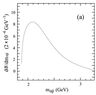
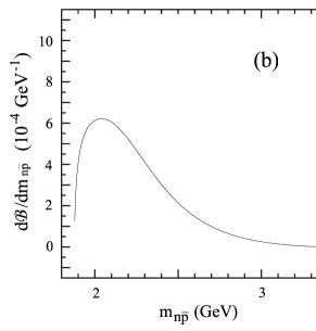
FIG. 3.: The $n\bar{p}$ invariant mass distribution $d{\cal B}/dm_{n\bar{p}}$ of (a) $\overline{B}^{0}\to D^{*+}n\bar{p}$ and (b) $\overline{B}^{0}\to D^{+}n\bar{p}$.

Also shown in Fig. 4 are the $p\bar{p}$ invariant mass distributions of $\overline{B}^{0}\to D^{*0}p\bar{p}$ and $\overline{B}^{0}\to D^{0}p\bar{p}$ calculated in the MS model. It is clear that the spectrum of $D^{*0}p\bar{p}$ is similar to that of $D^{(*)+}n\bar{p}$. As for the differential rate of $D^{0}p\bar{p}$, it has a hump around $m_{p\bar{p}}\sim 3.0$ GeV, which is caused by the mass term $q^{\mu}q^{\nu}/m_{a_{1}}^{2}$ in the propagator of the $a_{1}$ meson. We see that the predicted spectrum is consistent with experiment.

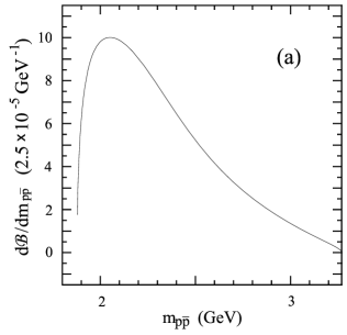
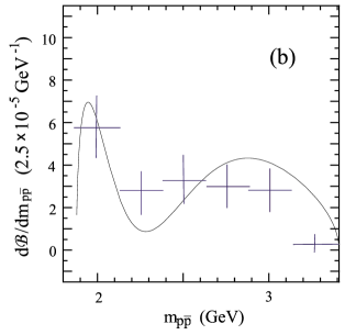
FIG. 4.: The $p\bar{p}$ invariant mass distribution $d{\cal B}/dm_{p\bar{p}}$ of (a) $\overline{B}^{0}\to D^{*0}p\bar{p}$ and (b) $\overline{B}^{0}\to D^{0}p\bar{p}$. The experimental data for the spectrum of $\overline{B}^{0}\to D^{0}p\bar{p}$ are taken from [3].

V Conclusions

We have studied the charmful three-body baryonic $B$ decays $\overline{B}\to D^{(*)}N\overline{N}$: the color-allowed modes $\overline{B}^{0}\to D^{(*)+}n\bar{p}$ and the color-suppressed ones $\overline{B}^{0}\to D^{(*)0}p\bar{p}$. While the $D^{*+}/D^{+}$ production ratio is predicted to be of order 3, it is found that $D^{0}p\bar{p}$ has a similar rate as $D^{*0}p\bar{p}$. It is pointed out that $\overline{B}^{0}\to D(D^{*})N\overline{N}$ are dominated by the nucleon vector current or by vector meson intermediate states, whereas $\overline{B}^{0}\to D^{0}p\bar{p}$ proceeds predominately via the axial-vector intermediate state $a_{1}(1260)$. The study of the $N\bar{N}$ invariant mass distribution in general indicates a threshold baryon pair production, that is, a recoil charmed meson accompanied by a low mass baryon pair except that the spectrum of $D^{0}p\bar{p}$ has a hump at large $p\bar{p}$ invariant mass $m_{p\bar{p}}\sim 3.0$ GeV. The presence of a hump in the $D^{0}p\bar{p}$ spectrum can be tested by the improved experiment in the future.

- [1]
- [2] CLEO Collaboration, S. Anderson et al., Phys. Rev. Lett. 86, 2732 (2001).
- [3] CLEO Collaboration, T.E. Coan et al., Phys. Rev. D59, 111101 (1999); Belle Collaboration, K. Abe et al., Phys. Rev. D65, 091103 (2002).
- [4] Belle Collaboration, K. Abe et al., hep-ex/0205083.
- [5] CLEO Collaboration, X. Fu et al., Phys. Rev. Lett. 79, 3125 (1997).
- [6] Belle Collaboration, K. Abe et al., BELLE-CONF-0238 (2002).
- [7] CLEO Collaboration, S.A. Dytman et al., hep-ex/0208006.
- [8] H.Y. Cheng and K.C. Yang, Phys. Rev. D65, 054028 (2002); ibid D65, 099901(E) (2002).
- [9] Belle Collaboration, K. Abe et al., Phys. Rev. Lett. 88, 181803 (2002).
- [10] H.Y. Cheng and K.C. Yang, Phys. Rev. D66, 014020 (2002).
- [11] M. Wirbel, B. Stech, and M. Bauer, Z. Phys. C29, 637 (1985); M. Bauer, B. Stech, and M. Wirbel, Z. Phys. C34, 103 (1987).
- [12] C.K. Chua, W.S. Hou, and S.Y. Tsai, Phys. Rev. D65, 034003 (2002).
- [13] C.K. Chua, W.S. Hou, and S.Y. Tsai, Phys. Lett. B528, 233 (2002).
- [14] S.J. Brodsky, G.P. Lapage, and S.A.A. Zaidi, Phys. Rev. D23, 1152 (1981).
- [15] C.K. Chua, W.S. Hou, and S.Y. Tsai, hep-ph/0204185.
- [16] D. Melikhov and B. Stech, Phys. Rev. D62, 014006 (2001).
- [17] M. Neubert, V. Rieckert, B. Stech, and Q.P. Xu, in Heavy Flavours, 1st edition, edited by A.J. Buras and M. Lindner (World Scientific, Singapore, 1992), p.286.
- [18] A. Deandrea, R. Gatto, G. Nardulli, and A.D. Polosa, Phys. Rev. D59, 074012 (1999).
- [19] T.M. Aliev and M. Savci, Phys. Lett. B456, 256 (1999).
- [20] T. Feldmann, P. Kroll, and B. Stech, Phys. Rev. D58, 114006 (1998); Phys. Lett. B449, 339 (1999).
- [21] H.Y. Cheng and B. Tseng, Phys. Rev. D53, 1457 (1996).
- [22] H.Y. Cheng, Phys. Rev. D56, 2799 (1997).
- [23] A. Le Yaouanc, L. Oliver, O. Péne, and J.-C. Raynal, Hadron Transitions in the Quark Model (Gordon and Breach Science Publishers, 1988).
- [24] M. Jarfi et al., Phys. Rev. D43, 1599 (1991); Phys. Lett. B237, 513 (1990).
- [25] H.Y. Cheng and K.C. Yang, Phys. Rev. D59, 092004 (1999).
- [26] M. Neubert and B. Stech, in Heavy Flavours, 2nd edition, ed. by A.J. Buras and M. Lindner (World Scientific, Singapore, 1998), p.294 [hep-ph/9705292].
- [27] Belle Collaboration, K. Abe et al., Phys. Rev. Lett. 88, 052002 (2002); CLEO Collaboration, T.E. Coan et al., Phys. Rev. Lett. 88, 062001 (2002).
- [28] Z.Z. Xing, hep-ph/0107257.
- [29] H.Y. Cheng, Phys. Rev. D65, 094012 (2002).
- [30] M. Neubert and A.A. Petrov, Phys. Lett. B519, 50 (2001).
- [31] Particle Data Group, K. Hagiwara et al., Phys. Rev. D66, 010001 (2002).