Abstract

Tools for calculating the Renormalization Group Equations for renormalizable and non-renormalizable operators in various theories are reviewed, which are essential for comparing experimental results with predictions from models beyond the Standard Model. Numerical examples for the running of the lepton mixing angles in models with non-degenerate see-saw scales are shown, in which the best-fit values of the experimentally favored LMA solution are produced from maximal or from vanishing solar neutrino mixing at the GUT scale.

1 Introduction

Models for neutrino masses typically operate at high energy scales, like the GUT scale. However from the experiments we obtain information about the low energy values of the parameters. To compare them, it is essential to evolve the parameters of the models from high to low energies. This is accomplished by the Renormalization Group Equations (RGE’s) for the operators of the theory. When the Standard Model (SM) or the MSSM is viewed as an effective field theory, Majorana masses for the neutrinos can be introduced via an effective operator of mass dimension 5, which couples 2 lepton and 2 Higgs doublets. The most promising scenarios for giving masses to neutrinos use the see-saw mechanism, which provides a convincing explanation for their smallness. It can be realized by a renormalizable theory with the particle content of the SM or the MSSM extended by 3 heavy neutrinos that are singlets under the SM gauge groups. The singlets typically have large explicit (Majorana) masses with a spectrum, which is non-degenerate in general. Due to this non-degeneracy one has to use several effective theories with the singlets partly integrated out, when studying the evolution of the effective mass matrix of the light neutrinos. We review the tools necessary to perform the Renormalization Group analysis of the neutrino mass parameters in various models. Numerical solutions to the RGE’s show that there can be large effects for the running of the lepton mixing angles, especially for the solar angle $\theta_{12}$. The currently favored LMA solution of the solar neutrino problem can e.g. be obtained in a natural way from bimaximal mixing [2] as well as from $\theta_{12}=\theta_{13}=0^{\circ}$, $\theta_{23}=45^{\circ}$ [3] at the GUT scale by renormalization group effects.

2 The Neutrino Mass Operator in the SM and in the MSSM

Let $\ell_{\mathrm{L}}^{f}$, $f\in\{1,2,3\}$, be the SU(2)_L-doublets of SM leptons and $\phi$ the Higgs doublet. The dimension 5 operator, which gives Majorana masses to the SM neutrinos after electroweak (EW) symmetry breaking (figure 1), is given by

$$\mathscr{L}_{\kappa}=\frac{1}{4}\kappa_{gf}\,\overline{\ell_{\mathrm{L}}^{\mathrm{C}}}^{g}_{c}\varepsilon^{cd}\phi_{d}\,\,\ell_{\mathrm{L}b}^{f}\varepsilon^{ba}\phi_{a}+\text{h.c.}\;.$$ (1)

$\kappa$ is symmetric under interchange of the generation indices $f$ and $g$, $\varepsilon$ is the totally antisymmetric tensor in 2 dimensions, and $\ell_{\mathrm{L}}^{\mathrm{C}}:=(\ell_{\mathrm{L}})^{\mathrm{C}}$ is the charge conjugate of the lepton doublet. $a,b,c,d\in\{1,2\}$ are SU(2) indices. The corresponding expression in the MSSM is the $F$-term of the part of the superpotential

$$\mathscr{W}_{\kappa}^{\mathrm{MSSM}}=-\frac{1}{4}{{\kappa}_{gf}}\,{\mathbb{l}^{g}_{c}}\varepsilon^{cd}{\mathbb{h}^{(2)}_{d}}\,\,\mathbb{l}_{b}^{f}\varepsilon^{ba}\mathbb{h}^{(2)}_{a}+\text{h.c.}\;,$$ (2)

where the chiral superfield $\mathbb{l}$ contains the lepton SU(2)_L-doublets and $\mathbb{h}^{(2)}$ contains the Higgs doublet with weak hypercharge $+\tfrac{1}{2}$.

$\vbox{\hbox{\includegraphics[scale={1}]{EFTDiagram2.eps}}}\xrightarrow[\mbox{{\small breaking}}]{\mbox{{\small EW symmetry}}}\vbox{\hbox{\includegraphics[scale={1}]{EFTDiagram1.eps}}}$

Figure 1: Vertex from the dimension 5 operator, which yields a Majorana mass matrix for the light neutrinos.

3 Calculating $\boldsymbol{\beta}$-Functions from Counterterms in MS-like Schemes

We are interested in the $\beta$-function $\beta_{Q}:=\mu\frac{\mathrm{d}Q}{\mathrm{d}\mu}$ for a quantity $Q$ in an MS-like renormalization scheme. In general, the bare and the renormalized quantity are related by

$$Q_{\mathrm{B}} = \left(\prod_{i\in I}Z_{\phi_{i}}^{n_{i}}\right)\,[Q+\delta Q]\mu^{D_{Q}\epsilon}\,\left(\prod_{j\in J}Z_{\phi_{j}}^{n_{j}}\right)\;,$$ (3)

where $I=\{1,\dots,M\}$, $J=\{M+1,\dots,N\}$, $D_{Q}$ is related to the mass dimension of $Q$, $\mu$ is the renormalization scale and $\epsilon:=4-d$ stems from dimensional regularization. $\delta Q$, which corresponds to the counterterm for $Q$, and the wavefunction renormalization constants $Z$ depend on $Q$ and some additional variables $\{V_{A}\}$. From equation (3), we obtain [4]

$$\beta_{Q} = \left[\sum_{A}D_{V_{A}}\Braket{\frac{\mathrm{d}\delta Q_{,1}}{\mathrm{d}V_{A}}}{V_{A}}-D_{Q}\,\delta Q_{,1}\right]+Q\cdot\sum_{j\in J}n_{j}\left[\sum_{A}D_{V_{A}}\,\Braket{\frac{\mathrm{d}Z_{\phi_{j},1}}{\mathrm{d}V_{A}}}{V_{A}}\right]$$ (4)

$$+\sum_{i\in I}n_{i}\left[\sum_{A}D_{V_{A}}\,\Braket{\frac{\mathrm{d}Z_{\phi_{i},1}}{\mathrm{d}V_{A}}}{V_{A}}\right]\cdot Q\;,$$

with $\Braket{\frac{\mathrm{d}F}{\mathrm{d}x}}{y}$ defined as $\frac{\mathrm{d}F}{\mathrm{d}x}y$ for scalars, $\sum_{n}\frac{\mathrm{d}F}{\mathrm{d}x_{n}}y_{n}$ for vectors, $\sum_{m,n}\frac{\mathrm{d}F}{\mathrm{d}x_{mn}}y_{mn}$ for matrices and analog for arbitrary tensors $x,y$. The formula (4) can be used for any tensorial quantity $Q$. Due to the general form of the counterterm in equation (3), it can also be used for non-multiplicative renormalization.

4 The $\boldsymbol{\beta}$-Function for the Neutrino Mass Operator in the SM and in 2HDM’s

Calculating the counterterm for the neutrino mass operator and the wavefunction renormalization constants in the SM, we obtain for the $\beta$-function of the neutrino mass operator from equation (4) [4]

$$16\pi^{2}\beta_{\kappa} = -\frac{3}{2}\left[\kappa\left(Y_{e}^{\dagger}Y_{e}\right)+\left(Y_{e}^{\dagger}Y_{e}\right)^{T}\kappa\right]+$$ (5)

$$+\lambda\kappa-3g_{2}^{2}\kappa+2\,\text{Tr}\left(3Y_{u}^{\dagger}Y_{u}+3Y_{d}^{\dagger}Y_{d}+Y_{e}^{\dagger}Y_{e}\right)\kappa\;.$$

$g_{2}$ is the SU(2) gauge coupling constant, $Y_{u}$ and $Y_{d}$ are the Yukawa matrices for the up and the down quarks, $Y_{e}$ is the Yukawa matrix for the charged leptons and $\lambda$ is the Higgs self-coupling. Compared to earlier results [5, 6], in [4] we find a coefficient $-\tfrac{3}{2}$ instead of $-\tfrac{1}{2}$ in front of the non-diagonal term $\kappa(Y_{e}^{\dagger}Y_{e})+(Y_{e}^{\dagger}Y_{e})^{T}\kappa$ (see figure 2), which is essential for the running of the lepton mixing angles. Similar corrections have also been made in the RGE’s for the neutrino mass operators in Two Higgs Doublet Models (2HDM’s) [7].

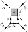
(a)

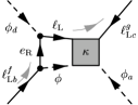
(b)

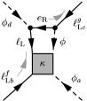
(c)

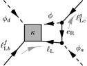
(d)

Figure 2: Diagrams for the 1-loop vertex renormalization of the neutrino mass operator in the SM, which yield contributions to the $\beta$-function with a non-trivial flavour structure. The gray arrow indicates the fermion flow as defined in [8].

5 Supergraph Construction Kit for 2-Loop $\boldsymbol{\beta}$-Functions in the MSSM

The calculation of $\beta$-functions is simplified considerably in supersymmetric (SUSY) theories, since due to the non-renormalization theorem [9, 10] only wavefunction renormalization has to be considered for operators of the superpotential. However, in a component field description, no use can be made of the theorem with respect to gauge loop corrections since it is no longer manifest when a supergauge, as for example Wess-Zumino-gauge, has been fixed. The supergraph technique [11, 12, 13, 14], on the other hand, allows to use the non-renormalization theorem since SUSY is kept manifest. It can thus be used to calculate $\beta$-functions in supersymmetric theories for operators of the superpotential from the wavefunction renormalization constants. These operators may be non-renormalizable since for the latter the non-renormalization theorem holds as well [15] and they do not affect the wavefunction renormalization constants in leading order in an effective field theory expansion. For the wavefunction renormalization constants, general formulae exist in the literature. Thus one can formulate a construction kit for calculating 2-loop beta functions in $N\!=\!1$ supersymmetric theories, which can be applied to renormalizable and non-renormalizable operators of the superpotential [16]. We applied it to calculate the 2-loop beta functions for the lowest-dimensional effective neutrino mass operator in the MSSM and for the Yukawa couplings (including $Y_{\nu}$) in the MSSM extended by singlet superfields and the Majorana mass matrix $M$ for the latter.

6 The 2-Loop $\boldsymbol{\beta}$-Function for the Neutrino Mass Operator in the MSSM

The calculation of the 1-loop part of the RGE for the neutrino mass operator in the MSSM yields

$$(4\pi)^{2}{\beta^{(1)}_{\kappa}}^{\mathrm{MSSM}}=(Y_{e}^{\dagger}Y_{e})^{T}{\kappa}+{\kappa}(Y_{e}^{\dagger}Y_{e})+6\,\text{Tr}(Y_{u}^{\dagger}Y_{u})\,{\kappa}-2g_{1}^{2}{\kappa}-6g_{2}^{2}{\kappa}\;,$$ (6)

confirming the existing MSSM result [5, 6]. Using the construction kit, from the supergraph diagrams shown in figure 3, for the 2-loop part we obtain [16]

$$(4\pi)^{4}\,{\beta^{(2)}_{\kappa}}^{\mathrm{MSSM}}=\left[-6\,\mbox{Tr}\,(Y_{u}^{\dagger}Y_{d}Y_{d}^{\dagger}Y_{u})-18\,\mbox{Tr}\,(Y_{u}^{\dagger}Y_{u}Y_{u}^{\dagger}Y_{u})+\frac{8}{5}\,g_{1}^{2}\,\mbox{Tr}\,(Y_{u}^{\dagger}Y_{u})\right.$$ (7)

$$+\left.32\,g_{3}^{2}\,\mbox{Tr}\,(Y_{u}^{\dagger}Y_{u})+\frac{207}{25}\,\,g_{1}^{4}+\frac{18}{5}\,g_{1}^{2}\,g_{2}^{2}+15\,g_{2}^{4}\right]\,\kappa$$

$$-\left[2\,(Y_{e}^{\dagger}Y_{e}Y_{e}^{\dagger}Y_{e})^{T}-\left(\frac{6}{5}\,g_{1}^{2}-\mbox{Tr}\,(Y_{e}Y_{e}^{\dagger})-3\,\mbox{Tr}\,(Y_{d}Y_{d}^{\dagger})\right)\,(Y_{e}^{\dagger}Y_{e})^{T}\right]\,\kappa$$

$$-\,\kappa\,\left[2\,Y_{e}^{\dagger}Y_{e}Y_{e}^{\dagger}Y_{e}-\left(\frac{6}{5}\,g_{1}^{2}-\mbox{Tr}\,(Y_{e}Y_{e}^{\dagger})-3\,\mbox{Tr}\,(Y_{d}Y_{d}^{\dagger})\right)\,Y_{e}^{\dagger}Y_{e}\right]\;.$$

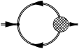
(a)

(b)

(c)

(d)

(e)

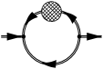
(f)

(g)

(h)

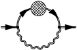
(i)

Figure 3: 2-loop supergraphs, which contribute to the $\overline{\bbPhi}\bbPhi$ propagator. Chiral superfields are represented as straight double lines while vector-superfields are indicated by wiggly double lines. A blob denotes the relevant one-particle irreducible graph including any 1-loop counterterm that may be required [17].

7 Generating the LMA solution by RG Running of the Lepton Mixing Angles

To study the RG running of the lepton mixing angles and neutrino masses, all parameters of the theory have to be evolved from the GUT scale to the EW scale. Starting at the GUT scale, the strategy is to successively solve the systems of coupled differential equations of the form

$$\mu\frac{\mathrm{d}}{\mathrm{d}\mu}\accentset{(n)}{X}_{i}=\accentset{(n)}{\beta}_{{X}_{i}}\raise 3.0pt\hbox{$\displaystyle\Bigl{(}$}\raise 3.0pt\hbox{$\displaystyle\Bigl{\{}$}\accentset{(n)}{X}_{j}\raise 3.0pt\hbox{$\displaystyle\Bigl{\}}$}\raise 3.0pt\hbox{$\displaystyle\Bigl{)}$}$$ (8)

for all the parameters $\accentset{(n)}{X}_{i}\in\raise 3.0pt\hbox{$\displaystyle\bigl{\{}$}\accentset{(n)}{\kappa},\accentset{(n)}{Y_{\nu}},\accentset{(n)}{M},\dots\raise 3.0pt\hbox{$\displaystyle\bigr{\}}$}$ of the theory. The parameters defined in the energy ranges corresponding to the various effective theories are marked by $(n)$. The derivation of the RGE’s for the theories in the ranges between the see-saw scales, where the heavy singles are partly integrated out, and the method for dealing with these effective theories are given in [18].

The LMA solution of the solar neutrino problem with a large but non-maximal value of the solar mixing angle $\theta_{12}$ is strongly favored by the experiments. The best-fit values are $\approx 33^{\circ}$ for $\theta_{12}$ [19, 20, 21, 22], $45^{\circ}$ for $\theta_{23}$ [23], while for $\theta_{13}$ at $2\sigma$ there is an upper bound of $\approx 9^{\circ}$ [24]. For model builders, especially the desired solar angle is difficult to achieve. This raises the question, whether the LMA solution might be reached by RG evolution if one starts with bimaximal lepton mixing or with vanishing solar mixing (and $\theta_{13}=0^{\circ},\theta_{23}=45^{\circ}$) at the GUT scale. Figure 4 shows examples for the RG evolution of the lepton mixing angles, where this has been accomplished [2, 3].

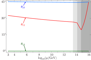
(a)

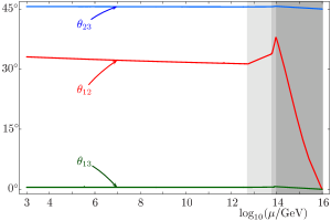
(b)

Figure 4: Examples for the RG evolution of the lepton mixing angles from the GUT scale to the SUSY-breaking scale (taken to be $\approx 1$ TeV) in the MSSM extended by 3 heavy singlets (right-handed neutrinos). We assumed zero CP phases and positive mass eigenvalues for the neutrinos. The best-fit values for the mixing angles of the LMA solution can be obtained from bimaximal lepton mixing [2] (figure 4(a)) as well as from vanishing solar mixing angle at the GUT scale [3] (figure 4(b)). The kinks in the plots correspond to the mass thresholds at the see-saw scales, where the heavy singlets are successively integrated out. The grey-shaded regions mark the various effective theories between the see-saw scales.

8 Conclusions

The Renormalization Group analysis of the neutrino mass parameters and lepton mixing angles provides a crucial tool towards understanding the physics at high energy scales. The necessary RGE’s in see-saw scenarios for neutrino masses have been derived for the various effective theories between the GUT scale and the low scale. For the energy ranges between the see-saw scales, the RGE’s have been derived in [18]. The RGE’s in the MSSM are known up to the 2-loop level [16]. This accuracy may be needed for the neutrino sector since due to the absence of hadronic uncertainties, high precision measurements of the neutrino parameters may be achieved in future experiments. The RGE for the neutrino mass operator at the 1-loop level has been derived in [5, 6, 4] for the SM, in [6, 7] for Two Higgs Doublet Models and in [5, 6, 7] for the MSSM. Numerical calculations show that large RG evolution of the lepton mixing angles can particularly take place in the energy ranges between and above the see-saw scales. The best-fit values for the mixing angles of the LMA solution can be obtained from bimaximal lepton mixing [2] as well as from single maximal mixing with a vanishing solar mixing angle [3] at the GUT scale.

References

- [1]
- [2] S. Antusch, J. Kersten, M. Lindner and M. Ratz, hep-ph/0206078.
- [3] S. Antusch and M. Ratz, hep-ph/0208136.
- [4] S. Antusch, M. Drees, J. Kersten, M. Lindner, M. Ratz, Phys. Lett. B519 (2001), 238–242.
- [5] P. H. Chankowski and Z. Pluciennik, Phys. Lett. B316 (1993), 312.
- [6] K. S. Babu, C. N. Leung and J. Pantaleone, Phys. Lett. B319 (1993), 191.
- [7] S. Antusch, M. Drees, J. Kersten, M. Lindner, M. Ratz, Phys. Lett. B525 (2002), 130.
- [8] A. Denner, H. Eck, O. Hahn, J. Küblbeck, Nucl. Phys. B387 (1992), 467.
- [9] J. Wess and B. Zumino, Phys. Lett. B49 (1974), 52.
- [10] J. Iliopoulos and B. Zumino, Nucl. Phys. B76 (1974), 310.
- [11] R. Delbourgo, Nuovo Cim. A25 (1975), 646.
- [12] A. Salam and J. Strathdee, Nucl. Phys. B86 (1975), 142–152.
- [13] K. Fujikawa and W. Lang, Nucl. Phys. B88 (1975), 61.
- [14] M. T. Grisaru, W. Siegel and M. Rocek, Nucl. Phys. B159 (1979), 429.
- [15] S. Weinberg, Phys. Rev. Lett. 80 (1998), 3702–3705.
- [16] S. Antusch and M. Ratz, JHEP 0207 (2002), 059.
- [17] P. West, Phys. Lett. B137 (1984), 371.
- [18] S. Antusch, J. Kersten, M. Lindner and M. Ratz, Phys. Lett. B538 (2002), 87–95.
- [19] V. Barger, D. Marfatia, K. Whisnant, and B. P. Wood, Phys. Lett. B537 (2002), 179–186.
- [20] A. Bandyopadhyay, S. Choubey, S. Goswami and D. P. Roy, Phys. Lett. B540 (2002), 14.
- [21] J. N. Bahcall, M. C. Gonzalez-Garcia and C. Peña-Garay, JHEP 0207 (2002), 054.
- [22] P. C. de Holanda and A. Yu. Smirnov, hep-ph/0205241.
- [23] T. Toshito et al. [Super-Kamiokande Collaboration], hep-ex/0105023.
- [24] M. Apollonio et al. [CHOOZ Collaboration], Phys. Lett. B466 (1999), 415.
- [25]
- [26]