A new Supersymmetric $SU(3)_{L}\otimes U(1)_{X}$ gauge model

Abstract

We present a new supersymmetric version of the $SU(3)\otimes U(1)$ gauge model using a more economic content of particles. The model has a smaller set of free parameters than other possibilities considered before. The MSSM can be seen as an effective theory of this larger symmetry. We find that the upper bound of the ligthest CP-even Higgs boson can be moved up to 140 GeV.

1 Introduction

In recent years it has been established with great precision that interactions of the gauge bosons with the fermions are well described by the Standard Model (SM) [1]. However, some sectors of the SM have not been tested yet, this is the case of the Higgs sector, responsible for the symmetry breaking. Despite all its success, the SM still has many unanswered questions. Among the various candidates to physics beyond the SM, supersymmetric theories play a special role. Although there is not yet direct experimental evidence of Supersymmetry (SUSY), there are many theoretical arguments indicating that SUSY might be of relevance for physics beyond the SM. The most popular version, of course, is the supersymmetric version of the SM, usually called MSSM.

Another approach to solve the fundamental problems of the SM is considering a larger symmetry which is broken to the SM symmetry using Higgs mechanisms. Among these cases $SU(3)_{L}\otimes U(1)_{X}$ as a local gauge theory has been studied previously by many authors who have explored different spectra of fermions and Higgs bosons [2]. There are many considerations about this model but the most studied motivations of this large symmetry are the possibility to give mass to the neutrino sector [3], anomaly cancellations in a natural way in the 3-family version of the model, and an interpretation of the number of the fermionic families related with the anomaly cancellations [4]. A careful analysis of these kind of models without SUSY, has been presented recently [5], taking into account the anomaly cancellation constraints. In fact, we supersymmetrize the version called model A in reference [5] which has already been showm to be an anomaly free model, and a family independent theory.

The model presented here is a supersymmetric version of the gauge symmetry $SU(3)_{L}\otimes U(1)_{X}$ but it is different from the versions considered previously [6]. The new model considered does not introduce Higgs triplets in the spectrum to break the symmetry. Instead, they are included in the lepton superfields and the fermionic content of this new SUSY version is more economic than other ones. As we will show, the free parameters of the model is also reduced by using a basis where only one of the vacuum expectation values (VEV) of the neutral singlets of the spectrum, generates the breaking of the larger symmetry to the SM symmetry [7]. Moreover, the fermionic content presented here does not have any exotic charges.

This model preserves the best features of the well motivated $SU(3)_{L}\otimes U(1)_{X}$ symmetry and additionally when SUSY is attached it is possible to shift the upper bound on the mass of the CP-even lightest Higgs boson ($h_{0}$). LEPII puts an experimental bound $M_{h}\geq 114.4$ GeV from direct searches of the SM Higgs boson [8], but it is also known that the MSSM which is a model with two Higgs doublets imposes an upper bound on $M_{h}$ of about 128 GeV [9] which up to now is consistent with the experimental bounds. In any case, the MSSM needs to find a Higgs boson around the corner, which will be easily covered by the forthcoming LHC experiment, if it is not, the MSSM could be in trouble [10, 11]. Therefore, it is a valid motivation, to consider SUSY theories where the upper bound on $M_{h}$ might be moved.

This work is organized as follows. In section 2, we present the non-SUSY version of the $SU(3)_{L}\otimes U(1)_{X}$ model. In section 3 we discuss the SUSY version and the spontaneous symmetry breaking mechanism, as well as some phenomenological implications of the model. Section 4 contains our conclusions.

2 Non-SUSY version

We want to describe the supersymmetric version of the $SU(3)_{L}\otimes U(1)_{X}$ gauge symmetry. But in order to be clear, first of all we present the non-SUSY version of the model. There are many possibilities for the fermionic content of the model, so we will introduce one which is economic by itself.

First of all, we present the minimal particle content. We assume that the left handed quarks and left handed leptons transform as the $\bar{3}$ and $3$ representations of $SU(3)_{L}$ respectively. In this model the anomalies cancel individually in each family as it is done in SM. The multiplet structure for this model is

$$\bar{Q}=(\bar{u},\;\bar{d},\;\bar{D})_{L}\,\;\;u^{c}_{L}\,\;\;d^{c}_{L}\,\;\;D^{c}_{L}$$ (1)

where they transform under the representations $(3,0)$, $(1,-2/3)$, $(1,1/3)$, $(1,1/3)$, respectively. For the leptonic sector, they are

$$L=\left(\begin{array}[]{c}e^{-}\\ \nu_{e}\\ N_{1}^{0}\end{array}\right)_{L},\;L_{1}=\left(\begin{array}[]{c}E^{-}\\ N_{2}^{0}\\ N_{3}^{0}\end{array}\right)_{L},\;L_{2}=\left(\begin{array}[]{c}N_{4}^{0}\\ E^{+}\\ e^{+}\end{array}\right)_{L}\;$$ (2)

where their quantum numbers are $(3^{*},-1/3)$,$(3^{*},-1/3)$ and $(3^{*},2/3)$ respectively. The spectrum presented in this non-SUSY model of the symmetry $SU(3)_{L}\otimes U(1)_{X}$ is the simplest one for a single family and it is such that $SU(3)_{c}\otimes SU(3)_{L}\otimes U(1)_{X}\subset E_{6}$ [5]. The purpose is to break down the larger symmetry in the following way:

$$SU(3)_{L}\otimes U(1)_{X}\longrightarrow SU(2)_{L}\otimes U(1)_{Y}\longrightarrow U(1)_{Q}$$

and with this procedure give masses to the fermion and gauge fields. To do it, we have to introduce the following set of Higgs scalars: $\tilde{L}=(\bar{3},-1/3)$, $\tilde{L}_{1}(\bar{3},-1/3)$, and $\tilde{L}_{2}(\bar{3},2/3)$ which explicitly are

$$\begin{array}[]{ccc}\tilde{L}=\left(\begin{array}[]{c}\tilde{l}\\ \tilde{N}^{0}_{1}\end{array}\right),&\tilde{L}_{1}=\left(\begin{array}[]{c}H_{1}\\ \tilde{N}^{0}_{3}\end{array}\right),&\tilde{L}_{2}=\left(\begin{array}[]{c}H_{2}\\ \tilde{e}^{+}\end{array}\right)\\ \end{array}$$ (3)

where $\tilde{l}$, $H_{1}$ and $H_{2}$ are doublet scalar fields and $\tilde{N}_{1}^{0}$, $\tilde{N}_{3}^{0}$ and $\tilde{e}^{+}$ are singlet scalar fields of $SU(2)_{L}$. We use the same letter as the fermions for the singlet scalar bosons but without the subscript that represents the quiral assigment.

There are a total of 9 gauge bosons in the model. One gauge field $B^{\mu}$ associated with $U(1)_{X}$, and other 8 fields associated with $SU(3)_{L}$. The expression for the electric charge generator in $SU(3)_{L}\otimes U(1)_{X}$ is a linear combination of the three diagonal generators of the gauge group

$$Q=T_{3L}+\frac{1}{\sqrt{3}}T_{8L}+XI_{3}$$ (4)

where $T_{iL}=\lambda_{i}/2$ with $\lambda_{i}$ the Gell-Mann matrices and $I_{3}$ the unit matrix.

After breaking the symmetry, we get mass terms for the charged and the neutral gauge bosons. By diagonalizing the matrix of the neutral gauge bosons we get the physical mass eigenstates which are defined through the mixing angle $\theta_{W}$ given by $\tan\theta_{W}=\sqrt{3}g_{1}/\sqrt{3g^{2}+g_{1}^{2}}$. Also we can identify the $Y$ hypercharge associated with the SM gauge boson as:

$$Y^{\mu}=\frac{\tan\theta_{W}}{\sqrt{3}}A_{8}^{\mu}+(1-\tan\theta_{W}^{2}/3)^{1/2}B^{\mu}.$$ (5)

In the SM the coupling constant $g^{\prime}$ associated with the hypercharge $U(1)_{Y}$, can be given by $\tan\theta_{W}=g^{\prime}/g$ where $g$ is the coupling constant of $SU(2)_{L}$ which in turn can be taken equal to the $SU(3)_{L}$ coupling constant. Using the $\tan\theta_{W}$ given by the diagonalization of the neutral gauge boson matrix, we obtain the matching condition

$$\frac{1}{g^{\prime 2}}=\frac{1}{g_{1}^{2}}+\frac{1}{3g^{2}}\;,$$ (6)

where $g_{1}$ is the coupling constant associated to $U(1)_{X}$. We shall use this relation to write $g_{1}$ as a function of $g^{\prime}$ in order to find the potential of the $SU(3)\otimes U(1)_{X}$ SUSY model at low energies and compare it with the MSSM one. In particular, we will show that it reduces to the MSSM in this limit.

3 SUSY version

In the SUSY version the above content of fermions should be written in terms of chiral superfields, and the gauge fields will be in vector supermultiplets as it is customary in SUSY theories. One more ingredient may be taken into account due to the possibility of having terms which contribute to baryon number violation and fast proton decay. It is a discrete symmetry $Z_{2}$ which avoids these kind of terms, explicitly it reads

$$(\hat{Q},\hat{u},\hat{L},\hat{L}_{1}) \rightarrow (-\hat{Q},-\hat{u},-\hat{L},-\hat{L}_{1})$$

$$(\hat{L}_{2},\hat{d},\hat{D}) \rightarrow (\hat{L}_{2},\hat{d},\hat{D}).$$ (7)

Then, we build up the superpotential

$$W = h_{e}\epsilon_{abc}\hat{L}^{a}\hat{L}_{1}^{b}\hat{L}_{2}^{c}+h^{u}QL_{2}U+h^{d}QL_{1}d+h^{D}QL_{1}D$$ (8)

$$+ h^{1}QL_{1}D+h^{2}QLd,$$

which is invariant under SUSY, $SU(3)\otimes U(1)_{X}$ and $Z_{2}$ symmetries. In our analysis the first term is the most relevant, because we shall deal with the scalar sector mainly and it is going to introduce new physics at low energies. We can note that the scalar sector of the leptonic superfields can be used as Higgs bosons adequately, see equation (3). This fact is attractive because it makes the model economic in its particle content. Therefore, this SUSY version does not require additional chiral supermultiplets which include the Higgs sector in their scalar components. Instead, we have the Higgs fields in the scalar components of our lepton multiplets (eq. 2) because they have the right quantum numbers that we need for the Higgs bosons, eq. (3). Also with this arrangement of fermions the SUSY model is triangle anomaly free.

In general, it is possible that the neutral scalar particles $\tilde{\nu}$, $\tilde{N}_{1}^{0}$, $\tilde{N}_{2}^{0}$, $\tilde{N}_{3}^{0}$, and $\tilde{N}_{4}^{0}$ can get VEV’s different from zero. But, in order to break down the larger symmetry $SU(3)_{L}\otimes U(1)_{X}$ we will consider as a first step that only $\tilde{N}_{1,3}^{0}$ acquire a nonzero VEV, and later on, the $H_{1,2}$ fields break down the SM symmetry. We should mention that it is possible to reduce the free parameters of the theory by choosing a convenient basis. In the first step, we will choose $\langle\tilde{N}_{3}\rangle=0$ [7].

Once we have the superpotential $W$, the theory is defined and we can get the Yukawa interactions and the scalar potential. We will concentrate our attention on the scalar potential, which is given by

$$V=|\frac{\partial W}{\partial A_{i}}|^{2}+\frac{1}{2}D^{a}D^{a}+\frac{1}{2}D^{\prime}D^{\prime}$$ (9)

where

$$D^{a} = gA_{i}^{\dagger}\frac{\lambda_{ij}}{2}A_{j}\;,$$

$$D^{\prime} = g_{1}A_{i}^{\dagger}X(A_{i})A_{i}$$ (10)

and $A_{i}$ are the scalar components of the chiral supermultiplets, equation (2). The prescription yields

$$V = \frac{g^{2}}{6}\left[(L^{\dagger}L)^{2}+(L_{1}^{\dagger}L_{1})^{2}+(L_{2}^{\dagger}L_{2})^{2}+3(L^{\dagger}L_{1})^{2}-(L^{\dagger}L)(L_{1}^{\dagger}L_{1})\right.$$ (11)

$$+ \left.3(L^{\dagger}L_{2})^{2}-(L^{\dagger}L)(L_{2}^{\dagger}L_{2})+3(L_{1}^{\dagger}L_{2})^{2}-(L_{1}^{\dagger}L_{1})(L_{2}^{\dagger}L_{2})\right]$$

$$+ \frac{g_{1}^{2}}{18}\left[(L^{\dagger}L)^{2}+(L_{1}^{\dagger}L_{1})^{2}+4(L_{2}^{\dagger}L_{2})^{2}+2(L^{\dagger}L)(L_{1}^{\dagger}L_{1})-4(L^{\dagger}L)(L_{2}^{\dagger}L_{2})\right.$$

$$- \left.4(L_{1}^{\dagger}L_{1})(L_{2}^{\dagger}L_{2})\right]$$

$$+ h_{e}^{2}\left[(L_{1}^{\dagger}L_{1})(L_{2}^{\dagger}L_{2})-(L_{1}^{\dagger}L_{2})(L_{2}^{\dagger}L_{1})+(L^{\dagger}L)(L_{2}^{\dagger}L_{2})-(L^{\dagger}L_{2})(L_{2}^{\dagger}L)\right.$$

$$+ \left.(L^{\dagger}L)(L_{1}^{\dagger}L_{1})-(L^{\dagger}L_{1})(L_{1}^{\dagger}L)\right]\;,$$

and the soft terms that only affects the scalar potential considered are

$$V_{soft} = m_{L}^{2}\tilde{L}^{\dagger}\tilde{L}+m_{L_{2}}^{2}\tilde{L}_{2}^{\dagger}\tilde{L}_{2}+m_{L_{1}}^{2}\tilde{L}_{1}^{\dagger}\tilde{L}_{1}+m_{LL_{1}}(\tilde{L}^{\dagger}\tilde{L}_{1}+h.c)$$ (12)

$$+ h^{\prime}(\epsilon_{abc}\tilde{L}^{a}\tilde{L}_{1}^{b}\tilde{L}_{2}^{c}+h.c.).$$

Now, we are ready to break down the symmetry $SU(3)_{L}\otimes U(1)_{X}$ to the SM symmetry $SU(2)_{L}\otimes U(1)_{Y}$. Thus the VEV’s of $<\tilde{N}_{1}^{0}>=u$ and $<\tilde{N}_{3}^{0}>=u^{\prime}$, will make the job. But it is possible to choose one of them to be zero, e.g. $u^{\prime}=0$ [7], and the would-be Goldstone bosons of the symmetry breaking $SU(3)_{L}\otimes U(1)_{X}\big{/}SU(2)_{L}\otimes U(1)_{Y}$ become degrees of freedom of the field $\tilde{L}$. Further, if we choose our basis in the mentioned way, we decouple the fields in $\tilde{L}$ and $\Re(\tilde{N}_{3}^{0})$ from the electroweak scale where the remnant symmetry is $SU(2)_{L}\otimes U(1)_{Y}$.

In order to get the reduced Higgs potential we introduce the following definitions

$$H_{1}=\left(\begin{array}[]{c}-\tilde{E}^{-}\\ \tilde{N}_{2}^{0}\end{array}\right)\;,\;H_{2}=\left(\begin{array}[]{c}-\tilde{N}_{4}^{0}\\ -\tilde{E}^{+}\end{array}\right)\;,\;\tilde{l}=\left(\begin{array}[]{c}-\tilde{e}^{-}\\ \tilde{\nu}\end{array}\right)$$ (13)

and therefore the scalar components of our superfields are precisely written as equation (3). We should note that the arrays $\tilde{l}$ and $H_{1(2)}$ transform under the conjugate representation $2^{*}$ of $SU(2)_{L}$ meanwhile the fields $\tilde{N}_{1,3}^{0}$ are singlets.

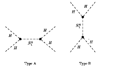
Figure 1: Diagrams type A and B which contribute to the effective couplings. External legs are bosons $H_{1,2}$ and the exchanged boson is the heavy $\tilde{N}_{1}^{0}$ field.

With the above definitions we see that the parts of the potential which contain $H_{1}$, $H_{2}$ and $\tilde{N}_{1}$ are

$$V^{\prime} = \frac{g^{2}}{6}\left[(\tilde{N}_{1}^{2})^{2}+(H_{1}^{\dagger}H_{1})^{2}+(H_{2}^{\dagger}H_{2})^{2}+3(\epsilon_{ij}H_{1}^{i}H_{2}^{j})^{2}\right.$$

$$- \left.\tilde{N}_{1}^{2}(H_{2}^{\dagger}H_{2})-(H_{1}^{\dagger}H_{1})(H_{2}^{\dagger}H_{2})+\tilde{N}_{1}^{2}(H_{1}^{\dagger}H_{1})\right]$$

$$+ \frac{g_{1}^{2}}{18}\left[4(H_{2}^{\dagger}H_{2})^{2}+(\tilde{N}_{1}^{2})^{2}+(H_{1}^{\dagger}H_{1})^{2}+2\tilde{N}_{1}^{2}(H_{1}^{\dagger}H_{1})\right.$$

$$- \left.4\tilde{N}_{1}^{2}(H_{2}^{\dagger}H_{2})-4(H_{1}^{\dagger}H_{1})(H_{2}^{\dagger}H_{2})\right]$$

$$+ h_{e}^{2}\left[(H_{1}^{\dagger}H_{1})(H_{2}^{\dagger}H_{2})-(\epsilon_{ij}H_{1}^{i}H_{2}^{j})^{2}+\tilde{N}_{1}^{2}(H_{2}^{\dagger}H_{2})+\tilde{N}_{1}^{2}(H_{1}^{\dagger}H_{1})\right].$$

The minimum conditions for the potential with the VEV $<\tilde{N}_{1}^{0}>=u$ and $<\tilde{N}_{3}^{0}>=u^{\prime}$ when $u^{\prime}$ goes to zero are satisfied if

$$m_{L\phi}^{2} = 0$$

$$m_{L}^{2} = -\left(\frac{{{g_{1}}}^{2}}{9}+\frac{{{g}}^{2}}{3}\right)\,u^{2}$$ (15)

and, therefore the mass of the field $\tilde{N}_{1}^{0}$ is given by $m_{N}^{2}=4\left(\frac{{{g_{1}}}^{2}}{9}+\frac{{{g}}^{2}}{3}\right)\,u^{2}$.

In the MSSM two scalar doublets appear, it is because their fermionic partners are necessary to cancel the axial-vector triangle anomalies. The requirement of SUSY also constrains the parameters of the Higgs potential. Therefore the Higgs potential of the MSSM can be seen as a special case of the more general 2HDM potential structure. This result in constraints among the $\lambda_{i}$’s of the general 2HDM potential [6, 11].

As it has been already emphasized [6], in the MSSM the quartic scalar couplings of the Higgs potential are completely determined in terms of the two gauge couplings, but it is not the case if the symmetry $SU(2)_{L}\otimes U(1)_{Y}$ is a remnant of a larger symmetry which is broken at a higher mass scale together with the SUSY. The structure of the Higgs potential is then determined by the scalar particle content needed to produce the spontaneous symmetry breaking. In this way, the reduced Higgs potential would be a 2HDM-like potential, but its quartic couplings would not be those of the MSSM. Instead, they will be related to the gauge couplings of the larger theory and to the couplings appearing in its superpotential. Analysis of supersymmetric theories in this context have been given in the literature [6, 12]. In particular, it has been studied widely for different versions of the left-right model and a specific SUSY version of the $SU(3)_{L}\otimes U(1)_{X}$ where exotic charged particles of electric charges $(-4/3,5/3)$ appear.

Following this idea with the reduced Higgs potential presented in the previous paragraphs, we can obtain the effective quartic scalar couplings $\lambda_{i}$ of the most general 2HDM potential. Since there are cubic interactions in $V^{\prime}$ involving $H_{1,2}$ and $\tilde{N}_{1}^{0}$, it generates two types of Feynman diagrams which contribute to the quartic couplings (figure 1). The Feynman rules from the potential for these couplings are

\begin{picture}(332.0,332.0)\put(0.0,0.0){}\put(332.0,332.0){}\ignorespaces\par\put(0.0,0.0){\raise 136.32645pt\hbox to0.0pt{\kern 66.64839pt\makebox(0.0,0.0)[b]{\small}\hss}}\ignorespaces\ignorespaces\ignorespaces\put(0.0,0.0){\raise 235.35138pt\hbox to0.0pt{\kern 33.93011pt\makebox(0.0,0.0)[tr]{$H_{2}$}\hss}}\ignorespaces\ignorespaces\put(0.0,0.0){\raise 180.82088pt\hbox to0.0pt{\kern 34.24113pt\makebox(0.0,0.0)[tl]{$H_{2}$}\hss}}\ignorespaces\ignorespaces\put(0.0,0.0){\raise 194.61345pt\hbox to0.0pt{\kern 196.9157pt\makebox(0.0,0.0)[b]{$i\left(\frac{-4\,{{g_{1}}}^{2}}{9}-\frac{{{g}}^{2}}{3}+2\,h_{e}^{2}\right)u$}\hss}}\ignorespaces\put(0.0,0.0){\raise 204.91373pt\hbox to0.0pt{\kern 93.91364pt\makebox(0.0,0.0)[b]{$\tilde{N}_{1}^{0}$}\hss}}\ignorespaces\ignorespaces\put(0.0,0.0){\raise 136.32645pt\hbox to0.0pt{\kern 199.94536pt\makebox(0.0,0.0)[b]{\small}\hss}}\ignorespaces\ignorespaces\put(0.0,0.0){\raise 3.02948pt\hbox to0.0pt{\kern 66.64839pt\makebox(0.0,0.0)[b]{\small}\hss}}\ignorespaces\ignorespaces\ignorespaces\put(0.0,0.0){\raise 102.05441pt\hbox to0.0pt{\kern 33.93011pt\makebox(0.0,0.0)[tr]{$H_{1}$}\hss}}\ignorespaces\ignorespaces\put(0.0,0.0){\raise 47.52391pt\hbox to0.0pt{\kern 34.24113pt\makebox(0.0,0.0)[tl]{$H_{1}$}\hss}}\ignorespaces\ignorespaces\put(0.0,0.0){\raise 61.31648pt\hbox to0.0pt{\kern 196.9157pt\makebox(0.0,0.0)[b]{$i\left(\frac{2{{g_{1}}}^{2}}{9}-\frac{{{g}}^{2}}{3}+2\,h_{e}^{2}\right)u$}\hss}}\ignorespaces\put(0.0,0.0){\raise 71.61676pt\hbox to0.0pt{\kern 93.91364pt\makebox(0.0,0.0)[b]{$\tilde{N}_{1}^{0}$}\hss}}\ignorespaces\ignorespaces\par\par\par\par\par\par\par\end{picture}

and using them we obtain the effective couplings, taking into account that the diagrams presented in figure 1 contribute to $\lambda_{1,2,3}$; thus they are given by

$$\frac{\lambda_{1}}{2} = \frac{g_{1}^{2}}{18}+\frac{g^{2}}{6}-\frac{3}{8}\left((\frac{2g_{1}^{2}}{9}-\frac{g^{2}}{3})^{2}+4h_{e}^{2}(\frac{2g_{1}^{2}}{9}-\frac{g^{2}}{3})+4h_{e}^{4}\right)G^{-1}\;\;,$$

$$\frac{\lambda_{2}}{2} = \frac{2g_{1}^{2}}{9}+\frac{g^{2}}{6}-\frac{3}{8}\left((\frac{4g_{1}^{2}}{9}+\frac{g^{2}}{3})^{2}-4h_{e}^{2}(\frac{4g_{1}^{2}}{9}+\frac{g^{2}}{3})+4h_{e}^{4}\right)G^{-1}\;\;,$$

$$\lambda_{3} = -\frac{2g_{1}^{2}}{9}-\frac{g^{2}}{6}+\frac{3}{4}\left((\frac{4g_{1}^{2}}{9}+\frac{g^{2}}{3})(\frac{2g_{1}^{2}}{9}-\frac{g^{2}}{3})\right.$$

$$+ \left.4h_{e}^{2}(\frac{g_{1}^{2}}{9}+\frac{g^{2}}{3})-4h_{e}^{4}\right)G^{-1}\;\;,$$

$$\lambda_{4} = \frac{g^{2}}{2}-h_{e}^{2}\;\;\;,\;\;\lambda_{5}=0$$ (16)

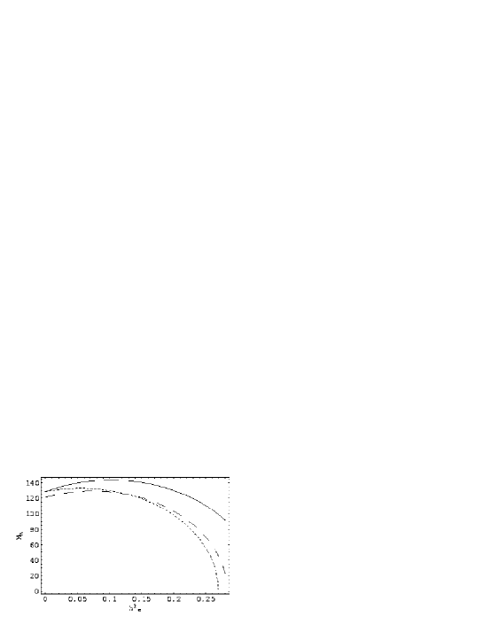
Figure 2: The upper bound on the lightest CP-even Higgs boson of the model as a function of the parameter $h_{e}^{2}$ from the superpotential. The solid, dashed and dotted lines correspond to $\cos^{2}\beta=\{0\;,\;0.6\;,\;1\}$ respectively.

where $G=\left(\frac{g_{1}^{2}}{3}+g^{2}\right)$. We want to remark that this SUSY model has the MSSM as an effective theory when the new physics is not longer there, $h_{e}=0$, and the coupling constants are running down to the electroweak scale. At this point we use the approach where the $SU(2)_{L}$ coupling behaves like $g$, and $g_{1}$ is the combination given by (6). In the limit $h_{e}^{2}=0$, we obtain

$$\lambda_{1,2}=\frac{g^{2}(4g_{1}^{2}+3g^{2})}{4(g_{1}^{2}+3g^{2})}\;\;,\;\;\lambda_{3}=-\frac{g^{2}(4g_{1}^{2}+3g^{2})}{4(g_{1}^{2}+3g^{2})}\,\,,\,\,\lambda_{4}=\frac{g^{2}}{2}$$

and, if we assume the matching condition from equation (6), we reduce the effective couplings to those appearing in the MSSM, as expected,

$$\lambda_{1}=\lambda_{2}=\frac{1}{4}(g^{2}+g^{\prime 2})\;\;,\;\;\lambda_{3}=-\frac{1}{4}(g^{2}+g^{\prime 2})\,\,,\,\,\lambda_{4}=\frac{g^{2}}{2}.$$

When we have the reduced Higgs potential, we should ask for the stability conditions. These conditions are well known [11] and they give us a constrain for the coupling $h_{e}$ which is a coupling in the superpotential of the larger symmetry and a new free parameter. The general requirement for $V$ to be bounded from below leads to the allowed region, $0\leq h_{e}^{2}\leq 0.28$.

On the other hand, for $\lambda_{5}=0$ in the potential, there is a general formula to obtain the upper bound on $M_{h}$ in the framework of a general Two Higgs Doublet Model [11, 6]. This formula is given in terms of the $\lambda_{i}$ parameters and we use it along with equation (18) in order to make plots in the $M_{h}$-$h_{e}^{2}$ plane. Figure 2 shows the plane $M_{h}$ versus $h_{e}^{2}$, for different values of $\cos^{2}\beta$, where $\beta$ is the CP-odd mixing angle. It is obvious that we can move the lower bound predicted by MSSM of about 128 GeV according to the values of the parameters involved in this model. In particular we get the upper bound of MSSM in the limit $h_{e}=0$. Further, we note from figure 2 that we can shift the upper bound up to a value of around 140 GeV for $h_{e}^{2}=0.1$ and $\cos\beta=0$. The upper bound on $M_{h}$ is consistent with the experimental bound from LEPII.

4 CONCLUSIONS

We have presented a new supersymmetric version of the gauge symmetry $SU(3)_{L}\otimes U(1)_{X}$ where the Higgs bosons correspond to the sleptons, and it is triangle anomaly free. The model has a number of free parameters which is smaller than other ones in the literature. We have also shown that using the limit when the parameter $h_{e}=0$ and the matching condition (equation (6)), we obtain the SUSY constraints for the Higgs potential as in the MSSM. Therefore, if we analyze the upper bound for the mass of the lightest CP-even Higgs boson in this limit, we find the same bound of around 128 GeV for the MSSM. However, since in general $h_{e}\not=0$, such upper bound can be moved up to around 140 GeV, see figure 2. This fact can be an interesting alternative to take into account in the search for the Higgs boson mass.

We acknowledge to D. Restrepo, W. Ponce and L. Sanchez for useful disscussions.This work was supported by COLCIENCIAS, DIB and Banco de la Republica.

References

- [1] S. Weinberg, Phys. Rev. Lett. 19 (1967) 1264; S. L. Glashow, Nucl. Phys. 20 (1961) 579; A. Salam, in: N. Svartholm (ed.), Elementary Particle Theory, 1968, p. 367.
- [2] C. H. Albright, C. Jarlskog and M. Tjia, Nucl. Phys. B86 (1974) 535 and references there in. F. Pisano and V. Pleitez, Phys. Rev. D. 46 (1992)410.
- [3] J.C. Montero, V. Pleitez, M.C. Rodriguez, Phys. Rev. D65 (2002) 095008, Phys. Rev. D. 65 (2002) 035006; M. Capdequi-Peyranere, M.C. Rodriguez, Phys. Rev. D. 65(2002) 035001.
- [4] M. Singer, J. F. W. Valle and Schechter, Phys. Rev. D. 22 (1980)738; R. Foot, H. N. Long and T.A. Tran, Phys. Rev. D. 50, R34 (1994); V. Pleitez, Phys. Rev. D. 53 (1996) 514.
- [5] R. Martinez, W. Ponce and L. A. Sanchez, Phys. Rev. D 65 (2002) 055013; Phys. Rev D 64 (2001) 075013; W. Ponce, J. Florez and L. A. Sanchez, Int. J. Mod. Phys. A 17 (2002) 643.
- [6] T. V. Duong and E. Ma, Phys. Lett. B 316 (1993) 307; E. Ma and D. Ng, Phys. Rev. D. 49 (1994) 6164.
- [7] H. Geogi, and D. V. Nanopoulos Phys. Lett. B82 (1979) 1.
- [8] LEPEWWG, hep-ex/0112021, http://lepewwg.web.cern.ch/LEPEWWG/
- [9] H. Haber and R. Hemplfling, Phys. Rev. Lett. 66 (1991) 1815; J. Ellis, G. Ridolfi and F. Zwirner, Phys. Lett. B 257 (1991) 83. R. Barbieri, M. Frigeni and F. Caravaglios, Phys. Lett. B 258 (1991) 167.
- [10] J. G. Branson, et. al., hep-ph/011021; D. Zeppenfeld, et.al., Phys. Rev. D 62 (2000) 0130009; A. Djouadi, W. Kilian, M. Muhlleitner and P.M. Zerwas, Eur. Phys. J. C 10 (1999) 45.
- [11] J. F. Gunion, H. Haber, G. Kane, S. Dawson, The Higgs hunter’s guide, Addison-Wesley, Redwood city, 1990.
- [12] K. S. Babu, X. G. He and E. Ma, Phys. Rev. D 36 (1987) 878; E. Ma, Phys. Rev. D 36 (1987) 274.