TU-666

CALT-68-2399

hep-ph/0208149

August, 2002

Top-Squark Study at a Future $e^{+}e^{-}$ Linear Collider

Ryuichiro Kitano^(a), Takeo Moroi^(a) and Shufang Su^(b)

^(a)Department of Physics, Tohoku University, Sendai 980-8578, Japan

^(b)California Institute of Technology, Pasadena, CA 91125, USA

We discuss a potential of studying the production and the decay of the lightest top squark ($\tilde{t}_{1}$) in the framework of the supersymmetric standard model at a future $e^{+}e^{-}$ collider. In particular, we consider the process $\tilde{t}_{1}\rightarrow t\chi^{0}_{1}$ (with $\chi^{0}_{1}$ being the lightest neutralino) followed by $t\rightarrow bW$. It is shown that, by the study of the angular distribution of the bottom quark (as well as the production cross section of the top squark), properties of $\chi_{1}^{0}$ can be extracted. We also discuss that, if $\chi^{0}_{1}$ is gaugino-like, the neutralino mixing parameters (i.e., the so-called $\mu$-parameter and $\tan\beta$) may be constrained.

1 Introduction

After the precise confirmation of the standard model of the elementary particles by the LEP, SLD, and Tevatron, main purpose of the high energy colliders are now shifting to discoveries and studies of new physics beyond the standard model. In particular, the Tevatron Run II and LHC experiments are expected to give us strong hints for studying the physics behind the electroweak symmetry breaking [1, 2]. As well as these hadron colliders, however, $e^{+}e^{-}$ linear colliders are an alternative possibility to study the physics at the electroweak scale. Indeed, $e^{+}e^{-}$ linear colliders are considered as serious candidates of the new program of experiments which pursue the energy frontier of the high energy physics [3, 4, 5, 6, 7].

Compared to the hadron colliders, $e^{+}e^{-}$ linear colliders may provide cleaner environments to study productions and decays of various particles with less background, which enables us to perform precision measurements of the particle properties. In addition, polarized $e^{-}$ beam will be available at $e^{+}e^{-}$ linear colliders which will be useful to study the properties of the new particles. Thus, $e^{+}e^{-}$ linear collider will play a complementary role in studying the physics beyond the standard model even if some signals of the new physics are discovered at the Tevatron Run II and/or the LHC before the start of $e^{+}e^{-}$ linear collider experiments. Therefore, it is important to understand what kind of information will be available from $e^{+}e^{-}$ linear colliders.

Among various possibilities, supersymmetry (SUSY) is one of the most attractive candidates of the new physics and hence it is significant to understand what can be studied at $e^{+}e^{-}$ linear colliders about SUSY models. The study is, however, not straightforward since there are many parameters in the model and the collider phenomenology crucially depends on these parameters. In the simplest set up, capabilities of $e^{+}e^{-}$ linear colliders have been well studied [8]. Most of the studies have, however, assumed some simple mass spectra of the superparticles. For a more complete understanding of the potential of $e^{+}e^{-}$ linear colliders, it is important to study various cases.

One of the possibilities is the case with a light stop (top squark). For the stops, due to the large top Yukawa coupling constant, effects of the left-right mixing in the mass matrix are expected to be large and one of the stops can become light. Thus, a light stop is easily realized in wide parameter space and hence it is important to consider what can be done with future high energy colliders. Since the stops affect the potential of the Higgs bosons through radiative corrections [9], stop study will provide useful information to understand the physics of the electroweak symmetry breaking. There has been several works on the stop productions and decays at future colliders. At $e^{+}e^{-}$ linear colliders, the determination of the mass and mixing of the stop from the stop-production cross section has been discussed in detail in Ref. [10] for a 180 GeV light stop by using the $\tilde{t}_{1}\to\chi_{1}^{0}c$ and $\tilde{t}_{1}\to\chi^{+}b$ modes. For the case of the LHC, it has been discussed that the end-point analysis of gluino decay processes is useful to understand properties of the stop [2, 11].

In this paper, we consider the case where the lightest stop $\tilde{t}_{1}$ is kinematically accessible at $e^{+}e^{-}$ linear colliders, while it is still heavy enough to be able to decay into top quark and the lightest neutralino $\chi^{0}_{1}$. In particular, we consider the pair production of the lightest stops and the decay of $\tilde{t}_{1}$ via $\tilde{t}_{1}\rightarrow t\chi^{0}_{1}$ followed by $t\rightarrow bW$, and discuss what can be studied. It will be shown that the stop mass and left-right mixing can be measured from the study of the production cross section with polarized beam. Also, the neutralino properties can be extracted by the analysis of the stop decay. The mass of the lightest SUSY particle (LSP) is determined from the end-point of the decay product of $\tilde{t}_{1}$. In addition, information on the neutralino mixing is obtained from the angular distribution of the $b$-jet. Similar analysis using the measurements of the polarization of $\tau$ from stau decays is proposed in Ref. [12]. The angular distribution of the $b$-jet carries information on the top-quark helicity. This fact enables us to extract neutralino mixing since the helicity of the top quark from the stop decay is related to the left-right stop mixing and the neutralino mixing effects, i.e., the gauginos (superpartner of gauge boson) couple left- and right-handed stops to left- and right-handed top quark, respectively, while the stop and top quark have opposite helicities at the Higgsino (superpartner of Higgs boson) vertices. It is also discussed that, for gaugino-like LSP, because of the large top Yukawa coupling constant, the angular distribution of the $b$-jet may depend on so-called $\mu$-parameter and hence our analysis provides some knowledge on $\mu$.

This paper is organized as follows. In Sec. 2, we briefly introduce the stop sector and the neutralino sector, presenting the mass and the mixing matrices. In Sec. 3, we illustrate how to determine the lightest-stop mass and mixing angle through the stop pair production with polarized electron beam. In Sec. 4, we discuss in detail the decay mode $\tilde{t}_{1}\rightarrow t\tilde{\chi}_{1}^{0}$, followed by $t\rightarrow bW$. The LSP mass can be obtained via the end-point of the energy distribution of the top quark. Sec. 5 is focusing on the angular distribution of the $b$-jet from the top decay, based on which we could obtain information on the neutralino mixing. We study three different neutralino LSP cases in Sec. 6, and show whether constrains on $\mu$ and $\tan\beta$ can be extracted. Sec. 7 is devoted to conclusions.

2 Top squark and neutralino sectors

In the minimal supersymmetric standard model (MSSM), there are two stops: $\tilde{t}_{L}$ and $\tilde{t}_{R}$, which are the superpartners of the left- and right-handed top quarks, respectively. After the electroweak symmetry breaking, these stops mix and become mass eigenstates. Mass matrix of the stops in the basis of $(\tilde{t}_{L},\tilde{t}_{R})$ is given by

$${\cal M}^{2}_{\tilde{t}}=\left(\begin{array}[]{cc}m_{\tilde{t}L}^{2}+m_{t}^{2}+D_{L}&-y_{t}\mu\langle H_{1}\rangle-A_{t}\langle H_{2}\rangle\\ -y_{t}\mu\langle H_{1}\rangle-A_{t}\langle H_{2}\rangle&m_{\tilde{t}R}^{2}+m_{t}^{2}+D_{R}\end{array}\right),$$ (3)

where $m_{\tilde{t}L}^{2}$ and $m_{\tilde{t}R}^{2}$ are the soft SUSY breaking mass parameters for the left- and right-handed stops, respectively, $y_{t}$ is the top Yukawa coupling constant, $m_{t}$ the top quark mass, $\mu$ the SUSY invariant Higgs mass, and $A_{t}$ the tri-linear coupling constant of stop. For simplicity, we assume that all the SUSY parameters are real in our analysis. In addition, $H_{1}$ and $H_{2}$ are down- and up-type Higgs bosons, respectively, and $\langle\cdots\rangle$ is the vacuum expectation value. The $D$-term contributions $D_{L}$ and $D_{R}$ are given by

$$D_{L}=\left(\frac{g_{2}^{2}}{4}-\frac{g_{1}^{2}}{12}\right)\left(\langle H_{1}\rangle^{2}-\langle H_{2}\rangle^{2}\right),~{}~{}~{}D_{R}=\frac{g_{1}^{2}}{3}\left(\langle H_{1}\rangle^{2}-\langle H_{2}\rangle^{2}\right),$$ (4)

where $g_{1}$ and $g_{2}$ are the gauge coupling constants of the U(1)_Y and SU(2)_L gauge interactions, respectively.

The stop mass matrix ${\cal M}^{2}_{\tilde{t}}$ can be diagonalized by the unitary matrix $U_{\tilde{t}}$ to give mass eigenstates $\tilde{t}_{1}$ and $\tilde{t}_{2}$:

$$\left(\begin{array}[]{c}\tilde{t}_{1}\\ \tilde{t}_{2}\end{array}\right)=U_{\tilde{t}}\left(\begin{array}[]{c}\tilde{t}_{L}\\ \tilde{t}_{R}\end{array}\right)=\left(\begin{array}[]{cc}\cos\theta_{\tilde{t}}&\sin\theta_{\tilde{t}}\\ -\sin\theta_{\tilde{t}}&\cos\theta_{\tilde{t}}\end{array}\right)\left(\begin{array}[]{c}\tilde{t}_{L}\\ \tilde{t}_{R}\end{array}\right),$$ (13)

with mass eigenvalues $m_{\tilde{t}_{1}}^{2}$ and $m_{\tilde{t}_{2}}^{2}$. $\theta_{\tilde{t}}$ is the mixing angle that parametrizes the left-right stop mixing. (We define $m_{\tilde{t}_{1}}<m_{\tilde{t}_{2}}$ and $-\frac{\pi}{2}\leq\theta_{\tilde{t}}\leq\frac{\pi}{2}$.) With this definition, the lightest stop becomes purely left-handed if $\theta_{\tilde{t}}=0$ and right-handed if $\theta_{\tilde{t}}=\frac{\pi}{2}$ and $-\frac{\pi}{2}$. The left-right mixing in the stop sector could be sizable due to the large top Yukawa coupling constant. Consequently, the mass of the lightest stop $\tilde{t}_{1}$ could be so small that pair production of $\tilde{t}_{1}\tilde{t}_{1}^{*}$ is kinematically allowed at $e^{+}e^{-}$ linear colliders.

For the neutralino sector, Bino $\tilde{B}$, neutral Wino $\tilde{W}$, neutral down-type Higgsino $\tilde{H}_{1}$, and neutral up-type Higgsino $\tilde{H}_{2}$ are mixed together to form mass eigenstates. Mass matrix of the neutralinos in the basis of $(\tilde{B},\tilde{W},\tilde{H}_{1},\tilde{H}_{2})$ is given by

$${\cal M}_{\chi^{0}}=\left(\begin{array}[]{cccc}M_{1}&0&\frac{1}{\sqrt{2}}g_{1}\langle H_{1}\rangle&-\frac{1}{\sqrt{2}}g_{1}\langle H_{2}\rangle\\ 0&M_{2}&-\frac{1}{\sqrt{2}}g_{2}\langle H_{1}\rangle&\frac{1}{\sqrt{2}}g_{2}\langle H_{2}\rangle\\ \frac{1}{\sqrt{2}}g_{1}\langle H_{1}\rangle&-\frac{1}{\sqrt{2}}g_{2}\langle H_{1}\rangle&0&-\mu\\ -\frac{1}{\sqrt{2}}g_{1}\langle H_{2}\rangle&\frac{1}{\sqrt{2}}g_{2}\langle H_{2}\rangle&-\mu&0\end{array}\right),$$ (18)

where $M_{1}$ and $M_{2}$ are the U(1)_Y and SU(2)_L gaugino masses, respectively. The mass matrix ${\cal M}_{\chi^{0}}$ can be diagonalized by a unitary matrix $U_{\chi^{0}}$, such that

$${\cal M}_{\chi^{0}}^{\rm diag}=U_{\chi^{0}}{\cal M}_{\chi^{0}}U_{\chi^{0}}^{T}.$$ (19)

The mass eigenstate of neutralino $\chi^{0}_{i}$ is thus given by

$$\chi^{0}_{i}=[U_{\chi^{0}}]^{*}_{i\tilde{B}}\tilde{B}+[U_{\chi^{0}}]^{*}_{i\tilde{W}}\tilde{W}+[U_{\chi^{0}}]^{*}_{i\tilde{H}_{1}}\tilde{H}_{1}+[U_{\chi^{0}}]^{*}_{i\tilde{H}_{2}}\tilde{H}_{2},$$ (20)

with $\chi_{1}^{0}$ being the lightest neutralino (i.e., the LSP in our analysis). The neutralino mass eigenvalues $m_{\chi_{i}^{0}}$ and mixing matrix $U_{\chi^{0}}$ are determined by four parameters $M_{1}$, $M_{2}$, $\mu$ and $\tan\beta$. Considering the case where $\langle H_{1}\rangle,\langle H_{1}\rangle\ll|M_{1}|,|M_{2}|,|\mu|$, the neutralino mass eigenstates are nearly $\tilde{B}$, $\tilde{W}$, $(\tilde{H}_{1}\pm\tilde{H}_{2})/\sqrt{2}$, with mass eigenvalues $\sim$ $|M_{1}|$, $|M_{2}|$ and $|\mu|$. Depending on the relative magnitude of $|M_{1}|$, $|M_{2}|$ and $|\mu|$, we would have Bino-like, Wino-like or Higgsino-like lightest neutralino as the LSP.

As one can see, the mass matrices of the stops and the neutralinos depend on various SUSY parameters. Thus the mass spectrum of the superparticles is really model dependent. In this paper, to make our points clear, we assume that the lightest stop $\tilde{t}_{1}$ is accessible at $e^{+}e^{-}$ linear colliders but the heavier one $\tilde{t}_{2}$ is not.

3 Stop pair production

Let us first consider the pair production process of the lightest stop. Importantly, it is expected that the electron beam can be polarized at future $e^{+}e^{-}$ linear colliders, which is extremely useful for the study of the stops [10]. The production cross section with the left-polarized electron beam is given by

$$\sigma(e^{+}e_{L}^{-}\rightarrow\tilde{t}_{1}\tilde{t}^{*}_{1})=\frac{1}{16\pi s}\left(Q_{e}Q_{t}+g^{e_{L}}_{Z}g^{\tilde{t}_{1}}_{Z}\frac{s}{s-m_{Z}^{2}}\right)^{2}\left(1-\frac{4m_{\tilde{t}_{1}}^{2}}{s}\right)^{3/2},$$ (21)

where $\sqrt{s}$ is the center of mass energy of the linear collider. Similar formula for $\sigma(e^{+}e_{R}^{-}\rightarrow\tilde{t}_{1}\tilde{t}^{*}_{1})$ is obtained by replacing $L\rightarrow R$. The charges and couplings in Eq. (21) are given by

$$Q_{e}=-e,~{}~{}~{}g^{e_{L}}_{Z}=\frac{-g_{2}^{2}+g_{1}^{2}}{2g_{Z}},~{}~{}~{}g^{e_{R}}_{Z}=\frac{g_{1}^{2}}{g_{Z}},$$ (22)

and

$$Q_{t}=\frac{2}{3}e,~{}~{}~{}g^{\tilde{t}_{1}}_{Z}=\frac{1}{g_{Z}}\left(\frac{1}{2}g_{2}^{2}-\frac{1}{6}g_{1}^{2}\right)\cos^{2}\theta_{\tilde{t}}-\frac{2g_{1}^{2}}{3g_{Z}}\sin^{2}\theta_{\tilde{t}},$$ (23)

where $g_{Z}=\sqrt{g_{2}^{2}+g_{1}^{2}}$, $e=g_{1}g_{2}/g_{Z}$, and $m_{Z}$ is the $Z$-boson mass.

Diagrams with photon-exchange and $Z$-exchange both contribute to the production cross section, which interfere either constructively or destructively depending on the polarization of the electron beam and the stop mixing angle.

Figure 1: Contours of constant $\sigma(e^{+}e^{-}_{L}\rightarrow\tilde{t}_{1}\tilde{t}^{*}_{1})$ (left plot) and $\sigma(e^{+}e^{-}_{R}\rightarrow\tilde{t}_{1}\tilde{t}^{*}_{1})$ (right plot) on the $m_{\tilde{t}_{1}}$ vs. $|\tan\theta_{\tilde{t}}|$ plane at a linear collider with center-of-mass energy $\sqrt{s}=1\ {\rm TeV}$.

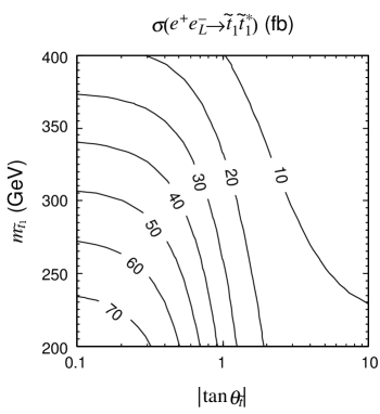
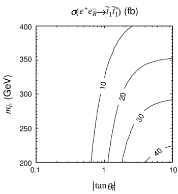
In Fig. 1, we plot the contours of constant $\sigma(e^{+}e^{-}_{L}\rightarrow\tilde{t}_{1}\tilde{t}^{*}_{1})$ and $\sigma(e^{+}e^{-}_{R}\rightarrow\tilde{t}_{1}\tilde{t}^{*}_{1})$ on the $m_{\tilde{t}_{1}}$ vs. $|\tan\theta_{\tilde{t}}|$ plane. (Here and hereafter, we take $\sqrt{s}=1\ {\rm TeV}$.) The cross sections are sensitive to both the mass and mixing of the stop, as expected. The behaviors of the cross sections can be understood in the following way. With left-polarized electron beam, photon and $Z$-exchange diagrams interfere constructively when the lightest stop is almost left-handed (i.e., when $|\tan\theta_{\tilde{t}}|$ is small), and destructively when the lightest stop is almost right-handed. Such effect is shown in the left plot of Fig. 1; the cross section decreases as $|\tan\theta_{\tilde{t}}|$ increases. With right-polarized beam, the interference term flips sign. Therefore, the cross section increases as $|\tan\theta_{\tilde{t}}|$ increases, which is shown in the right plot of Fig. 1.

Most importantly, both $m_{\tilde{t}_{1}}$ and $\theta_{\tilde{t}}$ can be determined simultaneously using the cross-section measurement with polarized beam [10, 13, 14] since dependences of $\sigma(e^{+}e^{-}_{L}\rightarrow\tilde{t}_{1}\tilde{t}^{*}_{1})$ and $\sigma(e^{+}e^{-}_{R}\rightarrow\tilde{t}_{1}\tilde{t}^{*}_{1})$ on $m_{\tilde{t}_{1}}$ and $\theta_{\tilde{t}}$ are significantly different. (See Fig. 1.)

In the following analysis, we use the averaged cross section in estimating the number of events:

$$\sigma=\frac{1}{2}\left[\sigma(e^{+}e^{-}_{L}\rightarrow\tilde{t}_{1}\tilde{t}^{*}_{1})+\sigma(e^{+}e^{-}_{R}\rightarrow\tilde{t}_{1}\tilde{t}^{*}_{1})\right].$$ (24)

4 Stop decay

Given that we have known the value of $m_{\tilde{t}_{1}}$ and $\theta_{\tilde{t}}$ from the measurements of the stop production cross sections, we now study whether the stop decay renders additional information on the stop and neutralino sectors. In our analysis, we use the decay mode $\tilde{t}_{1}\rightarrow t\chi^{0}_{1}$ followed by $t\rightarrow bW$. Reconstruction of the top quark events provides us energy distribution of the top quark and angular distribution of the $b$-jet. The former may be used to obtain the mass of the LSP. In addition, the latter is sensitive to helicity of the top quark which depends on the LSP properties. Therefore, the angular distribution of the $b$-jet can be used to extract informations on the LSP.

Classifying the decay modes of the $W$-boson, the possible final states of the $\tilde{t}_{1}\tilde{t}^{*}_{1}$ production process are:

• $2b$ + $4q$ + missing momentum (48 %),

• $2b$ + $2q$ + $1l$ + missing momentum (43 %),

• $2b$ + $2l$ + missing momentum (9 %),

where $b$ and $q$ are hadronic jets with and without a $b$-tag, respectively, and $l$ is the charged lepton. With the vertex detector, we expect that the $b$-jet will be distinguished from other hadronic activities with high efficiency. In order to carry out the analysis of the stop decay, at least one of the $W$-boson should decay hadronically so that the top quark can be reconstructed. Thus, the events with final states (a) and (b) are used for the following analysis.

We assume that there is no SUSY background, and we expect the standard-model backgrounds from the following processes [15]:

• $t\bar{t}Z$ followed by $Z\rightarrow\nu\bar{\nu}$ ($\sim 1\ {\rm fb}$)

• $t\bar{t}\nu_{e}\bar{\nu}_{e}$ ($\sim 0.5\ {\rm fb}$)

• $ZW^{\pm}W^{\mp}$ followed by $Z\rightarrow b\bar{b}$, $W^{\pm}\rightarrow l\bar{\nu}$, and $W^{\mp}\rightarrow{\rm hadrons}$ ($\sim 3\ {\rm fb}$)

• $e^{\pm}\nu_{e}(\bar{\nu}_{e})W^{\mp}Z$ followed by $Z\rightarrow b\bar{b}$, and $W\rightarrow{\rm hadrons}$ ($\sim 11\ {\rm fb}$)

We assume that the backgrounds (iii) and (iv) can be eliminated by imposing relevant cut since the invariant mass of two $b$-jets is equal to $m_{Z}$. On the contrary, the processes (i) and (ii) provide irreducible backgrounds. These are, however, standard-model processes and hence their cross sections are calculable. Therefore, we can subtract the number of backgrounds from the number of signal candidates in the measurements of the cross sections. In addition, the cross sections for these processes are order-of-magnitude smaller than the signal cross section. Thus, as we will see later, effects of these backgrounds are insignificant.

In a stop pair production event, if all the lightest stop decays into $t$ and $\chi_{1}^{0}$, the averaged number of stops available for the analysis (process (a) and (b)) is

$$\epsilon=2\epsilon_{b}^{2}Br(W\rightarrow{\rm had.}),$$ (25)

where $\epsilon_{b}$ is the efficiency of the $b$-tagging and $Br(W\rightarrow{\rm had.})\simeq 0.69$ is the hadronic branching ratio of the $W$-boson. With $\epsilon_{b}=60\ \%$ [6], we use $\epsilon\simeq 0.50$. Notice that if additional stop decay modes are available, for example, $\tilde{t}_{1}\rightarrow b\chi_{1}^{\pm}$ in Wino-LSP and Higgsino-LSP case, $\epsilon$ should be multiplied by an additional factor of $Br(\tilde{t}_{1}\rightarrow t\chi_{1}^{0})$. In this case, measurement of the branching ratio of $\tilde{t}_{1}$ provides additional information on the neutralino/chargino sector.

Once the top quark from the decay of $\tilde{t}_{1}$ is reconstructed, the mass of the LSP can be determined by measuring the energy distribution of the top quark. Indeed, the maximum and minimum energy of the top quark in the lab frame, $E_{t}^{\rm(max)}$ and $E_{t}^{\rm(min)}$, respectively, are given by

$$E_{t}^{\rm(max)}=\frac{E_{t}^{*}+p_{t}^{*}\beta_{\tilde{t}_{1}}}{\sqrt{1-\beta_{\tilde{t}_{1}}^{2}}},~{}~{}~{}E_{t}^{\rm(min)}=\frac{E_{t}^{*}-p_{t}^{*}\beta_{\tilde{t}_{1}}}{\sqrt{1-\beta_{\tilde{t}_{1}}^{2}}},$$ (26)

where

$$E_{t}^{*}=\frac{m_{\tilde{t}_{1}}^{2}-m_{\chi^{0}_{1}}^{2}+m_{t}^{2}}{2m_{\tilde{t}_{1}}},~{}~{}~{}p_{t}^{*}=\sqrt{(E_{t}^{*})^{2}-m_{t}^{2}},$$ (27)

and $\beta_{\tilde{t}_{1}}=(1-4m_{\tilde{t}_{1}}^{2}/s)^{1/2}$. By measuring these end-points, we obtain information about the mass of the LSP (as well as that about the stop mass) [13]. At this stage, the parameters $m_{\tilde{t}_{1}}$, $\theta_{\tilde{t}}$, and $m_{\chi^{0}_{1}}$ are determined from the stop production cross sections and stop decay kinematics. In the following analysis, we assume that these three parameters are well understood.

5 Angular distribution of $b$-jet

Stop couples to the gauginos and to up-type Higgsino through the gauge and Yukawa interactions, respectively. One striking difference between the couplings to the gauginos and that to the Higgsino is that the left-handed (right-handed) stop couples only to left-handed (right-handed) top quark via gaugino interactions, while the helicity is flipped via the Higgsino interaction. Therefore, information about the stop and the LSP is imprinted in the helicity of the top quark and hence the measurement of the helicity of the top quark provides some knowledge of these particles. This point becomes clearer by looking at the top-stop-neutralino vertex. The coupling of the lightest stop $\tilde{t}_{1}$ with the top and the lightest neutralino is given by

$${\cal L}_{\rm int} = \tilde{t}_{1}^{*}\bar{\chi}^{0}_{1}(f_{L}P_{L}+f_{R}P_{R})t+\tilde{t}_{1}\bar{t}(f_{L}^{*}P_{R}+f_{R}^{*}P_{L})\chi^{0}_{1},$$ (28)

where $P_{L/R}=\frac{1}{2}(1\mp\gamma_{5})$, respectively, and

$$f_{L} = \left[\frac{1}{\sqrt{2}}g_{2}[U_{\chi^{0}}]_{1\tilde{W}}+\frac{1}{3\sqrt{2}}g_{1}[U_{\chi^{0}}]_{1\tilde{B}}\right]\cos\theta_{\tilde{t}}-y_{t}[U_{\chi^{0}}]_{1\tilde{H}_{2}}\sin\theta_{\tilde{t}},$$ (29)

$$f_{R} = -\frac{2\sqrt{2}}{3}g_{1}[U_{\chi^{0}}]^{*}_{1\tilde{B}}\sin\theta_{\tilde{t}}-y_{t}[U_{\chi^{0}}]^{*}_{1\tilde{H}_{2}}\cos\theta_{\tilde{t}}.$$ (30)

Thus, for the case where the lightest stop is $\tilde{t}_{L}$, for example, the top quark becomes left-handed if $\chi^{0}_{1}$ is gaugino-like while it becomes right-handed if $\chi^{0}_{1}$ is Higgsino-like.

In order to measure the helicity of the top quark, it is efficient to study the angular distribution of decay products from the top, like the $b$-quark [16]. The angular distribution of $b$-jet from the decay of a top quark with certain helicity can be obtained via direct computation, or by using the spin vector method. Here we use the latter. With Eq. (28), the spin vector $S^{\mu}$ for the top quark in the decay process $\tilde{t}_{1}\rightarrow t\chi^{0}_{1}$ is given by

$$\frac{1}{2}N(\not{\hbox{\kern-3.0pt$P$}}_{t}+m_{t})(1+\not{\hbox{\kern-3.0pt$S$}}\gamma_{5})$$

$$\equiv(\not{\hbox{\kern-3.0pt$P$}}_{t}+m_{t})(f_{L}^{*}P_{R}+f_{R}^{*}P_{L})(\not{\hbox{\kern-3.0pt$P$}}_{\chi}-m_{\chi^{0}_{1}})(f_{L}P_{L}+f_{R}P_{R})(\not{\hbox{\kern-3.0pt$P$}}_{t}+m_{t}),$$ (31)

with $P_{t}$ and $P_{\chi}$ being four-momenta of the top quark and the LSP, respectively. Then,

$$N = (m_{\tilde{t}_{1}}^{2}-m_{t}^{2}-m_{\chi^{0}_{1}}^{2})(|f_{L}|^{2}+|f_{R}|^{2})-4m_{t}m_{\chi^{0}_{1}}{\rm Re}(f_{L}^{*}f_{R}),$$ (32)

$$NS^{\mu} = -\frac{1}{m_{t}}\left[2m_{t}^{2}P_{\chi}^{\mu}-(m_{\tilde{t}_{1}}^{2}-m_{t}^{2}-m_{\chi^{0}_{1}}^{2})P_{t}^{\mu}\right](|f_{L}|^{2}-|f_{R}|^{2}).$$ (33)

For the process $\tilde{t}_{1}\rightarrow t\chi^{0}_{1}$ followed by $t\rightarrow bW$, the angular distribution of the $b$-jet in the rest frame of the top quark is given by

$$\frac{1}{\Gamma_{\tilde{t}}}\frac{d\Gamma_{\tilde{t}}}{d\cos\theta_{tb}}\equiv\frac{1}{2}(1+A_{b}\cos\theta_{tb}),$$ (34)

where $\theta_{tb}$ is the angle between top and bottom quark jets in the rest frame of the top quark, and the coefficient $A_{b}$ is related to the spin vector $S^{\mu}$ via

$$A_{b}=-\frac{m_{t}^{2}-2m_{W}^{2}}{m_{t}^{2}+2m_{W}^{2}}\hat{S}_{t},$$ (35)

with

$$\hat{S}_{t} = -\frac{2m_{t}|{\bf P_{\chi}}|}{N}(|f_{L}|^{2}-|f_{R}|^{2})$$ (36)

$$= -\frac{[m_{\tilde{t}_{1}}^{2}-(m_{t}-m_{\chi^{0}_{1}})^{2}]^{1/2}[m_{\tilde{t}_{1}}^{2}-(m_{t}+m_{\chi^{0}_{1}})^{2}]^{1/2}}{(m_{\tilde{t}_{1}}^{2}-m_{t}^{2}-m_{\chi^{0}_{1}}^{2})(|f_{L}|^{2}+|f_{R}|^{2})-4m_{t}m_{\chi^{0}_{1}}{\rm Re}(f_{L}^{*}f_{R})}(|f_{L}|^{2}-|f_{R}|^{2}).$$

Here ${\bf P}_{\chi}$ is the three-momentum of the LSP in the rest frame of the top quark and $\hat{S}_{t}^{2}=-S^{\mu}S^{\mu}$. Notice that $A_{b}$ depends only on $f_{L}/f_{R}$ and there is a two-fold degeneracy.

We can also obtain the angular distribution of the $s$-jets assuming that the $W$-boson decays into $c$ and $s$:

$$\frac{1}{\Gamma_{\tilde{t}}}\frac{d\Gamma_{\tilde{t}}}{d\cos\theta_{ts}}\equiv\frac{1}{2}(1+A_{s}\cos\theta_{ts}),$$ (37)

with

$$A_{s}=\hat{S}_{t}.$$ (38)

In this case, there is no suppression factor which appears in Eq.(35). However, it is difficult to directly identify the $s$-jet, although one possibility may be to tag the $c$-jet as well as $b$-jet. Thus, we believe it is challenging to measure $A_{s}$ and, in the following, we concentrate on the analysis of $A_{b}$.

Figure 2: $A_{b}$ as a function of $\tan\theta_{L/R}=f_{L}/f_{R}$. Here, we take $\sqrt{s}=1\ {\rm TeV}$, and the stop and neutralino masses are taken to be $m_{\tilde{t}_{1}}=300$ GeV and $m_{\chi^{0}_{1}}=100$ GeV (solid line), $m_{\tilde{t}_{1}}=350$ GeV and $m_{\chi^{0}_{1}}=100$ GeV (dash-dotted line), and $m_{\tilde{t}_{1}}=400$ GeV and $m_{\chi^{0}_{1}}=200$ GeV (dashed line).

Given the fact that it is difficult to measure the total decay width of $\tilde{t}_{1}$, the only information is given in the form of the angular distribution of the bottom quark from the decay chain of $\tilde{t}_{1}$. Even so, the ratio $f_{L}/f_{R}$ can be, in principle, determined and hence we obtain the information about the properties of the stop and the LSP. Indeed, the $A_{b}$-parameter has strong dependence on the ratio $f_{L}/f_{R}$. In Fig. 2, we plot $A_{b}$ as a function of $f_{L}/f_{R}$ for several values of $m_{\tilde{t}_{1}}$ and $m_{\chi^{0}_{1}}$. Here, we define the angle $\theta_{L/R}$ as

$$\tan\theta_{L/R}=f_{L}/f_{R}.$$ (39)

$A_{b}$ is asymmetric with respect to the sign of $\theta_{L/R}$ because of the ${\rm Re}(f_{L}^{*}f_{R})$ term in the denominator of Eq. (36). As one can see, $A_{b}$ changes from about $-0.4$ to $0.4$ as $\theta_{L/R}$ varies; the steepest dependence on $\theta_{L/R}$ occurs around $\theta_{L/R}\sim\pi/4$ (i.e., $f_{L}/f_{R}\sim 1$). Thus, measurement of the $A_{b}$-parameter provides constraint on the ratio $f_{L}/f_{R}$ although, unfortunately, the two-fold ambiguity always remains.

In order to discuss the statistical uncertainties in the measurement of $A_{b}$, we express $A_{b}$ in terms of numbers of signal events $N_{\rm S}^{\pm}$, where the superscripts “$+$” and “$-$” are for the events with $\cos\theta_{tb}>0$ and $\cos\theta_{tb}<0$, respectively: $N_{\rm S}^{\pm}\propto 1/2\pm A_{b}/4$. Similarly, we define number of the background events as $N_{\rm B}^{\pm}$. With these variables, total number of events are given by $N_{\rm tot}^{\pm}=N_{\rm S}^{\pm}+N_{\rm B}^{\pm}$, and the $A_{b}$-parameter is expressed as

$$A_{b}=\frac{2(N_{\rm S}^{+}-N_{\rm S}^{-})}{N_{\rm S}^{+}+N_{\rm S}^{-}}=\frac{2(N_{\rm tot}^{+}-N_{\rm tot}^{-})-2(N_{\rm B}^{+}-N_{\rm B}^{-})}{N_{\rm tot}-N_{\rm B}},$$ (40)

where $N_{\rm tot}=N_{\rm tot}^{+}+N_{\rm tot}^{-}$ and $N_{\rm B}=N_{\rm B}^{+}+N_{\rm B}^{-}$. Notice that $N_{\rm B}^{\pm}$ are calculable quantities. Then, the statistical uncertainty in the measurement of $A_{b}$ is estimated to be

$$(\delta A_{b})^{2}=\frac{16[N_{\rm tot}^{+}(N_{\rm tot}^{-}-N_{\rm B}^{-})^{2}+N_{\rm tot}^{-}(N_{\rm tot}^{+}-N_{\rm B}^{+})^{2}]}{(N_{\rm tot}-N_{\rm B})^{4}}\simeq\frac{4}{N_{\rm tot}},$$ (41)

where, in the second equality, we use the relations $N_{\rm B}\ll N_{\rm tot}$ and $A_{b}^{2}\ll 1$. Without these simplifications, $(\delta A_{b})^{2}$ increases about 10 %.

Constraints on the $A_{b}$-parameter can be translated to the bound on the ratio $f_{L}/f_{R}$. In order to estimate the expected bound on $f_{L}/f_{R}$ for a certain underlying value of $f_{L}/f_{R}$, we first fix the masses ($m_{\tilde{t}_{1}}$ and $m_{\chi^{0}_{1}}$) and the stop mixing angle $\theta_{\tilde{t}}$. Then, we determine $A_{b}$ with Eqs. (35) and (36) by inputting the underlying value of $f_{L}/f_{R}$. Simultaneously, with neglecting the backgrounds, we calculate the total number of events $N_{\rm tot}=\epsilon L\sigma$ for a given integrated luminosity $L$ and estimate the uncertainty of $A_{b}$ using Eq. (41). Then, to put the bound, we postulate the hypothetical value of $f_{L}/f_{R}$ and calculate $A_{b}$, and determine if such a value is within the experimental bound on $A_{b}$.

In Fig. 3, we plot the expected upper and lower bounds on $\theta_{L/R}$ as a function of the input value of $\theta_{L/R}$. Here, we take $m_{\tilde{t}_{1}}=350\ {\rm GeV}$, $\theta_{\tilde{t}}=\pi/4$, $m_{\chi^{0}_{1}}=100\ {\rm GeV}$, and $L=100\ {\rm fb}^{-1}$ (left plot) and $L=1000\ {\rm fb}^{-1}$ (right plot). With these parameters, the total number of events is given by $N_{\rm tot}\simeq 650$ ($L=100\ {\rm fb}^{-1}$) and 6500 ($L=1000\ {\rm fb}^{-1}$), which give $\delta A_{b}\simeq 0.08$ and 0.02, respectively.

For one $\theta_{L/R}^{\rm input}$, there are two possible regions of $\theta_{L/R}^{\rm output}$, due to the two-fold ambiguities that we mentioned earlier. For $\theta_{L/R}^{\rm input}$ close to 0 and $\pi/2$, which corresponds to the region where $A_{b}$ is at its minimum or maximum, two regions merge. In the case of $\theta_{L/R}>0$, higher precision is obtained compared to the case of $\theta_{L/R}<0$ since the $A_{b}$ dependence on $\theta_{L/R}$ becomes steeper when $\theta_{L/R}$ is positive. With $L=100\ {\rm fb}^{-1}$, the uncertainty of $\theta_{L/R}/\pi$ can be as small as 0.05 (0.1) at 1-$\sigma$ (2-$\sigma$) although the two-fold ambiguity exists.

Figure 3: Expected upper and lower bounds at 1-$\sigma$ (solid line) and 2-$\sigma$ (dashed line) level on $\theta_{L/R}$ as a function of the input-value of $\theta_{L/R}$. We take $m_{\tilde{t}_{1}}=350\ {\rm GeV}$, $\theta_{\tilde{t}}=\pi/4$, and $m_{\chi^{0}_{1}}=100\ {\rm GeV}$. The total numbers of events $N_{\rm tot}$ are set to be $650$ and $6500$ corresponding to $L=100$ fb^-1 (left plot) and $1000$ fb^-1 (right plot), respectively.

6 $\mu$-parameter

Since the parameters $m_{\tilde{t}_{1}}$, $\theta_{\tilde{t}}$, and $m_{\chi^{0}_{1}}$ are determined without information about $A_{b}$, the measurement of $\theta_{L/R}$, which depends on the neutralino mixing matrix $U_{\chi^{0}}$, can be used to study the neutralino sector. However, information we could obtain depends on what the lightest neutralino is. So, we consider the three typical cases: Bino-like LSP, Wino-like LSP, and Higgsino-like LSP cases. To make our point clear, we assume that the lightest stop can decay only into one of the Bino-like, Wino-like, or Higgsino-like particles (including chargino). Such a situation is realized when there is some hierarchy among the parameters $M_{1}$, $M_{2}$, and $\mu$.

Figure 4: $A_{b}$ as a function of $\mu$-parameter for $\tan\theta_{\tilde{t}}=-1$, $-0.5$, $0$, $0.5$, $1$. We take $\tan\beta=10$, $m_{\tilde{t}_{1}}=400$ GeV, $m_{\chi_{1}^{0}}=200$ GeV, and $M_{2}=500$ GeV.

6.1 Bino-like LSP

Even if the LSP is “Bino-like,” there can be sizable contaminations of the Higgsino components in the LSP which affect the $f_{L}$- and $f_{R}$-parameters. It is instructive to consider the case $\langle H_{1}\rangle,\langle H_{2}\rangle\ll|M_{1}|,|M_{2}|,|\mu|$ in order to study effects of the Higgsino components. In this case, the mixing matrix elements are approximately given by $[U_{\chi^{0}}]_{1\tilde{B}}\simeq 1$, $[U_{\chi^{0}}]_{1\tilde{W}}\simeq 0$,

$$[U_{\chi^{0}}]_{1\tilde{H}_{1}}\simeq-\frac{m_{Z}\sin\theta_{W}(M_{1}\cos\beta+\mu\sin\beta)}{\mu^{2}-M_{1}^{2}},$$ (42)

and

$$[U_{\chi^{0}}]_{1\tilde{H}_{2}}\simeq\frac{m_{Z}\sin\theta_{W}(M_{1}\sin\beta+\mu\cos\beta)}{\mu^{2}-M_{1}^{2}},$$ (43)

where $\sin\theta_{W}$ is the weak mixing angle and $\tan\beta$ is the ratio of the two vacuum expectation values of the Higgs fields, i.e., $\tan\beta=\langle H_{2}\rangle/\langle H_{1}\rangle$. Thus, even if $[U_{\chi^{0}}]_{1\tilde{B}}$ is close to 1, $[U_{\chi^{0}}]_{1\tilde{H}_{2}}\sim O(0.1)$ is possible in a large parameter space. In addition, it is important to note that $y_{t}$ is large and hence the Higgsino contributions to the coupling constants $f_{L}$ and $f_{R}$ are enhanced. Since $[U_{\chi^{0}}]_{1\tilde{H}_{2}}$ has strong dependence on $\mu$, the $\mu$-parameter may be constrained from the measurement of $A_{b}$. $[U_{\chi^{0}}]_{1\tilde{H}_{2}}$ also depends on $\tan\beta$ when $\tan\beta$ is small. On the contrary, when $\tan\beta$ is large, the $\tan\beta$ dependence becomes weak.

In Fig. 4, we plot $A_{b}$ as a function of $\mu$ for several values of $\tan\theta_{\tilde{t}}$. As expected, $A_{b}$ varies depending on the value of $\theta_{\tilde{t}}$. More interestingly, when $-0.5\lesssim\tan\theta_{\tilde{t}}\lesssim 0$, $\mu$ dependence of $A_{b}$ becomes sizable. This behavior can be understood as follows. As seen in Fig. 2, $A_{b}$ becomes sensitive to $f_{L}/f_{R}$ when $f_{L}/f_{R}\sim 1$. In the limit $|[U_{\chi^{0}}]_{1\tilde{H}_{2}}|\ll 1$, this relation is realized when $\tan\theta_{\tilde{t}}=-\frac{1}{4}$ for the Bino-like LSP case. Thus, when $\tan\theta_{\tilde{t}}\sim-\frac{1}{4}$, $A_{b}$ becomes the most sensitive to $[U_{\chi^{0}}]_{1\tilde{H}_{2}}$ and hence $A_{b}$ acquires a strong dependence on $\mu$. Take the line of $\tan\theta_{\tilde{t}}=-0.5$ as an example, for negative $\mu$ (left plot), $A_{b}$ reaches its asymptotic value when $\mu\sim-550$ GeV, while for positive value of $\mu$ (right plot), $A_{b}$ remains sensitive to $\mu$ up to a larger value of $\mu$. This behavior can be understood using Eq. (43). With $M_{1}>0$ with $|\mu|$ fixed, $[U_{\chi^{0}}]_{1\tilde{H}_{2}}$ is more enhanced when $\mu>0$. Thus, positive $\mu$ renders larger contamination of Higgsino component in $\chi_{1}^{0}$, which in turn makes $\mu$ dependence of $A_{b}$ stronger. Notice that the results with $M_{1}<0$ is obtained by the previous results with opposite sign of $\mu$.

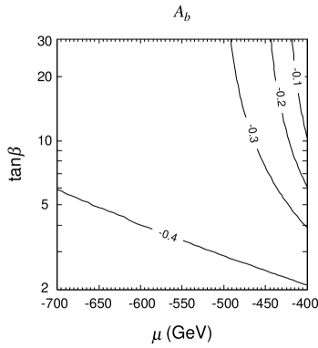
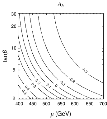
In Fig. 5, we plot contours of constant $A_{b}$ on the $\mu$ vs. $\tan\beta$ plane for $m_{\tilde{t}_{1}}=400\ {\rm GeV}$, $m_{\chi_{1}^{0}}=200\ {\rm GeV}$, and $\tan\theta_{\tilde{t}}=-0.5$. With this choice of parameters, $N_{\rm tot}\simeq 480$ for $L=100$ fb^-1 and hence we expect the experimental uncertainty of $\delta A_{b}\simeq 0.1$. Thus, quite a severe constraint may be derived on the $\mu$ vs. $\tan\beta$ plane. For negative $\mu$, regions up to $-500$ GeV is sensitive to $A_{b}$ measurements at a linear collider. While for positive $\mu$, the $\mu$ dependence becomes stronger in much wider region. Especially for a fixed value of $\tan\beta$, the $\mu$-parameter may be determined with an accuracy of $\delta\mu\sim 20\ {\rm GeV}$.

Figure 5: Contour plot of $A_{b}$ on the $\mu$ vs. $\tan\beta$ plane for Bino LSP case with $\tan\theta_{\tilde{t}}=-0.5$. Stop and LSP masses are taken to be $m_{\tilde{t}_{1}}=400$ GeV and $m_{\chi_{1}^{0}}=200$ GeV, respectively. $M_{2}$ is taken to be $500\ {\rm GeV}$.

6.2 Wino-like LSP

If the LSP is the Wino-like neutralino, a similar analysis is possible. Of course, in the Wino-like LSP case, the lightest chargino is almost degenerate with the LSP and hence the stop may also decay into the chargino and the bottom quark. The mass splitting between $\chi^{\pm}_{1}$ and $\chi^{0}_{1}$ is expected to be $O(100\ {\rm MeV})$ to a few GeV [18, 21] and hence $\chi^{\pm}_{1}$ decays into $\chi^{0}_{1}$ and soft lepton(s) or (light) meson(s). Thus, it is possible to distinguish the stop event with $\tilde{t}_{1}\rightarrow t\chi^{0}_{1}$ and that with $\tilde{t}_{1}\rightarrow b\chi^{\pm}_{1}$. In addition, we calculated the branching ratio going into top and the LSP, and found that $Br(\tilde{t}_{1}\rightarrow t\chi^{0}_{1})$ becomes $O(0.1)$ in a large parameter space. Thus, even if we cannot use all of the stop events, it is still possible to do the same analysis as before.

Figure 6: $A_{b}$ as a function of $\mu$-parameter for $\tan\theta_{\tilde{t}}=-4$ (thick line), $-2$ (dashed line), $0$ (dash-dotted line), $2$ (dotted line), and $4$ (solid line). We take $\tan\beta=10$, $m_{\tilde{t}_{1}}=400$ GeV, $m_{\chi_{1}^{0}}=200$ GeV, and $M_{1}=$ 500 GeV.

In Wino-like LSP scenario, the neutralino mixing matrix elements are approximately given by $[U_{\chi^{0}}]_{1\tilde{W}}\simeq 1$, $[U_{\chi^{0}}]_{1\tilde{B}}\simeq 0$,

$$[U_{\chi^{0}}]_{1\tilde{H}_{1}}\simeq\frac{m_{Z}\cos\theta_{W}(M_{2}\cos\beta+\mu\sin\beta)}{\mu^{2}-M_{2}^{2}},$$ (44)

and

$$[U_{\chi^{0}}]_{1\tilde{H}_{2}}\simeq-\frac{m_{Z}\cos\theta_{W}(M_{2}\sin\beta+\mu\cos\beta)}{\mu^{2}-M_{2}^{2}}.$$ (45)

Similarly to the Bino-LSP case, contamination of the Higgsino component in the LSP also induces $\mu$ dependence of $A_{b}$. The ratio $f_{L}/f_{R}$ is now given by

$$\frac{f_{L}}{f_{R}}\simeq-\frac{1}{\sqrt{2}}\frac{g_{2}}{y_{t}[U_{\chi^{0}}]_{1H_{2}}}+\tan\theta_{\tilde{t}}.$$ (46)

Since $[U_{\chi^{0}}]_{1\tilde{H}_{2}}$ is usually small and negative (we have adopted the convention that $M_{2}>0$), the relation $f_{L}/f_{R}\sim 1$ requires a negative $\tan\theta_{\tilde{t}}$ with $|\tan\theta_{\tilde{t}}|\gg 1$. This is shown in Fig. 6, where we plot $A_{b}$ as a function of $\mu$-parameter for the Wino-like LSP case. The parameters are chosen to be $\tan\beta=10$, $m_{\tilde{t}_{1}}=400$ GeV, $m_{\chi_{1}^{0}}=200$ GeV, and $M_{1}=$ 500 GeV. $A_{b}$ becomes sensitive to the $\mu$-parameter for $\tan\theta_{\tilde{t}}\sim-4$. For smaller values of negative $\tan\theta_{\tilde{t}}$, the curve shifts to the right (left) for $\mu>0$ ($\mu<0$). Such a behavior can be explained by using Eq. (45); a larger value of $|\mu|$ is needed to compensate smaller value of (negative) $\tan\theta_{\tilde{t}}$. The different behaviors for the positive and negative $\mu$ cases are due to the same reason as explained in the Bino-like LSP case. The dependence on $M_{1}$ is rather weak for large values of $M_{1}$.

Figure 7: Contour plot of $A_{b}$ on the $\mu$ vs. $\tan\beta$ plane for Wino LSP case with $\tan\theta_{\tilde{t}}=-4$. Stop and LSP masses are taken to be $m_{\tilde{t}_{1}}=400$ GeV and $m_{\chi_{1}^{0}}=200$ GeV, respectively. $M_{1}$ is taken to be 500 GeV.

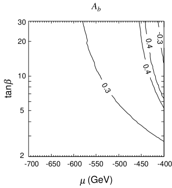
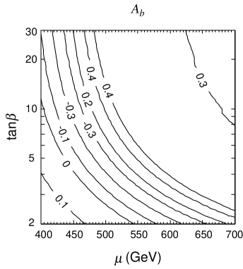
In Fig. 7, we plot the contours of constant $A_{b}$ on the $\mu$ vs. $\tan\beta$ plane for the Wino-like LSP case with $\tan\theta_{\tilde{t}}=-4$. The constraint on $\mu$ and $\tan\beta$ from the $A_{b}$ measurement is obtained in the same way as the Bino LSP case but the statistical error of $A_{b}$ depends on the branching ratio $Br(\tilde{t}_{1}\to t\chi_{1}^{0})$ since $\delta A_{b}\propto 1/\sqrt{Br(\tilde{t}_{1}\to t\chi_{1}^{0})}$. Although the number of events is reduced, we still have a possibility of constraining the values of $\mu$ and $\tan\beta$ as one can see in Fig. 7. Interestingly, very steep dependence on $\mu$ is realized in some parameter region, as shown in Fig. 7.

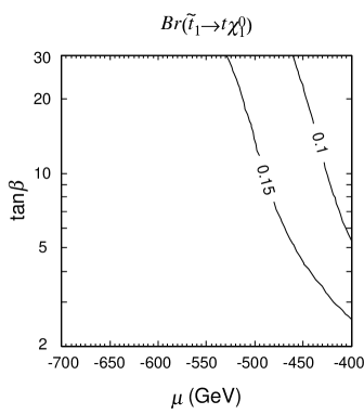
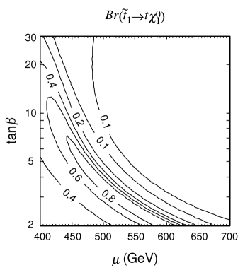
One should also note that we can use the branching ratio $Br(\tilde{t}_{1}\to t\chi_{1}^{0})$ as another observable in the Wino LSP case. In Fig. 8, we plot the contours of $Br(\tilde{t}_{1}\to t\chi_{1}^{0})$ on the $\mu$ vs. $\tan\beta$ plane for $\tan\theta_{\tilde{t}}=-4$. As one can see, $Br(\tilde{t}_{1}\to t\chi_{1}^{0})$ has sizable dependence on $\mu$ and $\tan\beta$, so that independent information on these parameters can be obtained.

Figure 8: $Br(\tilde{t}_{1}\to t\chi_{1}^{0})$ on the $\mu$ vs. $\tan\beta$ plane for Wino LSP case with $\tan\theta_{\tilde{t}}=-4$. Stop and LSP masses are taken to be $m_{\tilde{t}_{1}}=400$ GeV and $m_{\chi_{1}^{0}}=200$ GeV, respectively, and $M_{1}$ is taken to be 500 GeV.

6.3 Higgsino-like LSP

Finally we comment on the Higgsino-like LSP case. In this case, $f_{L}$ and $f_{R}$ are both dominated by the top-Yukawa contribution and hence the ratio $f_{L}/f_{R}$ becomes $\sim\tan\theta_{\tilde{t}}$. In this case, $A_{b}$ is insensitive to the gaugino masses and it is difficult to derive a constraint on $M_{1}$ and $M_{2}$. In the Higgsino-like LSP case, however, mass splitting between $\chi^{0}_{1}$ and $\chi^{\pm}_{1}$ is typically $\sim 10$ GeV or larger [22] and hence direct studies of the chargino will be possible. In addition, the second lightest neutralino is also quite degenerate with $\chi^{0}_{1}$ and hence is likely to be kinematically accessible. Thus, in this case, rather than studying the production and the decay of $\tilde{t}_{1}$, one should better study the productions and decays of $\chi^{\pm}_{1}$ and $\chi^{0}_{2}$ to understand the properties of the neutralinos and charginos [23].

7 Conclusions

We have studied the lightest stop pair production and the stop decay mode of $\tilde{t}_{1}\to t\chi_{1}^{0}$, followed by $t\to bW$ at future $e^{+}e^{-}$ linear colliders. From the naturalness point of view, stop should not be very heavy since it has a strong Yukawa interaction with the Higgs particle. Large top Yukawa coupling constant also makes one of the stop mass eigenstates light through left-right mixing in the stop mass matrix. Therefore it is reasonable to expect that linear colliders can produce the lightest stops in pair directly. If so, due to the large top Yukawa coupling constant, rich information on the model parameters is obtained by the analysis of the stop production and decay processes.

We discuss that information on $m_{\tilde{t}_{1}}$, $\theta_{\tilde{t}}$ and $m_{\chi_{1}^{0}}$ can be obtained through the measurement of the lightest stop pair production cross section using polarized electron beam and by studying the end-point energy of the top quark. We also show that the analysis of the angular distribution of the $b$-jets is useful to extract information on the neutralino sector such as neutralino mixing. We found a parameter region where it is possible to give a strong constraint on a combination of the $\mu$-parameter and $\tan\beta$ assuming $\theta_{\tilde{t}}$, $m_{\tilde{t}_{1}}$, and $m_{\chi^{0}_{1}}$ are known. Even if we cannot obtain a strong constraint on $\mu$ or $\tan\beta$, the analysis of $A_{b}$ is important since the value of $f_{L}/f_{R}$ varies depending on what the LSP is. For example, let us consider the case where there is no chargino with a nearly degenerated mass with the LSP. In such a case, one might naively expect that the LSP is Bino-like. The stop analysis we proposed provides independent information on the properties of the LSP. Such a test is significant since the value of $A_{b}$ may deviate from that in the Bino-LSP case if there is an extra neutralino such as the superpartner of the singlet Higgs boson.