IFIC/02-38
UWThPh-2002-25
Constraining Majorana neutrino electromagnetic properties from the LMA-MSW solution of the solar neutrino problem

Abstract

In this paper we use solar neutrino data to derive stringent bounds on Majorana neutrino transition moments (TMs). Should such be present, they would contribute to the neutrino–electron scattering cross section and hence alter the signal observed in Super-Kamiokande. Motivated by the growing robustness of the LMA-MSW solution of the solar neutrino problem indicated by recent data, and also by the prospects of its possible confirmation at KamLAND, we assume the validity of this solution, and we constrain neutrino TMs by using the latest global solar neutrino data. We find that all elements of the TM matrix can be bounded at the same time. Furthermore, we show how reactor data play a complementary role to the solar neutrino data, and use the combination of both data sets to improve the current bounds. Performing a simultaneous fit of LMA-MSW oscillation parameters and TMs we find that $6.3\times 10^{-10}\mu_{B}$ and $2.0\times 10^{-10}\mu_{B}$ are the 90% C.L. bounds from solar and combined solar + reactor data, respectively. Finally, we perform a simulation of the upcoming Borexino experiment and show that it will improve the bounds from today’s data by roughly one order of magnitude.

1 Introduction

Present solar Cleveland:nv , Abdurashitov:2002nt , GaGNO , Fukuda:2002pe , SNONC , SNODN and atmospheric neutrino data atm02 , Fukuda:1998mi provide the first robust evidence for neutrino flavour conversion and, consequently, the first solid indication for new physics. Neutrino oscillations constitute the most popular explanation for the data (for recent analyses see Refs. Maltoni:2002ni , solfits , 3flavors ) and are a natural outcome of gauge theories of neutrino mass Schechter:1980gr , rev . Non-zero neutrino masses manifest themselves through non-standard neutrino electromagnetic properties. If the lepton sector in the Standard Model (SM) were minimally extended in analogy with the quark sector, neutrinos get Dirac masses ($m_{\nu}$) and their magnetic moments (MMs) are tiny Fujikawa:yx ,

$$\mu_{\nu}\simeq 3\times 10^{-19}\mu_{B}\left(\frac{m_{\nu}}{1\,\mathrm{eV}}\right)\,,$$ (1)

where $\mu_{B}$ is the Bohr magneton. Laboratory experiments give 90% C.L. bounds on the neutrino MMs of $1.8\times 10^{-10}\mu_{B}$ Derbin:wy , Derbin:ua and $1.3\times 10^{-10}\mu_{B}$ munu for the electron neutrino, $6.8\times 10^{-10}\mu_{B}$ for the muon neutrino LSND and $3.9\times 10^{-7}\mu_{B}$ for the tau neutrino DONUT (see also Ref. Hagiwara:pw ). On the other hand, astrophysics and cosmology provide limits of the order of $10^{-12}$ to $10^{-11}$ Bohr magnetons Raffelt:gv . Improved sensitivity for the electron neutrino MM from reactor neutrino experiments is expected, while a tritium $\bar{\nu}_{e}$ source experiment H3 aims to reach $3\times 10^{-12}\mu_{B}$.

It has for a long time been noticed, on quite general “naturality” grounds, that Majorana neutrinos constitute the typical outcome of gauge theories Schechter:1980gr . On the other hand, precisely such neutrinos also emerge in specific classes of unified theories, in particular, in those employing the seesaw mechanism rev . If neutrinos are indeed Majorana particles the structure of their electromagnetic properties differs crucially from that of Dirac neutrinos Schechter:1981hw , being characterized by a $3\times 3$ complex antisymmetric matrix $\lambda$, the so-called Majorana transition moment (TM) matrix. It contains MMs as well as electric dipole moments of the neutrinos. The existence of any electromagnetic neutrino moment well above the expectation in Eq. (1) would signal that some special mechanism—which goes beyond the SM—is at work. Therefore, neutrino electromagnetic properties are interesting probes of new physics.

As noted in Ref. Schechter:1981hw the existence of Majorana transition moments leads to the phenomenon of spin-flavour precession, when they move through a magnetic field, as might happen in the Sun. This was subsequently shown to affect the propagation of solar neutrinos in an important way, due to the effects of matter Akhmedov:uk , and this has recently been shown to provide excellent fits to current data Miranda .

In the present paper we will take a different attitude. Motivated by the now robust status of the LMA-MSW solution of the solar neutrino problem indicated by recent data Maltoni:2002ni , solfits , and also by the prospects of its possible confirmation by the KamLAND experiment kamland , we take up this solution as the basis of our investigation. It has been shown in Ref. Miranda that in this case the effect of a solar magnetic field can be safely neglected. Therefore, our present approach is justified and complementary to that in Ref. Miranda : there we were concerned with spin-flavour-conversions of solar neutrinos, sensitive to the product of $\lambda$ times a solar magnetic field, while here we are concerned with the effect of TMs in the neutrino detection process. Sizable TMs would contribute to the elastic neutrino–electron scattering in the Super-Kamiokande (SK) experiment Fukuda:2002pe , and hence, data from this experiment can be used to constrain electromagnetic neutrino properties Beacom:1999wx , joshipura .

Here we will tacitly employ the results of the latest analysis in Ref. Maltoni:2002ni as well as the fit strategies used there, to perform a fit to the global solar neutrino data in terms of LMA-MSW oscillation parameters and neutrino TMs, in order to derive bounds on the latter. It is important to clarify for which combinations of the three complex moments the bounds are valid. We will show that all three moments can be bounded, however, not all at the same level. In addition, we will show that data from reactor neutrino experiments Derbin:wy , Derbin:ua , munu which use elastic neutrino–electron scattering for neutrino detection are to some extent complementary to the solar neutrino data, so that by combining both data sets one can improve the bounds. We also explore the potential of the upcoming Borexino experiment borexino , Alimonti:2002xc in probing the TMs, showing that it is substantially more sensitive to the TMs than present experiments.

The paper is organized as follows. In Section 2 we give our theoretical framework and we discuss in detail which elements of the TM matrix are constrained. In Section 3 we present the statistical method we apply to calculate bounds on the TMs, and in Section 4 we describe our analysis of solar and reactor neutrino data. The resulting bounds are discussed in Section 5 and the sensitivity of the upcoming Borexino experiment is considered in Section 6. A brief discussion concludes the paper in Section 7.

2 The theoretical framework

In this paper, we adopt the following basic working assumptions:

• Only three light neutrinos exist, doublets under $SU(2)\otimes U(1)$ (no light sterile neutrinos); this is well-motivated by recent global fits of all available neutrino oscillation data, including also those that follow from short baseline searches Maltoni:2002xd .

• The solution of the solar neutrino puzzle is given by the LMA-MSW solution, as indicated by recent global fits of solar data solfits , 3flavors .

• Neutrinos have Majorana nature as expected from theory rev , Schechter:1981hw .

• Neutrinos are endowed with TMs arising from some unspecified electroweak gauge theory.

Although the latter is probably the least motivated of our assumptions, there are some models of the electroweak interaction where the possibility of enhanced TMs has been discussed rev .

In experiments where the neutrino detection reaction is elastic neutrino–electron scattering, like in SK, Borexino and some reactor experiments Derbin:wy , Derbin:ua , munu , the electromagnetic cross section is Bardin:wr

$$\frac{d\sigma_{\mathrm{em}}}{dT}=\frac{\alpha^{2}\pi}{m_{e}^{2}\mu_{B}^{2}}\left(\frac{1}{T}-\frac{1}{E_{\nu}}\right)\mu^{2}_{\mathrm{eff}}\,,$$ (2)

where the effective MM square is given by GS

$$\mu^{2}_{\mathrm{eff}}=a_{-}^{\dagger}\lambda^{\dagger}\lambda a_{-}+a_{+}^{\dagger}\lambda\lambda^{\dagger}a_{+}\,.$$ (3)

The electromagnetic cross section adds to the weak cross section and allows to extract information on the TM matrix $\lambda$. In this cross section, $T$ denotes the kinetic energy of the recoil electron, $E_{\nu}$ is the energy of the incoming neutrino and the 3-vectors $a_{-}$ and $a_{+}$ denote the neutrino amplitudes for negative and positive helicities, respectively, at the detector. The square of the effective MM given in Eq. (3) is independent of the basis chosen for the neutrino state GS . In what follows we consider both the flavour basis and the mass eigenstate basis. We will use the convention that $a_{\mp}$ and $\lambda=(\lambda_{\alpha\beta})$ denote the quantities in the flavour basis, whereas in the mass basis we will use $\tilde{a}_{\mp}$ and $\tilde{\lambda}=(\lambda_{jk})$. The two bases are connected via the neutrino mixing matrix $U$:

$$\tilde{a}_{-}=U^{\dagger}a_{-}\,,\quad\tilde{a}_{+}=U^{T}a_{+}\,,\quad\tilde{\lambda}=U^{T}\lambda U\,.$$ (4)

One usually decomposes the transition moment matrix as

$$\lambda=\mu-id\,,$$ (5)

where $\mu$ and $d$ are hermitian matrices. On general grounds these matrices are, in addition, antisymmetric and imaginary for Majorana neutrinos Schechter:1981hw (see also Ref. GS and references cited therein). It is, furthermore, useful to define vectors $\mathbf{\Lambda}=(\Lambda_{\alpha})$ and $\tilde{\mathbf{\Lambda}}=(\Lambda_{j})$ in the flavour and mass basis, respectively, by

$$\lambda_{\alpha\beta}=\varepsilon_{\alpha\beta\gamma}\Lambda_{\gamma}\quad\mathrm{and}\quad\lambda_{jk}=\varepsilon_{jkl}\Lambda_{l}\,.$$ (6)

Thus, in the flavour basis we have $\lambda_{e\mu}=\Lambda_{\tau}$, $\lambda_{\mu\tau}=\Lambda_{e}$ and $\lambda_{\tau e}=\Lambda_{\mu}$. Note also that

$$|\mathbf{\Lambda}|^{2}=\frac{1}{2}\,\mathrm{Tr}\left(\lambda^{\dagger}\lambda\right)\quad\Rightarrow\quad|\mathbf{\Lambda}|=|\tilde{\mathbf{\Lambda}}|\,.$$ (7)

This means if we are able to find a bound on $|\mathbf{\Lambda}|$, we have not only constrained the TMs in the flavour basis but also in the mass basis. In the numerical section of the paper, this will be exactly our strategy.

Let us now discuss the detailed form that the effective MM square $\mu_{\mathrm{eff}}^{2}$ in Eq. (3) takes when we assume the LMA-MSW solution of the solar neutrino problem, denoted by $\mu_{\mathrm{LMA}}^{2}$. Numerical integrations of the neutrino evolution equations performed in Ref. Miranda showed that for an effective MM of $10^{-11}\mu_{B}$ a solar magnetic field of the order of 80 KGauss has practically no effect on the LMA-MSW solution. The results of Ref. Miranda imply that it is safe to neglect possible solar magnetic field effects on the evolution of the neutrino state in the sun in case of LMA-MSW. This follows essentially from the fact that the terms in the evolution Hamiltonian related to the LMA-MSW mass-squared difference and the matter potential are much bigger than the electromagnetic terms. Hence, helicity is conserved in solar neutrino propagation, so that we can set $a_{+}=0$, thereby eliminating the second term in Eq. (3). Another good approximation used in fitting solar data in a three-neutrino scenario 3flavors is to set $\Delta m^{2}{atm}\gg\Delta m^{2}{sol}\equiv\Delta m^{2}$, i.e., oscillations with $\Delta m^{2}{atm}$ are averaged out. Using the parameterization (6) we obtain from Eq. (3)

$$\mu^{2}_{\mathrm{LMA}}=|\mathbf{\Lambda}|^{2}-P^{3\nu}_{e3}|\Lambda_{3}|^{2}-\sum_{j,k=1}^{2}\left\langle(\tilde{a}^{j}_{-})(\tilde{a}^{k}_{-})^{*}\right\rangle\Lambda_{j}^{*}\Lambda_{k}\,.$$ (8)

The brackets $\left\langle...\right\rangle$ in the last term in Eq. (8) denote the average over the production point, earth-sun distance and zenith angle, and we have made use of the relation

$$P^{3\nu}_{ej}\equiv\left\langle|\tilde{a}_{-}^{j}|^{2}\right\rangle\quad(j=1,2,3)$$ (9)

for the probability that the neutrino produced in the core of the sun as a $\nu_{e}$ arrives at the detector as a mass eigenstate $\nu_{j}$. From Eq. (8) one learns that besides the absolute values of the TMs $|\Lambda_{1}|,|\Lambda_{2}|,|\Lambda_{3}|$ only one complex phase $\delta=\mathrm{arg}(\Lambda_{1}^{*}\Lambda_{2})$ enters into $\mu^{2}_{\mathrm{LMA}}$.

Eq. (8) can be further simplified by making use of the large mass-squared difference $\Delta m^{2}\sim 5\times 10^{-5}$ eV² implied by the LMA-MSW solution. First, because of vacuum oscillations on the way from the sun to the earth the neutrino state arriving at the earth can be considered as an incoherent mixture of mass eigenstates GS , dighe . Note also that for the LMA-MSW solution, earth matter effects are very small earthmatter so that we neglect them in our expression for $\mu^{2}_{\mathrm{LMA}}$. Then we find that only the diagonal elements of the matrix $\left({\tilde{\lambda}}^{\dagger}\tilde{\lambda}\right)$ contribute, and as a result only the probabilities (9) appear in determining the detected neutrino signal. Setting $s_{13}\equiv\sin\theta_{13}$, $c_{13}\equiv\cos\theta_{13}$ and $U_{e3}=s_{13}$ one has, to a very good approximation 3flavors ,

$$P^{3\nu}_{e3}=s_{13}^{2}\quad\mathrm{and}\quad P^{3\nu}_{ej}=c_{13}^{2}P^{2\nu}_{ej}\;(j=1,2)\quad\mathrm{with}\quad P^{2\nu}_{e1}+P^{2\nu}_{e2}=1\,.$$ (10)

The probabilities $P^{2\nu}_{ej}$ $(j=1,2)$ are the effective 2-neutrino probabilities for the solar neutrino problem, where all the averages mentioned above have been taken into account. Using now the probabilities in Eq. (10) and the approximations mentioned above, Eq. (8) becomes

$$\mu^{2}_{\mathrm{LMA}}=|\Lambda_{1}|^{2}+|\Lambda_{2}|^{2}+c_{13}^{2}|\Lambda_{3}|^{2}-c_{13}^{2}\sum_{j=1,2}P^{2\nu}_{ej}|\Lambda_{j}|^{2}\,.$$ (11)

It is well known from reactor neutrino data CHOOZ that the mixing angle $\theta_{13}$ is rather small. Fits to the CHOOZ data and atmospheric neutrino data 3flavors show that at 3$\sigma$ one has $s_{13}^{2}\>\mbox{\raisebox{-3.0pt}{$\stackrel{{\scriptstyle\displaystyle<}}{{\sim}}$}}\>0.05$. This allows us to replace $c_{13}^{2}$ in Eq. (11) by 1. Then we arrive at the final formula

$$\mu^{2}_{\mathrm{LMA}}=|\mathbf{\Lambda}|^{2}-|\Lambda_{2}|^{2}+P^{2\nu}_{e1}\left(|\Lambda_{2}|^{2}-|\Lambda_{1}|^{2}\right)\,,$$ (12)

which will be used in the numerical section evaluating solar neutrino data. The probability $P^{2\nu}_{e1}$ is a function of the ratio $\Delta m^{2}/E_{\nu}$ and the solar mixing angle $\theta\equiv\theta_{12}$. In the following we will drop the super-script $2\nu$ and $P_{e1}$ or $P_{ee}$ refers always to a 2-neutrino probability. Eq. (12) naturally makes no distinction between MMs and electric dipole moments. Since we aim at constraining $|\mathbf{\Lambda}|$, all elements of the TM matrix will be bounded at the same time.

Now we move to the case of reactor neutrinos. There we have a pure $\bar{\nu}_{e}$ source. Therefore, we have $a_{-}=0$ and $a_{+}=(1,0,0)^{T}$ since in these experiments the baseline is much too short for any oscillations to develop. The resulting $\mu_{\mathrm{eff}}^{2}$ relevant in reactor experiments is given as

$$\mu_{\mathrm{R}}^{2}=|\Lambda_{\mu}|^{2}+|\Lambda_{\tau}|^{2}\,.$$ (13)

From this relation it is clear that reactor data on its own cannot constrain all TMs contained in $\lambda$, since $\Lambda_{e}$ does not enter in Eq. (13). In order to combine reactor and solar data it is useful to rewrite $\mu_{\mathrm{R}}^{2}$ in terms of the mass basis quantities. With Eq. (6) we readily derive

$$\left(\tilde{\lambda}{\tilde{\lambda}}^{\dagger}\right)_{jk}=|\mathbf{\Lambda}|^{2}\delta_{jk}-\Lambda_{j}\Lambda_{k}^{*}\,.$$ (14)

Then with Eq. (4) we obtain

$$\mu_{\mathrm{R}}^{2}=|\mathbf{\Lambda}|^{2}-c^{2}|\Lambda_{1}|^{2}-s^{2}|\Lambda_{2}|^{2}-2sc|\Lambda_{1}||\Lambda_{2}|\cos\delta\,,$$ (15)

where $c=\cos\theta$ and $s=\sin\theta$, $\theta$ being the solar mixing angle. Further, we notice that the relative phase $\delta=\mathrm{arg}(\Lambda_{1}^{*}\Lambda_{2})$ between $\Lambda_{1}$ and $\Lambda_{2}$ appears in addition to $|\mathbf{\Lambda}|$, $|\Lambda_{1}|$ and $|\Lambda_{2}|$.

3 Statistical method and qualitative discussion

In the following we will use data from solar and reactor neutrino experiments to constrain neutrino TMs. The $\chi^{2}$-function obtained from the data depends on the solar oscillation parameters $\tan^{2}\theta$ and $\Delta m^{2}$ as well as on the elements of the TM matrix $\lambda$. Regarding the dependence on the oscillation parameters we will take two different attitudes. One is to assume that $\tan^{2}\theta$ and $\Delta m^{2}$ will be determined with good accuracy at the KamLAND experiment, and hence, we will consider the $\chi^{2}$ at fixed points in the $\tan^{2}\theta-\Delta m^{2}$ plane (method I). In the second approach we will derive a bound on the TMs by minimizing the $\chi^{2}$ with respect to $\tan^{2}\theta$ and $\Delta m^{2}$ (method II). This second procedure takes into account the present uncertainty of our knowledge of the oscillation parameters.

Let us describe in detail how we calculate a bound on the TMs. Our aim is to constrain $|\mathbf{\Lambda}|$, therefore it is convenient to consider the $\chi^{2}$ as a function of the independent parameters $|\mathbf{\Lambda}|,|\Lambda_{1}|,|\Lambda_{2}|$ and $\delta$. As discussed in the previous section, $\delta$ appears only if reactor data are included. The $\chi^{2}$-functions which we are using for the individual data sets (solar rates, SK recoil electron spectrum, reactor data) will be described in detail in the following sections. When performing the fit to the data, we find that in general the minimum of the $\chi^{2}$ occurs close or outside the physical boundary of the parameters $|\mathbf{\Lambda}|,|\Lambda_{1}|,|\Lambda_{2}|$. To take this into account we apply Bayesian techniques to calculate an upper bound on $|\mathbf{\Lambda}|$. We minimize the $\chi^{2}$ with respect to $|\Lambda_{1}|$, $|\Lambda_{2}|$ and $\delta$ for each value of $|\mathbf{\Lambda}|$, taking into account the allowed region $0\leq|\Lambda_{1}|^{2}+|\Lambda_{2}|^{2}\leq|\mathbf{\Lambda}|^{2}$:

$$\chi^{2}(|\mathbf{\Lambda}|)=\mathrm{Min}\left[\chi^{2}(|\mathbf{\Lambda}|,|\Lambda_{1}|,|\Lambda_{2}|,\delta)\right]\,.$$ (16)

In method I we do this for fixed values of the oscillation parameters, scanning over the LMA-MSW region, whereas in method II we minimize also with respect to $\tan^{2}\theta$ and $\Delta m^{2}$ in Eq. (16). Then the $\chi^{2}$ is transformed into a likelihood function via

$$\mathcal{L}\propto\exp\left(-\frac{1}{2}\chi^{2}\right)\,.$$ (17)

Now we use Bayes’ theorem and a flat prior distribution $p(|\mathbf{\Lambda}|)$ in the physically allowed region, $p(|\mathbf{\Lambda}|)=\Theta(|\mathbf{\Lambda}|)$, to obtain a probability distribution for $|\mathbf{\Lambda}|$:

$$f(|\mathbf{\Lambda}|)\,d|\mathbf{\Lambda}|=\frac{\mathcal{L}(|\mathbf{\Lambda}|)\,\Theta(|\mathbf{\Lambda}|)\,d|\mathbf{\Lambda}|}{\int_{0}^{\infty}\mathcal{L}(|\mathbf{\Lambda}|^{\prime})\,d|\mathbf{\Lambda}|^{\prime}}\,.$$ (18)

An upper bound $b_{\alpha}$ on $|\mathbf{\Lambda}|$ at a C.L. $\alpha$ is given by the equation

$$\int_{0}^{b_{\alpha}}f(|\mathbf{\Lambda}|)d|\mathbf{\Lambda}|=\alpha\,.$$ (19)

Let us consider in more detail the minimization with respect to $|\Lambda_{1}|$ and $|\Lambda_{2}|$ in Eq. (16) in the case of solar data without reactor. As we will show later there is no evidence for a non-zero $\mu_{\mathrm{LMA}}^{2}$ in the data. Therefore the minimum of the $\chi^{2}$ for a given $|\mathbf{\Lambda}|$ will occur if $\mu_{\mathrm{LMA}}^{2}$ is minimal. Departing from Eq. (12) it is easy to show that

$$\mathrm{Min}\,[\mu^{2}_{\mathrm{LMA}}]=\left\{\begin{array}[]{l@{\quad}l}|\mathbf{\Lambda}|^{2}\,P_{e1}&\mathrm{for}\quad P_{e1}\leq 0.5\,,\\ |\mathbf{\Lambda}|^{2}\,(1-P_{e1})&\mathrm{for}\quad P_{e1}>0.5\,.\end{array}\right.$$ (20)

The minimum occurs at

$$|\mathbf{\Lambda}|^{2}=\left\{\begin{array}[]{l@{\quad\mbox{for}\quad}l}|\Lambda_{2}|^{2}&P_{e1}<0.5\,,\\ |\Lambda_{1}|^{2}+|\Lambda_{2}|^{2}&P_{e1}=0.5\,,\\ |\Lambda_{1}|^{2}&P_{e1}>0.5\,.\end{array}\right.$$ (21)

From Eq. (20) follows that the bound on $|\mathbf{\Lambda}|$ is strongest if $P_{e1}=0.5$ because in this situation $\mu_{\mathrm{LMA}}^{2}$ is maximal. In Fig. 1 we show contours of constant $P_{e1}$ in the $\tan^{2}\theta-\Delta m^{2}/E_{\nu}$ plane. For definiteness, the probabilities in the figure are obtained by performing the averaging over the production distribution inside the sun for the ⁷Be flux most relevant for Borexino. However, the probabilities for the ⁸B flux relevant for SK are very similar.

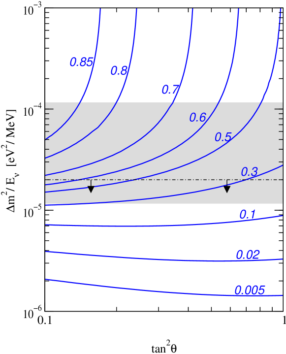
Figure 1: Contours of constant $P_{e1}$. The shaded region is relevant for Borexino, whereas the region below the dash-dotted line is relevant for SK.

The shaded region in Fig. 1 is the region relevant for Borexino, assuming a mass-squared difference in the range $10^{-5}$ eV${}^{2}<\Delta m^{2}<10^{-4}$ eV², whereas for SK the region below the dash-dotted line is most important, due to the higher energy of the ⁸B neutrinos. We can read off from the figure that in most part of the SK region $P_{e1}$ is very small. According to Eq. (21) this means that the sensitivity of SK for $|\mathbf{\Lambda}|$ is limited because of the small $P_{e1}$. In contrast, we expect a much better sensitivity of Borexino, because, in a large part of the relevant parameter space in this case, $P_{e1}$ is close to the optimal value of $0.5$.

The arguments presented here are valid as long as the $\chi^{2}$ depends only on the parameter combination given in Eq. (12). The data from reactor experiments depend on a different combination of TM parameters (see Eq. (15)) implying that the combined analysis of SK and reactor data will potentially lead to more stringent limits than the SK data alone.

4 Analysis of solar and reactor neutrino data

In this section we describe briefly our analysis of solar neutrino data and the data which we are using from reactor neutrino experiments. Neglecting the electromagnetic contribution to the small elastic scattering signal in SNO, one notices that the neutrino TMs contribute directly to the observed signal only in SK. However, the uncertainty in the ⁸B flux leads to correlations between SK and all other experiments. Therefore, even for fixed oscillation parameters (method I), also other experiments give some information on TMs and it is important to include them in the analysis joshipura .

We divide the solar neutrino data into the total rates observed in all experiments and the SK recoil electron spectrum (with free overall normalization). Before combining rates with SK spectra, we derive bounds on $|\mathbf{\Lambda}|$ for each of these cases separately. Subsequently we consider the reactor data by themselves and in combination with the global sample of solar data.

4.1 Solar rates

In this analysis we use the event rates measured in the Chlorine experiment Homestake Cleveland:nv (Cl), the Gallium experiments Sage Abdurashitov:2002nt , Gallex and GNO GaGNO (GaGNO), the total event rate of SK Fukuda:2002pe based on the 1496 days data sample and the recent result of the Sudbury neutrino observatory SNONC for the charged current (SNO CC) and neutral current (SNO NC) solar neutrino rates. For the analysis we use the $\chi^{2}$-function

$$\chi^{2}_{\mathrm{rates}}=\sum_{j,k}(R_{j}-D_{j})(V^{\mathrm{rate}}_{jk})^{-1}(R_{k}-D_{k})\,.$$ (22)

Here the indices $j,k$ run over the 6 solar neutrino rates (Cl, Sage, GaGNO, SK, SNO CC, SNO NC), $D_{j}$ are the experimental rates, $R_{j}$ are the theoretical predictions and $V^{\mathrm{rate}}_{jk}$ is the covariance matrix.

Cl Cleveland:nv	$2.56\pm 0.16\pm 0.16$ SNU
Sage Abdurashitov:2002nt	$70.8\,{{}^{+5.3}_{-5.2}}\,{{}^{+3.7}_{-3.2}}$ SNU
GaGNO GaGNO	$73.3\pm 4.7\pm 4.0$ SNU
SK Fukuda:2002pe	$0.465\pm 0.005\,{{}^{+0.014}_{-0.012}}$
SNO CC SNONC	$0.3485\pm 0.012\pm 0.018$
SNO NC SNONC	$1.008\pm 0.087\pm 0.097$

Table 1: Solar neutrino rates used in our analysis. For SK and SNO the given number is the ratio of the observed flux and the ⁸B flux predicted by the BP00 SSM BP00 .

The data we are using are given in Table 1. The rates of SK and SNO are the ratio of the measured flux and the ⁸B flux predicted by the standard solar model (SSM) BP00 BP00 and no disappearance of solar $\nu_{e}$ ($\Phi^{0}_{\mathrm{B}}=5.05\times 10^{6}$ cm^-2s^-1). Note that the SNO CC and NC fluxes as given in Ref. SNONC have been obtained from a fit to the SNO spectral data assuming no distortion of the neutrino energy spectrum, i.e., a survival probability constant in energy, which in general is not realized in the case of neutrino oscillations. However, in the case of the LMA-MSW solution it is a very good approximation to use the fluxes given in Ref. SNONC .

The theoretical predictions $R_{j}$ which appear in Eq. (22) are calculated as described in Ref. Maltoni:2002ni . However, the rate $R_{\mathrm{SK}}$ of the SK experiment includes an extra contribution from the electromagnetic scattering. This rate is given by

$$R_{\mathrm{SK}}=\frac{\int_{0}^{\infty}dE_{\nu}\,\phi_{\mathrm{B}}(E_{\nu})\left\{P_{ee}(E_{\nu})\sigma^{W}_{e}(E_{\nu})+[1-P_{ee}(E_{\nu})]\sigma^{W}_{\mu}(E_{\nu})+\mu^{2}_{\mathrm{LMA}}(E_{\nu})\sigma^{\prime}_{\mathrm{em}}(E_{\nu})\right\}}{\int_{0}^{\infty}dE_{\nu}\,\phi_{\mathrm{B}}(E_{\nu})\,\sigma^{W}_{e}(E_{\nu})}\,,$$ (23)

where $\phi_{\mathrm{B}}(E_{\nu})$ is the shape of the ⁸B flux normalized to 1, which we take from Ref. bahcallpage , and

$$\sigma(E_{\nu})=\int_{0}^{T_{\mathrm{max}}(E_{\nu})}dT^{\prime}\frac{d\sigma(T^{\prime},E_{\nu})}{dT^{\prime}}\int_{T_{1}}^{T_{2}}dT\,R(T^{\prime},T)\quad\mbox{with}\quad\sigma=\sigma^{W}_{e},\sigma^{W}_{\mu},\sigma^{\prime}_{\mathrm{em}}\,.$$ (24)

We use the SM weak cross sections $\sigma^{W}_{e,\mu}$ including radiative corrections Bahcall:1995mm , $\mu_{\mathrm{LMA}}^{2}$ is given in Eq. (12), and

$$\frac{d\sigma^{\prime}_{\mathrm{em}}(T^{\prime},E_{\nu})}{dT^{\prime}}=\frac{\alpha^{2}\pi}{m_{e}^{2}\mu_{B}^{2}}\left(\frac{1}{T^{\prime}}-\frac{1}{E_{\nu}}\right)\,.$$ (25)

Here $E_{\nu}$ is the neutrino energy, while $T^{\prime}$ and $T$ denote the true and the measured recoil electron kinetic energies, respectively. The integration in $T$ is from the SK threshold 5 MeV (total electron energy) up to 20 MeV. The maximum kinetic energy of the recoil electrons is given by $T_{\mathrm{max}}(E_{\nu})=2E_{\nu}^{2}/(2E_{\nu}+m_{e})$. The resolution function $R(T^{\prime},T)$ is taken from Ref. Fukuda:1998ua .

The covariance matrix $V^{\mathrm{rate}}_{jk}$ in the $\chi^{2}$ of Eq. (22) takes into account the experimental errors and theoretical uncertainties from detection cross sections $V_{jk}^{\mathrm{CS}}$ and SSM predictions $V_{jk}^{\mathrm{flux}}$ added in quadrature fogli ,

$$V_{jk}^{\mathrm{rate}}=V_{jk}^{\mathrm{exp}}+V_{jk}^{\mathrm{CS}}+V_{jk}^{\mathrm{flux}}\,.$$ (26)

The experimental errors for different experiments are uncorrelated. For $j,k=$ Cl, Sage, GaGNO, SK we have $V_{jk}^{\mathrm{exp}}=\delta_{jk}\sigma^{2}_{j}$, where the $\sigma^{2}_{j}$ are the experimental uncertainties, calculated by adding in quadrature the statistical and systematic uncertainties given in Table 1. However, the statistical and systematic errors for the SNO CC and NC rates are strongly correlated, with $\rho^{\mathrm{stat}}=-0.518$ (the same as the correlation for the CC and NC day-night asymmetry, given in Ref. SNODN ) and $\rho^{\mathrm{sys}}=-0.508$ (which we derive from Table II of Ref. SNONC ). The second and third terms in Eq. (26) take into account the uncertainties in the detection cross sections and in the SSM predictions of the neutrino fluxes, respectively. For details see Refs. Maltoni:2002ni , fogli and references therein.

4.2 The Super-Kamiokande recoil electron spectrum

In this section we consider the shape of the SK recoil electron spectrum. The electromagnetic contribution to the neutrino–electron scattering cross section leads to a substantially different spectrum of the scattered electrons than expected from the SM weak interaction. Therefore, the SK spectral data provide a useful tool to constrain neutrino TMs Beacom:1999wx .

We perform a fit to the latest 1496 days SK data presented in Ref. Fukuda:2002pe . There the event rates are given in 8 energy bins ranging from 5 to 20 MeV. The energy bins 2 to 7 are further divided into 7 bins of zenith angle, which makes up a total of 44 data points $D_{i}$. We define the $\chi^{2}$-function

$$\chi^{2}_{\mathrm{spect}}=\sum_{i,j=1}^{44}(\alpha R_{i}-D_{i})(V^{\mathrm{spect}}_{ij})^{-1}(\alpha R_{j}-D_{j})\,.$$ (27)

The theoretical prediction $R_{i}(\tan^{2}\theta,\Delta m^{2},\mu^{2}_{\mathrm{LMA}})$ for the $i$-th bin is calculated as in Eq. (23) with the integration interval $[T_{1},T_{2}]$ in Eq. (24) chosen according to the energy interval of the given bin. The covariance matrix $V^{\mathrm{spect}}_{ij}$ in Eq. (27) contains statistical and systematic experimental errors. These are obtained from Ref. Fukuda:2002pe taking into account the correct correlations of systematic errors. The $\chi^{2}$ of Eq. (27) is minimized with respect to the normalization factor $\alpha$ in order to isolate only the shape of the spectrum.

4.3 Reactor data

Data from neutrino electron scattering at nuclear reactor experiments Derbin:wy , Derbin:ua , munu can be used to constrain the combination of TMs given in Eq. (15). Here we use data from the Rovno nuclear power plant Derbin:wy and from the Bugey reactor munu . To include this information in our analysis we make the following ansatz for the $\chi^{2}$-function:

$$\chi^{2}_{\mathrm{reactor}}(\mu_{\mathrm{R}})=\sum_{i}\left(\frac{N^{i}_{\mathrm{weak}}+N^{i}_{\mathrm{em}}(\mu_{\mathrm{R}})-N^{i}_{\mathrm{obs}}}{\sigma^{i}}\right)^{2}\,.$$ (28)

The sum is over the two experiments Rovno and Bugey, $N^{i}_{\mathrm{obs}}$ is the observed number of events with the one standard deviation error $\sigma^{i}$, $N^{i}_{\mathrm{weak}}$ is the number of events expected in the case of no neutrino TMs (only the standard weak interaction) and $N^{i}_{\mathrm{em}}(\mu_{\mathrm{R}})$ is the number of events due to the electromagnetic scattering of neutrinos with an effective MM $\mu_{\mathrm{R}}$. We can write the latter as

$$N^{i}_{\mathrm{em}}(\mu_{\mathrm{R}})=C^{i}\,\left(\frac{\mu_{\mathrm{R}}}{10^{-10}\mu_{B}}\right)^{2}\,.$$ (29)

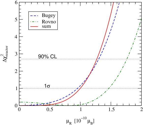
Figure 2: $\Delta\chi^{2}$ of the reactor experiments Rovno Derbin:wy and Bugey munu and the total $\Delta\chi^{2}_{\mathrm{reactor}}$ as a function of the effective MM.

For the Rovno reactor we obtain from Table I of Ref. Derbin:wy the values $N^{\mathrm{Rovno}}_{\mathrm{obs}}=41$, $\sigma^{\mathrm{Rovno}}=20$ and $N^{\mathrm{Rovno}}_{\mathrm{weak}}=32$. Furthermore, in this table the number of events due to the electromagnetic scattering of neutrinos with an effective MM $\mu_{\mathrm{R}}=2\times 10^{-10}\mu_{B}$ is given: $N^{\mathrm{Rovno}}_{\mathrm{em}}(2\times 10^{-10}\mu_{B})=54$. Using this last information the constant in Eq. (29) can be determined as $C^{\mathrm{Rovno}}=54/4$. Results of the MUNU experiment performed at the Bugey reactor have been presented recently at the Neutrino 2002 conference munu . These lead to the bound $\mu_{\mathrm{R}}<1.3\times 10^{-10}\mu_{B}$ at 90 % C.L., if an energy cut of $E_{e}>1$ MeV is used. From Ref. munu we get (in events per day) $N^{\mathrm{Bugey}}_{\mathrm{obs}}=0.37$, $\sigma^{\mathrm{Bugey}}=0.25$ and $N^{\mathrm{Bugey}}_{\mathrm{weak}}=0.45$. The constant in Eq. (29) can be calculated by making use of the 90% C.L. bound cited above: we solve the equation $\chi^{2}_{\mathrm{Bugey}}(\mu_{\mathrm{R}}=1.3\times 10^{-10}\mu_{B})=2.7$. This leads to $C^{\mathrm{Bugey}}=0.196$. In Fig. 2 we show the $\Delta\chi^{2}$ of the two experiments and also the sum. Note that with our ansatz Eqs. (28) and (29) we can reproduce to good accuracy the 1 $\sigma$ upper bound $\mu_{\mathrm{R}}<1.5\times 10^{-10}\mu_{B}$ from the Rovno data Derbin:wy .

5 Bounds on $|\mathbf{\Lambda}|$ from solar and reactor data

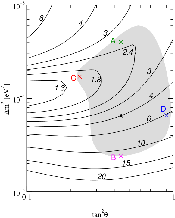
Figure 3: Contours of the 90% C.L. bound on $|\mathbf{\Lambda}|$ in units of $10^{-10}\mu_{B}$ from solar data. The shaded region is the 3$\sigma$ LMA-MSW region from Ref. Maltoni:2002ni , the best fit point is marked with a star. The crosses labeled A, B, C, D are the test points considered in Table 2.

First we discuss the bounds on $|\mathbf{\Lambda}|$ from solar data alone. Fixing the oscillation parameters at the current best fit point $\tan^{2}\theta=0.44$, $\Delta m^{2}=6.6\times 10^{-5}$ eV² Maltoni:2002ni we obtain with the Bayesian methods described in Section 3 the 90% C.L. bound

$$|\mathbf{\Lambda}|<4.0\times 10^{-10}\mu_{B}\quad\mbox{(best fit point, solar data)}.$$ (30)

However, such a bound substantially depends on the values of the neutrino oscillation parameters. In Fig. 3 we show contours of the 90% C.L. bound on $|\mathbf{\Lambda}|$ in the $\tan^{2}\theta-\Delta m^{2}$ plane. We find that the bound gets weaker for small values of $\Delta m^{2}$, whereas in the upper left part of the LMA-MSW region a bound of the order $2\times 10^{-10}\mu_{B}$ is obtained.

By combining solar and reactor data we obtain considerably stronger bounds. At the best fit point we get at 90% C.L.

$$|\mathbf{\Lambda}|<2.0\times 10^{-10}\mu_{B}\quad\mbox{(best fit point, solar + reactor data)}.$$ (31)

In Fig. 4 we show the contours of the bound in the $\tan^{2}\theta-\Delta m^{2}$ plane for the combination of solar and reactor data. By comparing Fig. 4 with Fig. 3 we find that reactor data drastically improve the bound for low $\Delta m^{2}$ values.

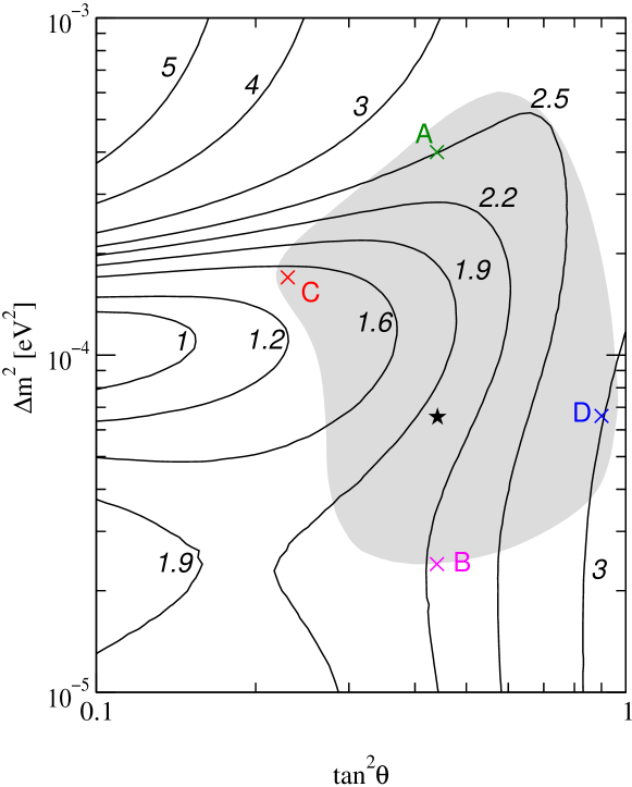
Figure 4: Contours of the 90% C.L. bound on $|\mathbf{\Lambda}|$ in units of $10^{-10}\mu_{B}$ from combined solar and reactor data. The shaded region is the 3$\sigma$ LMA-MSW region from Ref. Maltoni:2002ni , the best fit point is marked with a star. The crosses labeled A, B, C, D are the test points considered in Table 2.

In order to better understand these results we give in Tab. 2 bounds on $|\mathbf{\Lambda}|$ for five characteristic points in the $\tan^{2}\theta-\Delta m^{2}$ plane, including the current best fit point, which is labeled with a star. The other points are marked in Figs. 3 and 4 by crosses and are labeled A, B, C, D, and the corresponding values of the oscillation parameters are given in Tab. 2. Besides the bound on $|\mathbf{\Lambda}|$ we give also bounds on the individual $|\Lambda_{i}|\>(i=1,2,3)$. These bounds are obtained by setting the other two $\Lambda_{i}$ to zero. We show the bounds for the different data samples: solar rates, the shape of the SK spectrum with free overall normalization (SK spect), solar rates combined with the SK spectrum (solar global), reactor data only, solar data combined with reactor data (sol + react).

Notice that, in contrast with the bound on $|\mathbf{\Lambda}|$ which, thanks to Eq. (7), is valid in any basis, the bounds on individual $|\Lambda_{i}|$ do not have a basis-independent meaning. The bounds on $|\Lambda_{i}|$ given in Tab. 2 refer to the mass-eigenstate basis, also used in Ref. Schechter:1981hw .

	solar rates	SK spect	solar global	reactor	sol + react
$\star$	$\tan^{2}\theta=0.44\>,\quad\Delta m^{2}=6.6\times 10^{-5}$ eV2
$|\Lambda_{1}|$	1.8	1.4	1.4	2.0	1.3
$|\Lambda_{2}|$	5.8	4.0	4.0	1.3	1.3
$|\Lambda_{3}|$	1.7	1.4	1.3	1.1	1.0
$|\mathbf{\Lambda}|$	5.8	4.0	4.0	$-$	2.0
A	$\tan^{2}\theta=0.44\>,\quad\Delta m^{2}=4.0\times 10^{-4}$ eV2
$|\Lambda_{1}|$	3.3	2.6	2.6	2.0	2.0
$|\Lambda_{2}|$	3.1	2.3	2.3	1.3	1.4
$|\Lambda_{3}|$	2.2	1.7	1.7	1.1	1.1
$|\mathbf{\Lambda}|$	3.3	2.6	2.6	$-$	2.5
B	$\tan^{2}\theta=0.44\>,\quad\Delta m^{2}=2.4\times 10^{-5}$ eV2
$|\Lambda_{1}|$	01.7	01.5	01.4	2.0	1.4
$|\Lambda_{2}|$	15.5	12.1	11.9	1.3	1.3
$|\Lambda_{3}|$	01.7	01.5	01.4	1.1	1.1
$|\mathbf{\Lambda}|$	15.4	12.0	11.6	$-$	2.3
C	$\tan^{2}\theta=0.23\>,\quad\Delta m^{2}=1.7\times 10^{-4}$ eV2
$|\Lambda_{1}|$	2.3	1.6	1.5	2.6	1.4
$|\Lambda_{2}|$	2.6	1.6	1.5	1.2	1.1
$|\Lambda_{3}|$	1.7	1.1	1.1	1.1	0.9
$|\mathbf{\Lambda}|$	2.6	1.6	1.5	$-$	1.5
D	$\tan^{2}\theta=0.90\>,\quad\Delta m^{2}=6.6\times 10^{-5}$ eV2
$|\Lambda_{1}|$	2.2	1.9	1.9	1.6	1.6
$|\Lambda_{2}|$	8.3	6.3	6.4	1.5	1.6
$|\Lambda_{3}|$	2.2	1.9	1.8	1.1	1.2
$|\mathbf{\Lambda}|$	8.2	6.2	6.2	$-$	3.0

Table 2: 90% C.L. bounds on $|\Lambda_{i}|\>(i=1,2,3)$ and on $|\mathbf{\Lambda}|$ in units of $10^{-10}\mu_{B}$ at fixed points in the $\tan^{2}\theta-\Delta m^{2}$ plane from different data samples. The hyphen indicates that $|\mathbf{\Lambda}|$ cannot be bounded from reactor data alone.

By comparing the first and the second column of Tab. 2 we notice that both solar rates and SK spectrum are important: although the bound from the SK spectrum is slightly stronger, the one which follows from solar rates is in general of the same order. The bound we obtain by combining rates and SK spectrum is displayed in the third column. Concerning the reactor data, clearly these bounds do not depend on $\Delta m^{2}$, and the bound on $|\Lambda_{3}|$ is even completely independent of the neutrino oscillation parameters (see Eq. (15)). As mentioned above, reactor data on their own cannot be used to constrain $|\mathbf{\Lambda}|$.

In the upper parts of the LMA-MSW region, the solar data alone give already a strong bound on $|\mathbf{\Lambda}|$. From the bounds given in Tab. 2 at point A we see that for such high values of $\Delta m^{2}$ all $|\Lambda_{i}|$ are strongly constrained by solar data. This is due to the fact that there the probability $P_{e1}$ relevant in SK is close to the optimal value of 0.5 (see Fig. 1). In this parameter region the combination with reactor data does not improve the bound significantly. This is also true for the region of small $\tan^{2}\theta$ around point C.

The behavior of the bounds for low $\Delta m^{2}$ values can be understood by looking at point B. In this $\Delta m^{2}$ region the probability $P_{e1}$ is very small for the neutrino energies relevant for SK, as seen in Fig. 1. Therefore, solar data give only a very weak constraint on $|\Lambda_{2}|$ as can be seen from Tab. 2, and the bound on $|\mathbf{\Lambda}|$ is dominated by this weak bound on $|\Lambda_{2}|$ (see Eq. (21)) leading to the rather poor bound of $11.6\times 10^{-10}\mu_{B}$ from solar data. In this case the combination with reactor data improves the bound drastically to $2.3\times 10^{-10}\mu_{B}$.

Up to now we have calculated bounds on neutrino TMs for fixed values of the oscillation parameters $\tan^{2}\theta$ and $\Delta m^{2}$ (method I described in Section 3). These results will be especially useful after KamLAND will have determined the oscillation parameters with good accuracy. In the following we change our strategy and minimize the $\chi^{2}$ for each value of $|\mathbf{\Lambda}|$ with respect to $\tan^{2}\theta$ and $\Delta m^{2}$ (method II). This will lead to a bound on $|\mathbf{\Lambda}|$ taking into account the current knowledge concerning the oscillation parameters. To this end we make use of the global solar neutrino data (including earth matter effects) as described in Ref. Maltoni:2002ni in order to obtain the correct $\chi^{2}$ behavior as a function of $\tan^{2}\theta$ and $\Delta m^{2}$. Only in the expression for $\mu^{2}_{\mathrm{LMA}}$ we neglect earth matter effects as described in Section 2, since they are known to be small in the LMA-MSW region earthmatter . Performing this analysis we obtain the following bounds at 90% C.L.:

$$|\mathbf{\Lambda}|<\left\{\begin{array}[]{l@{\quad}l}6.3\times 10^{-10}\mu_{B}&\mbox{(unconstrained, solar data)}\\ 2.0\times 10^{-10}\mu_{B}&\mbox{(unconstrained, solar + reactor data).}\end{array}\right.$$ (32)

Together with Figs. 3 and 4 the bounds given in Eq. (32) constitute an important result of this paper. They show that, assuming the solar LMA-MSW solution, current solar neutrino data can be used to constrain all elements of the Majorana neutrino TM matrix. A combination with data from reactor experiments significantly strengthens the bound on $|\mathbf{\Lambda}|$.

6 Simulation of the Borexino experiment

Here we investigate the sensitivity of the Borexino experiment borexino , Alimonti:2002xc to neutrino TMs. This experiment is mainly sensitive to the solar ⁷Be neutrino flux, which will be measured by elastic neutrino–electron scattering. Therefore, Borexino is similar to SK, the main difference is the mono-energetic line of the ⁷Be neutrinos, with an energy of 0.862 MeV, which is roughly one order of magnitude smaller than the energies of the ⁸B neutrino flux relevant in SK.

6.1 The Borexino $\chi^{2}$-function

To estimate the sensitivity of Borexino we consider the following $\chi^{2}$-function:

$$\chi^{2}_{\mathrm{borexino}}=\sum_{i,j=1}^{N_{\mathrm{bins}}}(N_{i}^{\mathrm{th}}-D_{i})(V^{\mathrm{borex}}_{ij})^{-1}(N_{j}^{\mathrm{th}}-D_{j})\,.$$ (33)

Here $N_{i}^{\mathrm{th}}$ is the theoretical prediction for the number of events in the electron recoil energy bin $i$, and $D_{i}$ is the (hypothetical) observed number of events. Borexino will observe recoil electrons with kinetic energy in the range 0.25 to 0.8 MeV. As a realistic example we adopt $N_{\mathrm{bins}}=8$ bins in electron recoil energy and an energy resolution of 0.058 MeV borexino , Alimonti:2002xc , Berezhiani:2001rt . We have checked that our results are essentially independent of the exact value of the energy resolution.

The theoretical prediction for the number of events in the bin $i$ after $N_{\mathrm{years}}$ years of Borexino data taking is given by

$$N_{i}^{\mathrm{th}}=N_{i}^{\mathrm{weak}}+N_{i}^{\mathrm{em}}(\mu_{\mathrm{LMA}})+N_{i}^{\mathrm{bg}}\,,\quad N_{i}^{x}=365\,N_{\mathrm{years}}\,n_{i}^{x}$$ (34)

with $x=$ th, weak, em, bg, and $n_{i}^{\mathrm{weak,em,bg}}$ is the number of events per day from weak scattering, electromagnetic scattering and the background, respectively. If not stated otherwise we consider a running time of $N_{\mathrm{years}}=3$ years. In order to estimate the sensitivity of Borexino for neutrino TMs we assume that the data are generated by neutrinos without TMs:

$$D_{i}=N_{i}^{\mathrm{weak}}+N_{i}^{\mathrm{bg}}\,.$$ (35)

Hence, we obtain

$$\chi^{2}_{\mathrm{borexino}}=\sum_{i,j=1}^{N_{\mathrm{bins}}}N_{i}^{\mathrm{em}}\,(V^{\mathrm{borex}}_{ij})^{-1}\,N_{j}^{\mathrm{em}}\,.$$ (36)

The minimum of this $\chi^{2}$ occurs for $\mu_{\mathrm{LMA}}=0$ and is always zero. With the $\chi^{2}$ of Eq. (36) we calculate a bound on $|\mathbf{\Lambda}|$ at a given C.L. This bound corresponds to the maximum allowed value of $|\mathbf{\Lambda}|$ which cannot be distinguished from $|\mathbf{\Lambda}|=0$, and is therefore a measure for the obtainable sensitivity to $|\mathbf{\Lambda}|$ at Borexino.

The numbers of events due to the weak and electromagnetic scattering are calculated by

$$n_{i}^{\mathrm{weak}} = \mathcal{N}\sum_{f}\Phi_{f}^{0}\int_{0}^{\infty}dE_{\nu}\,\phi_{f}\left\{P_{ee}^{f}\,[\sigma^{W}_{e}]_{i}+(1-P_{ee}^{f})[\sigma^{W}_{\mu}]_{i}\right\},$$

$$n_{i}^{\mathrm{em}} = \mathcal{N}\sum_{f}\Phi_{f}^{0}\int_{0}^{\infty}dE_{\nu}\,\phi_{f}\,\mu^{2}_{\mathrm{LMA}}\,[\sigma^{\prime}_{\mathrm{em}}]_{i}\,,$$ (37)

respectively. The effective cross sections in the bin $i$ are calculated like in Eqs. (24) and (25), by choosing the lower and upper bounds of the recoil energy interval $T_{1}$ and $T_{2}$ according to the given bin $i$. We sum over the four most important neutrino fluxes ($f$ = Be, pep, N, O) in Borexino (see Ref. Alimonti:2002xc ). For the mono-energetic lines we have $\phi_{\mathrm{Be}}(E_{\nu})=\delta(E_{\nu}-0.862\,\mathrm{MeV})$ and $\phi_{\mathrm{pep}}(E_{\nu})=\delta(E_{\nu}-1.442\,\mathrm{MeV})$, and we use the normalized spectra $\phi_{\mathrm{N}}(E_{\nu})$ and $\phi_{\mathrm{O}}(E_{\nu})$ given in Ref. bahcallpage . The absolute values of the neutrino fluxes $\Phi_{f}^{0}$ from Ref. BP00 are given by $\Phi^{0}_{\mathrm{Be}}=0.429,\,\Phi^{0}_{\mathrm{pep}}=0.014,\,\Phi^{0}_{\mathrm{N}}=0.055,\,\Phi^{0}_{\mathrm{O}}=0.048$ in units of $10^{10}$ cm^-2s^-1. Note that from the two ⁷Be lines the line at 0.38 MeV, which constitutes 10% of the total ⁷Be flux, does not contribute to the signal in Borexino. Therefore the value for $\Phi^{0}_{\mathrm{Be}}$ given above has been obtained by multiplying the value given in Ref. BP00 with 0.9.

flux	7Be	pep	13N	15O	background
events/day	43.3	2.0	4.0	5.5	19

Table 3: Expected number of events per day in Borexino for the kinetic energy of the recoil electrons in the range 0.25 to 0.8 MeV resulting from different components of the SSM solar neutrino flux without neutrino conversion (taken from Table 4 of Ref. Alimonti:2002xc ). Also shown is the expected number of background events per day.

In Table 3 we show the expected number of events per day in Borexino for the kinetic energy of the recoil electrons in the range 0.25 to 0.8 MeV, resulting from different solar neutrino fluxes, for the standard solar model without neutrino oscillations. We do not consider other neutrino fluxes, because they contribute to the signal with less than 0.2 events per day. We fix the normalization constant $\mathcal{N}$ in Eq. (37) in such a way that the number of events per day from the ⁷Be line for $P_{ee}=1$ and $\mu_{\mathrm{LMA}}=0$ is 43.3. Then we can reproduce the number of events arising from the other fluxes as given in Table 3 to good accuracy.

The number of background events $n_{i}^{\mathrm{bg}}$ is obtained in the following way. We read off the shape of the background as a function of the electron energy from Fig. 15 of Ref. Alimonti:2002xc and normalize this function to 19 background events per day in the energy range 0.25 to 0.8 MeV borexino . Then we can calculate $n_{i}^{\mathrm{bg}}$ by integrating over the corresponding energy interval for each bin.

We use the following covariance matrix in Eq. (36):

$$V^{\mathrm{borex}}_{ij}=\delta_{ij}N_{i}^{\mathrm{th}}+\sum_{f_{1},f_{2}}N_{if_{1}}N_{jf_{2}}\sum_{\beta=1}^{12}\alpha_{f_{1}\beta}\alpha_{f_{2}\beta}\left(\Delta\!\ln\!X_{\beta}\right)^{2}+N_{i}^{\mathrm{bg}}N_{j}^{\mathrm{bg}}(\Delta\ln N^{\mathrm{bg}})^{2}\,.$$ (38)

The first term is the statistical uncertainty, taken as the square-root of the predicted number of events. The second term describes the uncertainty in the solar neutrino fluxes. Here $N_{if}$ are the contributions of the individual solar neutrino fluxes to the total event numbers in each bin: $N_{i}^{\mathrm{th}}=\sum_{f}N_{if}+N_{i}^{\mathrm{bg}}$, and the sum is over the four fluxes relevant in Borexino (for definition and values of the quantities $\alpha_{f\beta}$ and $X_{\beta}$ see Ref. fogli ). The last term takes into account a systematic uncertainty in the number of background events. We assume full correlation between the bins and that the relative uncertainty is the same for all bins: $\Delta N_{i}^{\mathrm{bg}}/N_{i}^{\mathrm{bg}}=\Delta\ln N^{\mathrm{bg}}$. We adopt a standard value for our calculations of $\Delta\ln N^{\mathrm{bg}}=10\%$.

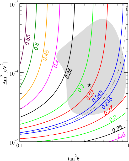
Figure 5: Contours of the 90% C.L. bound on $|\mathbf{\Lambda}|$ after 3 years of Borexino data-taking in units of $10^{-10}\mu_{B}$. The current best fit point is shown by the star, and the shaded region is the allowed LMA-MSW region at 3$\sigma$, from Ref. Maltoni:2002ni . The dotted line corresponds to $P_{e1}=0.5$ for ⁷Be neutrinos.

6.2 Sensitivity on $|\mathbf{\Lambda}|$ of Borexino

Using the statistical method described in Sections 3 and 6.1 we obtain for the current best fit point $\Delta m^{2}=6.6\times 10^{-5}$ eV², $\tan^{2}\theta=0.44$ the upper bound (sensitivity)

$$|\mathbf{\Lambda}|\leq 0.28\times 10^{-10}\mu_{B}\quad\mbox{at}\quad 90\%\>\mbox{C.L.}$$ (39)

after three years of Borexino data taking. This bound is about one order of magnitude stronger than the bound from existing data. We have checked that a combined analysis of Borexino with existing data (solar as well as reactor data) does not improve the bound of Eq. (39). The bound depends on the actual value of the oscillation parameters; in Fig. 5 we show contours of the 90% C.L. bound in the $\tan^{2}\theta-\Delta m^{2}$ plane. The strongest attainable limit is roughly $0.24\times 10^{-10}\mu_{B}$. In agreement with the discussion we gave in connection with Eq. (21) we find that the strongest bound is obtained when $P_{e1}=0.5$, as shown by the dotted line in Fig. 5.

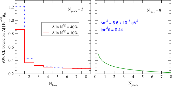
Figure 6: The left panel shows the 90% C.L. bound on $|\mathbf{\Lambda}|$ after 3 years of Borexino data-taking as a function of the number of recoil electron energy bins for two values of the error on the background. The right panel gives the 90% C.L. bound on $|\mathbf{\Lambda}|$ as a function of Borexino running time for $\Delta\ln N^{\mathrm{bg}}=10$%.

We have performed several tests concerning our assumptions for Borexino. Fig. 6 (left panel) shows the dependence of the bound on the number of bins in the recoil electron energy. We can see from this figure that a measurement of the total rate alone ($N_{\mathrm{bins}}=1$) gives a rather weak bound. However a few bins are already enough for a considerable improvement of the bound on $|\mathbf{\Lambda}|$. It is interesting to see that the error on the background is only important for few bins, and becomes completely unimportant for more than 3 or 4 bins, because the main information comes from the spectral shape.

In the right panel in Fig. 6 we show the bound as a function of the Borexino running time. Here we adopt again our nominal value of 8 energy bins. After one year a sensitivity of $0.4\times 10^{-10}\mu_{B}$ can be obtained with Borexino, which is already about one order of magnitude stronger than the current bound. After three years of data-taking only a minor improvement of the bound is possible, mainly due to the uncertainty in the solar neutrino fluxes.

7 Conclusions

In this paper we have presented stringent bounds on electromagnetic Majorana transition moments (TMs). Such TMs—if present—would contribute to the elastic neutrino–electron scattering signal in solar neutrino experiments like Super-Kamiokande or the upcoming Borexino experiment, as well as in reactor neutrino experiments. Motivated by the robust status of the LMA-MSW solution of the solar neutrino problem indicated by recent data, and also by the prospects of its possible confirmation by the KamLAND experiment, we have taken this solution as basis for our investigation. In this context we have clarified which effective magnetic moments are probed in solar and reactor experiments—see Eqs. (12) and (13), respectively. Using most recent global solar neutrino data we have performed a fit in terms of the oscillation parameters and the elements of the complex TM matrix $\lambda$ of three active Majorana neutrinos. Taking into account the antisymmetry of the TM matrix by the parameterization $\lambda_{jk}=\varepsilon_{jkl}\Lambda_{l}$, we have shown that solar neutrino data allow to constrain $|\mathbf{\Lambda}|$, i.e., all elements of the TM matrix are bounded at the same time. We want to stress that the bounds on $|\mathbf{\Lambda}|$ hold in any basis, because $|\mathbf{\Lambda}|$ is an intrinsic neutrino property; in terms of TMs it is given by

$$|\mathbf{\Lambda}|^{2}=|\lambda_{e\mu}|^{2}+|\lambda_{\mu\tau}|^{2}+|\lambda_{\tau e}|^{2}=|\lambda_{12}|^{2}+|\lambda_{23}|^{2}+|\lambda_{31}|^{2}$$ (40)

in the flavour and mass-eigenstate bases, respectively. On the other hand, the bounds on the individual $|\Lambda_{i}|$ ($i=1,2,3$) in Tab. 2 refer only to the mass-eigenstate basis.

A fit to the global solar neutrino data leads to the bound $|\mathbf{\Lambda}|<6.3\times 10^{-10}\mu_{B}$ at 90% C.L. We have also considered the role of reactor neutrino data on neutrino TMs, shown to be complementary to solar neutrino data. A combined fit of reactor and solar data leads to significantly improved bounds: at 90% C.L. we get $|\mathbf{\Lambda}|<2.0\times 10^{-10}\mu_{B}$. In the very near future the KamLAND experiment will crucially test the LMA-MSW solution. If KamLAND confirms the LMA-MSW solution then a precise determination of the parameters $\tan^{2}\theta$ and $\Delta m^{2}$ might be possible. This motivated us to scan the $\tan^{2}\theta-\Delta m^{2}$ plane and to calculate the corresponding bound on $|\mathbf{\Lambda}|$ in each point. These results are shown in Figs. 3 and 4 for solar data and solar + reactor data, respectively.

We have also investigated the potential of the upcoming neutrino–electron scattering solar neutrino experiment Borexino to constrain neutrino TMs. Performing a detailed simulation of the experiment we find that it will improve the bound on $|\mathbf{\Lambda}|$ by about one order of magnitude with respect to present bounds.

Last, but not least, let us mention that alternative solutions to the solar neutrino problem based on non-standard neutrino matter interactions Guzzo:2001mi , which may arise in models of neutrino masses NSImodels , can also be constrained in an analogous way Berezhiani:2001rt . If, as seems likely, the LMA-MSW solution is finally borne out, the improved determination of the oscillation parameters expected, say at KamLAND, will provide an extremely useful stepping stone for probing other features of neutrino physics beyond the Standard Model.

References

- [1] B.T. Cleveland et al., Astrophys. J. 496 (1998) 505.
- [2] J.N. Abdurashitov et al., SAGE Collaboration, astro-ph/0204245.
-
[3]
W. Hampel et al., GALLEX Collaboration,
Phys. Lett. B 447 (1999) 127;
M. Altmann et al., GNO Collaboration, Phys. Lett. B 490 (2000) 16 [hep-ex/0006034]. - [4] S. Fukuda et al., SuperKamiokande Collaboration, Phys. Lett. B 539 (2002) 179 [hep-ex/0205075].
- [5] Q.R. Ahmad et al., SNO Collaboration, Phys. Rev. Lett. 89 (2002) 011301 [nucl-ex/0204008].
- [6] Q.R. Ahmad et al., SNO Collaboration, Phys. Rev. Lett. 89 (2002) 011302 [nucl-ex/0204009].
-
[7]
Atmospheric data were reviewed in the talks by M.
Shiozawa and M. Goodman at the XXth International Conference on
Neutrino Physics and Astrophysics,
http://neutrino2002.ph.tum.de/. - [8] Y. Fukuda et al., Super-Kamiokande Collaboration, Phys. Rev. Lett. 81 (1998) 1562 [hep-ex/9807003].
- [9] M. Maltoni, T. Schwetz, M.A. Tórtola and J.W.F. Valle, hep-ph/0207227.
-
[10]
M.C. Gonzalez-Garcia, P.C. de Holanda, C. Peña-Garay and J.W.F. Valle,
Nucl. Phys. B 573 (2000) 3 [hep-ph/9906469];
J.N. Bahcall, M.C. Gonzalez-Garcia and C. Peña-Garay, hep-ph/0204314;
A. Bandyopadhyay, S. Choubey, S. Goswami and D.P. Roy, Phys. Lett. B 540 (2002) 14 [hep-ph/0204286];
V. Barger, D. Marfatia, K. Whisnant and B.P. Wood, Phys. Lett. B 537 (2002) 179 [hep-ph/0204253];
P.C. de Holanda and A.Yu. Smirnov, hep-ph/0205241;
A. Strumia, C. Cattadori, N. Ferrari and F. Vissani, hep-ph/0205261;
M.V. Garzelli and C. Giunti, Phys. Rev. D 65 (2002) 093005 [hep-ph/0111254];
G.L. Fogli, E. Lisi, A. Marrone, D. Montanino and A. Palazzo, hep-ph/0206162. - [11] G.L. Fogli et al., hep-ph/0208026; M.C. Gonzalez-Garcia, M. Maltoni, C. Peña-Garay and J.W.F. Valle, Phys. Rev. D 63 (2001) 033005 [hep-ph/0009350].
- [12] J. Schechter and J.W.F. Valle, Phys. Rev. D 22 (1980) 2227.
-
[13]
R.N. Mohapatra and P.B. Pal, “Massive Neutrinos in Physics and
Astrophysics” (World Scientific, 1998);
J.W.F. Valle, “Gauge Theories and the Physics of Neutrino Mass”, Prog. Part. Nucl. Phys. 26 (1991) 91 and references therein. - [14] K. Fujikawa and R. Shrock, Phys. Rev. Lett. 45 (1980) 963.
- [15] A.I. Derbin et al., JETP Lett. 57 (1993) 768 [Pisma Zh. Eksp. Teor. Fiz. 57 (1993) 755].
- [16] A.V. Derbin, Phys. Atom. Nucl. 57 (1994) 222 [Yad. Fiz. 57 (1994) 236].
-
[17]
C. Broggini, MUNU Collaboration,
Nucl. Phys. B (Proc. Suppl.) 100 (2001) 267;
J. Vuilleumier, Talk at Neutrino 2002, Munich,http://neutrino2002.ph.tum.de/. - [18] L.B. Auerbach et al., LSND Collaboration, Phys. Rev. D 63 (2001) 112001.
- [19] R. Schwienhorst et al., DONUT Collaboration, Phys. Lett. B 513 (2001) 23.
- [20] K. Hagiwara et al., Particle Data Group, Phys. Rev. D 66 (2002) 010001.
- [21] G.G. Raffelt, Phys. Rept. 320 (1999) 319.
- [22] B.S. Neganov et al., hep-ex/0105083.
- [23] J. Schechter and J.W.F. Valle, Phys. Rev. D 24 (1981) 1883 [Erratum-ibid. D 25 (1982) 283].
-
[24]
E.K. Akhmedov,
Phys. Lett. B 213 (1988) 64;
C.S. Lim and W.J. Marciano, Phys. Rev. D 37 (1988) 1368. -
[25]
O.G. Miranda, C. Peña-Garay, T.I. Rashba, V.B. Semikoz and J.W.F. Valle,
Phys. Lett. B 521 (2001) 299 [hep-ph/0108145];
Nucl. Phys. B 595 (2001) 360 [hep-ph/0005259];
J. Barranco, O.G. Miranda, T.I. Rashba, V.B. Semikoz and J.W.F. Valle, hep-ph/0207326. -
[26]
S.A. Dazeley, KamLAND Collaboration,
hep-ex/0205041;
A. Piepke, KamLAND Collaboration, Nucl. Phys. B (Proc. Suppl.) 91 (2001) 99;
KamLAND web-pagehttp://kamland.lbl.gov/KamLAND. - [27] J.F. Beacom and P. Vogel, Phys. Rev. Lett. 83 (1999) 5222 [hep-ph/9907383].
- [28] A.S. Joshipura and S. Mohanty, Phys. Rev. D 66 (2002) 012003 [hep-ph/0204305].
-
[29]
E. Meroni, Borexino Collaboration,
Nucl. Phys. B (Proc. Suppl.) 100 (2001) 42;
G. Ranucci et al., Borexino Collaboration, Nucl. Phys. B (Proc. Suppl.) 91 (2001) 58;
Borexino web-pagehttp://almime.mi.infn.it/. - [30] G. Alimonti et al., Borexino Collaboration, Astropart. Phys. 16 (2002) 205 [hep-ex/0012030].
- [31] M. Maltoni, T. Schwetz, M.A. Tórtola and J.W.F. Valle, hep-ph/0207157.
-
[32]
D.Y. Bardin, S.M. Bilenky and B. Pontecorvo,
Phys. Lett. B 32 (1970) 68;
A.V. Kyuldjiev, Nucl. Phys. B 243 (1984) 387. - [33] W. Grimus and T. Schwetz, Nucl. Phys. B 587 (2000) 45 [hep-ph/0006028].
- [34] A.S. Dighe, Q.Y. Liu and A.Yu. Smirnov, hep-ph/9903329.
-
[35]
G.L. Fogli, E. Lisi, D. Montanino and A. Palazzo,
Phys. Rev. D 62 (2000) 113003
[hep-ph/0008012];
M.C. Gonzalez-Garcia, C. Peña-Garay and A.Yu. Smirnov, Phys. Rev. D 63 (2001) 113004 [hep-ph/0012313];
A. de Gouvea, A. Friedland and H. Murayama, JHEP 0103 (2001) 009 [hep-ph/9910286]. -
[36]
M. Apollonio et al., CHOOZ Collaboration,
Phys. Lett. B 466 (1999) 415;
F. Boehm et al., Palo Verde Collaboration, Phys. Rev. D 64 (2001) 112001 [hep-ex/0107009]. - [37] J.N. Bahcall, M.H. Pinsonneault and S. Basu, Astrophys. J. 555 (2001) 990.
-
[38]
J.N. Bahcall’s web-page
http://www.sns.ias.edu/~jnb/. - [39] J.N. Bahcall, M. Kamionkowski and A. Sirlin, Phys. Rev. D 51 (1995) 6146 [astro-ph/9502003].
-
[40]
Y. Fukuda et al., Super-Kamiokande Collaboration,
Phys. Rev. Lett. 82 (1999) 2430 [hep-ex/9812011].
For a parameterization see, e.g.,
J.N. Bahcall, P.I. Krastev and E. Lisi, Phys. Rev. C 55 (1997) 494 [nucl-ex/9610010];
B. Faid et al., Phys. Rev. D 55 (1997) 1353 [hep-ph/9608311];
F.L. Villante, G. Fiorentini and E. Lisi, Phys. Rev. D 59 (1999) 013006 [hep-ph/9807360]. - [41] G.L. Fogli, E. Lisi, D. Montanino and A. Palazzo, Phys. Rev. D 62 (2000) 013002.
- [42] Z. Berezhiani, R.S. Raghavan and A. Rossi, hep-ph/0111138.
- [43] M. Guzzo, P.C. de Holanda, M. Maltoni, H. Nunokawa, M.A. Tórtola and J.W.F. Valle, Nucl. Phys. B 629 (2002) 479 [hep-ph/0112310] and references therein.
-
[44]
R.N. Mohapatra and J.W.F. Valle, Phys. Rev. D 34 (1986) 1642;
L.J. Hall, V.A. Kostelecký and S. Raby, Nucl. Phys. B 267 (1986) 415.