SUSY breaking mediation mechanisms and $(g-2)_{\mu}$, $B\rightarrow X_{s}\gamma$,  $B\rightarrow X_{s}l^{+}l^{-}$ and $B_{s}\rightarrow\mu^{+}\mu^{-}$

Abstract

We show that there are qualitative differences in correlations among $(g-2)_{\mu}$, $B\rightarrow X_{s}\gamma$, $B\rightarrow X_{s}l^{+}l^{-}$ and $B_{s}\rightarrow\mu^{+}\mu^{-}$ in various SUSY breaking mediation mechanisms: minimal supergravity (mSUGRA), gauge mediation (GMSB), anomaly mediation (AMSB), gaugino mediation ($\tilde{g}$MSB), weakly and strongly interacting string theories, and $D$ brane models. After imposing the direct search limits on the Higgs boson and SUSY particle search limits and $B\rightarrow X_{s}\gamma$ branching ratio, we find all the scenarios can accommodate the $a_{\mu}\equiv(g-2)_{\mu}/2$ in the range of (a few tens)$\times 10^{-10}$, and predict that the branching ratio for $B\rightarrow X_{s}l^{+}l^{-}$ can differ from the standard model (SM) prediction by $\pm 20\%$ but no more. On the other hand, the $B_{s}\rightarrow\mu^{+}\mu^{-}$ is sensitive to the SUSY breaking mediation mechanisms through the pseudoscalar and stop masses ($m_{A}$ and $m_{\tilde{t}_{1}}$), and the stop mixing angle. In the GMSB with a small messenger number, the AMSB, the $\tilde{g}$MSB and the noscale scenarios, one finds that $B(B_{s}\rightarrow\mu^{+}\mu^{-})\lesssim 2\times 10^{-8}$, which is below the search limit at the Tevatron Run II. Only the mSUGRA or string inspired models can generate a large branching ratio for this decay.

I Introduction

The minimal supersymmetric standard model (MSSM) is widely regarded as the leading candidate for the physics beyond the standard model (SM) nilles . Its detailed phenomenology both in the flavor preserving and flavor changing sectors are heavily dependent on soft SUSY breaking lagrangians which contain 105 new parameters (including CP violating phases) compared to the SM. This indicates that our understanding of SUSY breaking and mechanisms mediating SUSY breaking to our world is not complete yet, although many suggestions have been put forward over the past 20 years or so. There are various models on soft terms in the literatures : gravity mediation (SUGRA) mSUGRA , gauge mediation (GMSB)  gauge , anomaly mediated SUSY breaking (AMSB) amsb , and no–scale noscale or gaugino mediation ($\tilde{g}$MSB) ginomsb , etc., to name a few representative mechanisms. Each mechanism predicts sparticle spectra and the trilinear couplings which could be qualitatively different from one to another scenarios. It is most important to determine the soft parameters from various different experiments, and compare the resulting soft SUSY breaking parameters with those predicted in the aformentioned SUSY breaking mediation mechanisms. This process will provide invaluable informations on the origin of SUSY breaking, which may be intrinsically rooted in very high energy regimes such as intermediate, GUT or Planck scales.

Direct productions of SUSY particles and measuring their properties are the best ways for this purpose. However, the importance of indirect effects of SUSY particles through quantum loop corrections cannot be underestimated at all for the following reasons. First of all, the experimental errors in many low energy processes are now already (or will be in the near future) at the level of probing the loop effects from SUSY particles : the muon $(g-2)$, $B\rightarrow X_{s}\gamma$, $B\rightarrow X_{s}l^{+}l^{-}$, $B_{s}\rightarrow\mu^{+}\mu^{-}$, etc., to name a few. On the other hand, theoretical uncertainties, which are mainly from our poor understanding of (non)perturbative QCD effects, are becoming larger than the experimental errors, and it is very important to reduce these theoretical uncertainties before one can say a definite thing about a possible presence of some new physics beyond the SM from these low energy observables. Assuming this is achieved at some satisfactory level, we can study the indirect effect of SUSY particles within various SUSY breaking mediation mechanisms. Secondly, the high energy processes available at colliders are usually insensitive to the flavor structures of soft SUSY breaking parameters. On the other hand, the low energy favor changing neutral current (FCNC) processes such as $B-\overline{B}$ and $K-\overline{K}$ mixings as well as $B$ and $K$ decays can be very sensitive to such nontrivial flavor structures in soft terms. Therefore, once some observables are dominated by short distance physics and thus can be reliably calculable in renormalization group (RG) improved perturbations theory, these may give us some hints for possible existence of new physics beyond the SM with nontrivial flavor structures.

In this work, we consider the following low energy processes, the muon $(g-2)_{\mu}$, $B\rightarrow X_{s}\gamma$, $B\rightarrow X_{s}l^{+}l^{-}$ and $B_{s}\rightarrow\mu^{+}\mu^{-}$ for various SUSY breaking mediation mechanisms : SUGRA, GMSB, AMSB, $\tilde{g}$MSB and certain classes of string theories where dilaton/T/M moduli are the mediators. It turns out there are qualitative differences among various correlations for different SUSY breaking mediation mechanisms, especially depending on the messenger scale. This qualitative difference may help us to distinguish various SUSY breaking mediation mechanisms from low energy processes, in addition to the informations provided by high energy collider experiments.

Suppose that the positive $\mu$ is preferred by the BNL data on $a_{\mu}$. Then, the Wilson coefficient $C_{7,\gamma}$ for the process $B\rightarrow X_{s}\gamma$ in SUSY models (except for AMSB) turns out to have the same sign as in the SM case. And the sign of $C_{7}$ can be (partly) observed in $B\rightarrow X_{s}l^{+}l^{-}$ (or some exclusive channels) and FB asymmetry therein. Therefore the correlations between the $B\rightarrow X_{s}\gamma$ and $B\rightarrow X_{s}l^{+}l^{-}$ will depend on the sign $(\mu)$ and the SUSY breaking mediation mechanisms. Since the ongoing $B$ factory experiments began to observe $B\rightarrow Kl^{+}l^{-}$, it would be timely to include the decay $B\rightarrow X_{s}l^{+}l^{-}$ into our analysis. Furthermore, if $\tan\beta$ should be moderately large in order to fit the BNL data on $(g-2)_{\mu}$, the SUSY QCD corrections to $h-b-\bar{b}$ can change by a significant amount hall ; hbb , thereby affecting $B_{s}\rightarrow\mu^{+}\mu^{-}$ by a (potentially) significant amount dedes . This decay may be observable at the Tevatron Run II down to the level of $2\times 10^{-8}$. Therefore this decay can cover parameter space (large $\tan\beta$ region) which is not accessible by direct search for SUSY particles at the Tevatron Run II. All these correlations will depend on the sign of the $\mu$ parameter, $\tan\beta$ and the detailed spectra of SUSY particles which are determined by soft SUSY breaking parameters. Still, we could foresee that there may be qualitative differences in some correlations among these observables through different chargino, stop, pseudoscalar masses $(m_{\chi^{+}},m_{\tilde{t_{1}}},m_{A})$ depending on $\tan\beta$, $\mu$, $M_{3}$ and the messenger scale $M_{\rm mess}$. The partial results in the GMSB and AMSB were reported in Ref. bks . Similar study on the Higgs boson physics has been recently reported in Ref. heynemeyer . Also the muon $g-2$ in various SUSY breaking mediation mechanisms were considered in Ref. kchoi , including the collier phenomenology tata (see refs. kane for the recent study). In our work, we include $B\rightarrow X_{s}l^{+}l^{-}$ and $B_{s}\rightarrow\mu^{+}\mu^{-}$, and find a qualitative difference among various SUSY breaking mediation mechanisms in the $B_{s}\rightarrow\mu^{+}\mu^{-}$ mode.

This work is organized as follows. In Sec. II, we discuss $a_{\mu}^{\rm SUSY}$, $B\rightarrow X_{s}\gamma$, $B\rightarrow X_{s}l^{+}l^{-}$ and $B_{s}\rightarrow\mu^{+}\mu^{-}$ in the SM and MSSM in brief. In Sec. III, we review various SUSY breaking mediation mechanisms, and present numerical analsyses for various low energy processes. Then the results are summarized in Sec. IV.

II Relevant processes and analysis procedures

II.1 Muon anomalous magnetic moment : $a_{\mu}$

Let us define the $l_{i}\rightarrow l_{j}\gamma$ form factor $F_{ji}(0)$ as follows:

$${\cal L}_{\rm eff}(l_{i}\rightarrow l_{j}\gamma)=e\frac{m_{l_{i}}}{2}~{}\overline{l}_{j}\sigma^{\mu\nu}F_{\mu\nu}\left[F_{ji}^{L}(0)P_{L}+F_{ji}^{R}(0)P_{R}\right]l_{i}.$$ (1)

Then, the muon $(g-2)$ or $a_{\mu}$ is related with $F_{22}^{L(R)}$ by

$$a_{\mu}={1\over 2}~{}(g_{\mu}-2)=m_{\mu}^{2}\left[F^{L}_{22}(0)+F^{R}_{22}(0)\right],$$ (2)

The SM contribution to $a_{\mu}$ had been calculated up to $O(\alpha^{5})$ in QED, up to two loops in the electroweak gauge interactions. Hadronic contributions are composed of vacuum polarization and light-light scattering parts, and are the source of the largest theoretical uncertainties. The BNL data is $116\;591\;597(67)\times 10^{-11}$. Comparing the BNL data of the year 2001 $a_{\mu}=116\;591\;597(67)\times 10^{-11}$ with the most recently updated SM prediction, one finds that g-2

$$\Delta a_{\mu}\equiv a_{\mu}^{\rm SUSY}\equiv a_{\mu}^{\rm exp}-a_{\mu}^{\rm SM}=(26\pm 16)\times 10^{-10}.$$ (3)

We assume that this small deviation can be explained by SUSY effects.

The SUSY contributions to $a_{\mu}$ come from the chargino-sneutrino and the neutralino-smuon loop, the former of which is dominant in most parameter space. Schematically, the result can be written as martin

$$a_{\mu}^{\rm SUSY}={\tan\beta\over 48\pi}{m_{\mu}^{2}\over M_{\rm SUSY}^{2}}(5\alpha_{2}+\alpha_{1})=14\times 10^{-10}~{}\tan\beta~{}\left({100~{}{\rm GeV}\over M_{\rm SUSY}}\right)$$ (4)

in the limit where all the superparticles have the same mass $M_{\rm SUSY}$. In particular, the positive $\mu$ parameter implies the positive $a_{\mu}^{\rm SUSY}$ in our convention. The current value for the deviation between the BNL data bnl and the most recently updated SM prediction g-2 , $(26\pm 16)\times 10^{-10}$, can not be taken as a strong indication for new physics beyond the SM. Therefore, we do not use $a_{\mu}$ as a constraint but give predictions for it. If the data is updated with smaller statistical and systematic errors and theoretical uncertainties, $a_{\mu}^{\rm SUSY}$ could provide a useful constraint on SUSY parameter space. If there is no strong indication for new physics from the upcoming BNL data on the muon $(g-2)_{\mu}$, it would rule out light SUSY spectra and/or large $\tan\beta$ region. Also effective SUSY models will be in more comfortable situations than before (see however Refs. ko ).

II.2 $B\rightarrow X_{s}\gamma$ and $B\rightarrow X_{s}l^{+}l^{-}$

It is well known that the $B\rightarrow X_{s}\gamma$ branching ratio puts a severe constraint on new physics, especially SUSY models from early days of SUSY phenomenology. The relevant effective Hamiltonian for this decay is

$$H_{\rm eff}(b\rightarrow s\gamma)=-{4G_{F}\lambda_{t}\over\sqrt{2}}\left[C_{7L}O_{7L}+C_{7R}O_{7R}\right],$$ (5)

where $\lambda_{t}=V_{ts}^{*}V_{tb}(=-A\lambda^{2})$ in the Wolfenstein parametrization wolfenstein ) and

$$O_{7L}={e\over(4\pi)^{2}}~{}m_{b}\bar{s}_{L}^{\alpha}\sigma^{\mu\nu}b_{R}^{\alpha}~{}F_{\mu\nu}.$$ (6)

The operator $O_{7R}$ is obtained from $O_{7L}$ by the exchange $(L\leftrightarrow R)$. Similarly one can expect a new physics contribution to $b\rightarrow sg$ :

$$H_{\rm eff}(b\rightarrow sg)=-{4G_{F}\lambda_{t}\over\sqrt{2}}\left[C_{8L}O_{8L}+C_{8R}O_{8R}\right],$$ (7)

where

$$O_{8L}={g_{s}\over(4\pi)^{2}}~{}m_{b}\bar{s}_{L}^{\alpha}\sigma^{\mu\nu}T^{a}_{\alpha\beta}b_{R}^{\beta}~{}G^{a}_{\mu\nu},$$ (8)

and $O_{8R}$ is obtained from $O_{8L}$ by the exchange $(L\leftrightarrow R)$. These two processes $b\rightarrow s\gamma$ and $b\rightarrow sg$ are unique in the sense that they are described in terms of only two independent operators $O_{7(8)L}$ and $O_{7(8)R}$ whatever new physics there are. This fact makes it easy to study these decays in a model independent manner kn98 . The SM predictions for the $C_{7,8}$ at the $M_{W}$ scale are (in the limit $m_{s}=0$)

$$C_{7L}^{\rm SM}(M_{W}) \approx -0.22,$$

$$C_{7R}^{\rm SM}(M_{W}) = 0,$$

$$C_{8L}^{\rm SM}(M_{W}) \approx -0.12,$$

$$C_{8R}^{\rm SM}(M_{W}) = 0.$$ (9)

Note that $C_{7(8)R}^{\rm SM}$ in the SM is suppressed compared to $C_{7(8)L}^{\rm SM}$ by $m_{s}/m_{b}$, because $W$ boson couples only to the left-handed fermions. Such terms proportional to $m_{s}$ will be neglected in our work by setting $m_{s}=0$ whenever they appear.

The magnetic dipole coefficient $C_{7,\gamma}$ for this decay receives contributions from SM, charged Higgs and SUSY particles in the loop. The charged Higgs contributions always add up to the SM contributions, thereby increasing the rate. On the other hand, the chargino-stop loop can interfere with the SM and the charged Higgs contributions either in a constructive or destructive manner depending on the sign of $\mu$, and could provide an important constraint on the SUSY parameter space. The gluino loop contribution to $B\rightarrow X_{s}\gamma$ is always negligible in the models we consider in this work. The most recent data belle1 ; cleo

$$Br(B\rightarrow X_{s}\gamma)_{\rm exp}=(3.21\pm 0.43_{(stat)}\pm 0.27_{(sys)-0.10(th)}^{~{}~{}~{}~{}~{}~{}~{}+0.18})\times 10^{-4},$$

is in good agreement with the SM prediction kagan ; bsgamma :

$$Br(B\rightarrow X_{s}\gamma)^{\rm SM}_{E_{\gamma}>1.6GeV}=(3.57\pm 0.30)\times 10^{-4}.$$

Thus, there is very little room for new physics contributions, unless SUSY contributions interfere destructively with the SM contributions.

The inclusive decay $B\rightarrow X_{s}l^{+}l^{-}$ has been also considered extensively in the context of two Higgs doublet modelbsll2hd , mSUGRA bsllsugra model, GMSB  bsllgmsb and SUSY models with minimal flavor violations  bsllmfv as well as in the SM bsllsm . Here the local $\bar{s}b\bar{l}l$ operators are also important as well as the nonlocal photon exchange diagram due to $C_{7,\gamma}$. In the presence of new physics contributions to $b\rightarrow s\gamma$, there should be also generic new physics contributions to $b\rightarrow sl^{+}l^{-}$ through electromagnetic penguin diagrams. This effect will modify the Wilson coefficient $C_{9}$ of the dim-6 local operator $O_{9}$ :

$$H_{\rm eff}(b\rightarrow sll)\supset H_{\rm eff}(b\rightarrow s\gamma)-{4G_{F}\lambda_{t}\over\sqrt{2}}~{}\left[C_{9}O_{9}+C_{10}O_{10}\right]$$

$$-{4G_{F}\lambda_{t}\over\sqrt{2}}~{}\left[C_{S}O_{S}+C_{P}O_{P}+C_{S}^{{}^{\prime}}O_{S}^{{}^{\prime}}+C_{P}^{{}^{\prime}}O_{P}^{{}^{\prime}}\right],$$ (10)

where the operators $O_{9}$, $O_{10}$, $O_{S}$ and $O_{P}$ are defined by

$$O_{9}={e^{2}\over(4\pi)^{2}}\left(\overline{s}_{L}\gamma_{\mu}b_{L}\right)~{}(\overline{l}\gamma^{\mu}l), O_{10}={e^{2}\over(4\pi)^{2}}\left(\overline{s}_{L}\gamma_{\mu}b_{L}\right)~{}(\overline{l}\gamma^{\mu}\gamma_{5}l),$$

$$O_{S}={e^{2}\over(4\pi)^{2}}~{}(\overline{s}_{L}b_{R})~{}(\overline{l}l), O_{P}={e^{2}\over(4\pi)^{2}}~{}(\overline{s}_{L}b_{R})~{}(\overline{l}\gamma_{5}l).$$ (11)

The primed operators are obtained by the exchange $L\leftrightarrow R$ on the quark bilinear operators.

In the SM, the Wilson coefficients $C_{9,10}$’s are given by

$$C_{9}^{\rm SM}(M_{W})\approx 2.01,~{}~{}~{}C_{10}^{\rm SM}(M_{W})\approx 4.55.$$ (12)

In fact, the latter is important when the dilepton invariant mass $m_{ll}$ is low because of the photon propagator effect $1/m_{ll}^{2}$ in the amplitude. The SM predictions in NLO for $l=e$ and $\mu$ are bsllsm

$$B(B\rightarrow X_{s}e^{+}e^{-}) = (6.3^{+1.0}_{-0.9})\times 10^{-6},$$

$$B(B\rightarrow X_{s}\mu^{+}\mu^{-}) = (5.7\pm 0.8)\times 10^{-6},$$ (13)

respectively. Although the inclusive decays are difficult to measure with high precision, the ongoing B factory experiments began to be sensitive to exclusive decay modes although the experimental errors are large bsllexp :

$$B(B\rightarrow Kl^{+}l^{-}) < 0.6\times 10^{-6}~{}~{}~{}[0.47-0.75]$$

$$B(B\rightarrow K\mu^{+}\mu^{-}) = (0.99^{+0.40+0.13}_{-0.32-0.14})\times 10^{-6}~{}~{}~{}[0.47-0.75]$$

$$B(B\rightarrow K^{*}e^{+}e^{-}) < 5.0\times 10^{-6}~{}~{}~{}[1.4-3.0]$$

$$B(B\rightarrow K^{*}\mu^{+}\mu^{-}) = 3.6\times 10^{-6}~{}~{}~{}[0.9-2.4]$$

The SM predictions shown in the brackets (in units of $10^{-6}$) suffer from large theoretical uncertainties because the form factors are poorly known bsllth . In view of these data, it is quite timely to consider this class of processes in various SUSY breaking mediation mechanisms.

This implies that in the $C_{7}$ coefficient for $B\rightarrow X_{s}\gamma$ process, the chargino contribution interfere destructively with the SM and the charged Higgs contributions. However, this does not imply that $C_{7}$ necessarily has the opposite sign to the $C_{7}^{\rm SM}$. For sufficiently large $\tan\beta$ (namely, for large $a_{\mu}^{SUSY}$), it is possible to have $C_{7}^{\rm MSSM}\approx-C_{7}^{\rm SM}$. Then the branching ratio for $B\rightarrow X_{s}l^{+}l^{-}$ will be substantially larger than the SM case. In other words, if the deviation in $a_{\mu}$ is larger than the current value, it is very likely that the branching ratio for $B\rightarrow X_{s}l^{+}l^{-}$ should be significantly enhanced compared to the SM predictions.

In order to avoid the hadronic uncertainties related with exclusive $B$ decays and the long distance contributions from charmonia and charmed meson intermediate states, we consider inclusive $B\rightarrow X_{s}l^{+}l^{-}$ below the $J/\psi$ resonance. Defining

$$R_{\mu\mu}\equiv{B(B\rightarrow X_{s}\mu^{+}\mu^{-})_{\rm MSSM}\over B(B\rightarrow X_{s}\mu^{+}\mu^{-})_{\rm SM}}$$ (14)

in the region with

$$2m_{\mu}\leq m_{\mu\mu}\leq(m_{J/\psi}-100~{}{\rm MeV}).$$

In this region, the nonlocal contributions from the virtual photon exchange involving $O_{7\gamma}$ is more important than the local four fermion operators $O_{9}$ and $O_{10}$. Therefore the ratio $R_{\mu\mu}$ is strongly correlated with the branching ratio of $B\rightarrow X_{s}\gamma$ and the sign of $C_{7\gamma}(m_{b})$. The forward backward asymmetry of dilepton energy distributions in the rest frame of the parent $B$ meson can be a sensitive probe of new physics. However we postpone studying this observable for the future project, and will not consider in the present work.

II.3 Hall–Rattazzi–Sarid Effect

Another important effect in the large $\tan\beta$ limit is the nonholomorphic SUSY QCD corrections to the $h-b-\bar{b}$ couplings, the so-called Hall – Rattazzi – Sarid effect hall . Also for large $A_{t}$ and $y_{t}$ couplings, the stop – chargino loop could be quite important. One can summarize these effects as the following relation between the bottom quark mass and the bottom Yukawa coupling $y_{b}$ hbb :

$$m_{b}=y_{b}{\sqrt{2}M_{W}\cos\beta\over g}~{}(1+\Delta_{b})$$ (15)

where

$$\Delta_{b} \simeq {2\alpha_{s}\over 3\pi}~{}M_{\tilde{g}}\mu\tan\beta I(M_{\tilde{b}_{1}},M_{\tilde{b}_{2}},M_{\tilde{g}})$$ (16)

$$+ {\alpha_{t}\over 4\pi}~{}A_{t}\mu\tan\beta I(M_{\tilde{t}_{1}},M_{\tilde{t}_{2}},\mu)$$

and the loop integral $I(a,b,c)$ is given by

$$I(a,b,c) = \left[a^{2}b^{2}\log(a^{2}/b^{2})+b^{2}c^{2}\log(b^{2}/c^{2})+c^{2}a^{2}\log(c^{2}/a^{2})\right]/$$

$$\left[(a^{2}-b^{2})(b^{2}-c^{2})(a^{2}-c^{2})\right]$$

Therefore in the large $\tan\beta$ limit, the SUSY loop correction $\Delta_{b}$ can be large as well with either sign, depending on the sign of the $\mu$ parameter and the gluino mass parameter $M_{\tilde{g}}$. Note that the muon $(g-2)$ picks up $\mu>0$, whereas the $B\rightarrow X_{s}\gamma$ prefers a positive $\mu M_{\tilde{g}}$.

II.4 $B_{s}\rightarrow\mu^{+}\mu^{-}$

The effective Hamiltonian for $B_{s}\rightarrow l^{+}l^{-}$ is already given in Eqs. (10) (11), and the branching ratio for this decay is given by arnowitt

$$B(B_{s}\rightarrow\mu^{+}\mu^{-}) = {G_{F}^{2}\alpha^{2}\tau_{B}M_{B}^{5}\over 64\pi^{3}}~{}f_{B_{s}}^{2}~{}\left|\lambda_{t}\right|^{2}\sqrt{1-{4m_{\mu}^{2}\over M_{B_{s}}^{2}}}$$ (17)

$$\left[\left(1-{4m_{\mu}^{2}\over M_{B_{s}}^{2}}\right)~{}\left|{(C_{S}-C_{S}^{{}^{\prime}})\over(m_{b}+m_{s})}\right|^{2}+\left|{(C_{P}-C_{P}^{{}^{\prime}})\over(m_{b}+m_{s})}+2{m_{\mu}\over M_{B_{s}}^{2}}(C_{10}-C_{10}^{{}^{\prime}})\right|^{2}\right].$$

The branching ratio for the decay $B_{s}\rightarrow\mu^{+}\mu^{-}$ is very small in the SM : $(3.7\pm 1.2)\times 10^{-9}$ dedes . The current upper limit from CDF during Tevatron Run I is set to $<2.6\times 10^{-6}$ at 95 % C.L. bsmmexp At Tevatron Run II, CDF aims at achieving a single event sensitivity down to $10^{-8}$ for an integrated luminosity of 2 fb^-1. In SUSY models, both $B\rightarrow X_{s}l^{+}l^{-}$ huang ; Choudhury:1998ze and $B_{d}\rightarrow\mu^{+}\mu^{-}$ babu ; Huang:2000sm can be significantly enhanced in the large $\tan\beta$ limit, due to the neutral Higgs boson exchange, and similarly for the analogous process $B_{s}\rightarrow\mu^{+}\mu^{-}$. The SUSY effects are encoded in the Wilson coefficients $C$’s. For large $\tan\beta$, one has, for example,

$$C_{S}\simeq\left({\tan^{3}\beta\over 4\sin^{2}\theta_{W}}\right)~{}\left({m_{b}m_{\mu}m_{t}\mu\over M_{W}^{2}M_{A}^{2}}\right)~{}{\sin 2\theta_{\tilde{t}}\over 2}~{}f(m_{\tilde{t_{1}}}^{2},m_{\tilde{t_{2}}}^{2},\mu^{2}).$$

Here, $C_{P}=-C_{S}$, $C_{S}^{{}^{\prime}}=(m_{s}/m_{b})C_{S}$ and $C_{P}^{{}^{\prime}}=-(m_{s}/m_{b})C_{P}$, and the loop function $f(x,y,z)$ can be found in Refs. dedes ; arnowitt ; babu ; Chankowski ; Urban ; cgnw ; isidori . (See also Refs. cpv for the discussions for CP violations therein.) Note that the branching ratio for this decay is proportional to $\tan^{6}\beta$, and thus can be enhanced by a significant amount for large $\tan\beta$, light pseudoscalar boson ($m_{A}$), light stop ($m_{\tilde{t}_{1}}$) and the large $\tilde{t}_{L}-\tilde{t}_{R}$ mixing angle $\theta_{\tilde{t}}$. The Hall – Rattazzi – Sarid effect can further modify the result in either direction depending on the sign$(\mu)$. For $\mu>0$, the enhancement becomes less pronounced due to the Hall-Rattazzi-Sarid effect.

II.5 Constraints

When we scan over SUSY parameter space, we impose the direct search limits on Higgs and SUSY particles (except for the GMSB scenario) heynemeyer :

$$m_{\tilde{e},\tilde{\mu},\tilde{\tau},\tilde{\nu}} > 95,~{}~{}85,~{}~{}71,~{}~{}43~{}{\rm GeV},$$

$$m_{\tilde{t},\tilde{b},\tilde{g}} > 95,~{}~{}85,~{}~{}190~{}{\rm GeV},$$

$$m_{\chi^{+}}^{\rm mSUGRA} > 103~{}{\rm GeV~{}for}~{}m_{\tilde{\nu}}>300~{}{\rm GeV},$$

$$m_{\chi^{+}}^{\rm mSUGRA} > 83.6~{}{\rm GeV~{}for}~{}m_{\tilde{\nu}}<300~{}{\rm GeV},$$

$$m_{\chi^{+}}^{\rm AMSB} > 45~{}{\rm GeV},$$

$$m_{\chi^{0}}^{\rm mSUGRA} > 36~{}{\rm GeV},$$

$$m_{\chi^{0}}^{\rm AMSB} > 45~{}{\rm GeV}.$$ (18)

For the GMSB, the LSP is always very light gravitinos, and we impose

$$m_{\rm NLSP}^{\rm GMSB}>100~{}{\rm GeV},$$ (19)

which is stronger than other experimental bounds on SUSY particle masses. It turns out that the stau mass bound is quite strong in a certain region of parameter space.

In order to be as model independent as possible, we do not assume that the LSP is color and charge neutral (except for the GMSB scenario where the gravitino is the LSP), nor do we impose the color-charge breaking minima or the unbounded from below constraints munoz ; casas ; abel , since these constraints can be evaded in nonstandard cosmology.

Also we impose the $B\rightarrow X_{s}\gamma$ branching ratio as a constraint. Then, using the aforementioned constraints, we find that the sign of $C_{7,\gamma}$ for $B\rightarrow X_{s}\gamma$ cannot flip relative to the SM case, and the branching ratio for $B\rightarrow X_{s}l^{+}l^{-}$ remains close to the SM prediction. (Note that the previous study in the context of mSUGRA suggested that two branches would be possible for $Br(B\rightarrow X_{s}\gamma)$ for large $\tan\beta$, because of both sign of $C_{7,\gamma}$ were allowed.) Therefore there is no chance to observe $B\rightarrow X_{s}l^{+}l^{-}$ at the level of $70\%-80\%$ enhanced over to the SM. For the muon $(g-2)$, we do not use it as a constraint but give predictions for it, since the current value for the deviation between the BNL data and the most updated SM prediction, $(26\pm 16)\times 10^{-10}$, can not be taken as a serious indication for new physics beyond the SM.

II.6 Procedures

First of all, we assume the radiative electroweak symmetry breaking (REWSB) to trade $\mu$ and $B\mu$ with $M_{Z}$ and $\tan\beta$ using the following relations:

$$\mu^{2} = {m_{H_{d}}^{2}-m_{H_{u}}^{2}\tan^{2}\beta\over\tan^{2}\beta-1}-{1\over 2}M_{Z}^{2},$$

$$B\mu = (m_{H_{d}}^{2}+m_{H_{u}}^{2}+2\mu^{2})\sin 2\beta,$$ (20)

where $m_{H_{d}}^{2}$ and $m_{H_{u}}^{2}$ are loop corrected running masses for two Higgses (which are soft SUSY breaking). The sign of $\mu$ is fixed to be positive but we do not assume anything about $\tan\beta$. There is no problem to accommodate the $a_{\mu}\sim+O(10)\times 10^{-10}$ in SUSY models we consider in this work, except for the AMSB scenario. The decay $B\rightarrow X_{s}\gamma$ will be in good shape for $\mu>0$, since the chargino loop contribution can cancel the charged Higgs contributions for the positive $\mu$. The data will constrain the absolute value of $C_{7\gamma}(m_{b})$. Then, for a small $\tan\beta$, the predicted branching ratio for $B\rightarrow X_{s}l^{+}l^{-}$ is essentially the same as the SM prediction. On the other hand, for large $\tan\beta$, one can have either signs of $C_{7\gamma}$ so that the branching ratio for $B\rightarrow X_{s}l^{+}l^{-}$ can take two values for a given $B\rightarrow X_{s}\gamma$ branching ratio. However, in the SUSY breaking mediation scenarios we consider, it turns out that the current lower bound on the Higgs boson is too severe that the parameter space in which the branching ratio for $B\rightarrow X_{s}l^{+}l^{-}$ becomes large with $C_{7\gamma}\approx-C_{7\gamma}^{\rm SM}$ is essentially excluded. Therefore there is little hope to observe a large deviation in Br ($B\rightarrow X_{s}\gamma$). This is true for the minimal SUGRA scenario, in particular, and this observation is newly made in the present work for the first time to our best knowledge. On the other hand, the decay $B_{s}\rightarrow\mu^{+}\mu^{-}$ depends on the stop mass and the stop mixing angle, which are sensitive to the SUSY breaking mediation mechanisms and the messenger scale. So we anticipate there are qualitative differences in the predictions for $B(B_{s}\rightarrow\mu^{+}\mu^{-})$. In order to have a light stop and large $\tilde{t}_{L}-\tilde{t}_{R}$ mixing, it is crucial to have a large messenger scale and a lighter squark mass parameter at the messenger scale. Then RG running will produce the stop mass and the $A_{t}$ parameter which determine the stop mixing. This phenomenon will be most clearly seen in the GMSB scenario with different messenger scale and different number of the messenger fields (see Sec. III B).

III SUSY Breaking Mediation Mechanisms

In this section, we review several SUSY breaking mediation mechanisms : minimal SUGRA, gauge mediated SUSY breaking, anomaly mediated SUSY breaking, gaugino mediated SUSY breaking ($\tilde{g}$MSB) (which includes the no–scale supergravity scenario), weakly interacting superstring models with dilaton and moduli mediations, heterotic $M$ theory and $D-$brane models. When we give expressions for the soft SUSY braking parameters, we assume that all the parameters are real in order to avoid SUSY CP problem. It would be straightforward to relax this assumption with substantial complications in the numerical analysis, which we do not aim to do in this work. Thus there is no new source of CP violations beyond the KM phase in the CKM mixing matrix. Also scalar fermion masses are unversal in many cases, so that the SUSY flavor problem is mitigated significantly.

III.1 Minimal Supergravity (mSUGRA)

Supergravity theories, which may be a low energy effective field theory of more fundamental theories such as superstring or $M$ theories, are completely specified by three objects:

• Kähler potential $K(\Phi,\Phi^{*},V,V^{\dagger})$: a real scalar function of chiral and vector superfields $\Phi_{i}$ and $V$ in the visible sector, respectively

• Gauge kinetic functions $f_{ab}(\Phi)$: a holomorphic function of chiral superfields $\Phi$, where $a,b$ are gauge group indices

• Superpotential $W(\Phi)$: a holomorphic function of chiral superfield

The holomorphic functions $f_{ab}(\Phi)$ and $W(\Phi)$ are protected from the radiative corrections by nonrenormalization theorem, whereas the Kähler potential will be renormalized in general. All the couplings may depend on the hidden sector fields or moduli (we denote these fields collectively by $\Sigma$), although we suppressed this dependence. From these three objects, one can derive the soft terms such as the sfermion masses, trilinear couplings, gaugino masses.

If one assumes a simple form for the Kähler potential, $K=\sum_{i}\Phi_{i}^{*}\Phi_{i}+\sum_{j}X_{j}^{*}X_{j}$ with $X_{j}$ hidden sector fields, the soft parameters satisfy universal sfermion masses $m_{0}$. If the Yukawa couplings in the superpotential $W(\Phi)$ is assumed to be constant independent of the hidden fields or modulis ($\Sigma$), we get universal trilinear coupling $A_{0}$ with exact proportionality. Assuming that the gauge kinetic function is independent of the gauge group, one has the universal gaugino mass $M_{1/2}$. Although these specific assumptions are ad hoc out of question, it leads to a simple universality in the scalar mass and trilinear couplings at the GUT scale so that SUSY flavor problem can be signifiantly mitigated. Also a restricted set of mSUGRA models can be motivated in the string inspired SUGRA models where a dilaton plays a dominant role in SUSY breaking mediation (see Sec. II E). One can also relax the condition for the gaugino unification at GUT scale. In this case, low energy phenomenology can be richer, and there could be qualitative changes in our results. But we keep the gaugino unification assumption in this work in order to reduce the number of parameters, relegating the study of nonuniversal gaugino mass scenarios for the future publication. Under these assumtions, the mSUGRA model is specified by the following five parameters :

$$m_{0},~{}~{}M_{1/2},~{}~{}A_{0},~{}~{}\tan\beta,~{}~{}{\rm sign}(\mu).$$ (21)

We scan these parameters over the following ranges :

$$50~{}{\rm GeV} \leq M_{1/2}\leq 1~{}{\rm TeV},$$

$$1.5 \leq \tan\beta\leq 60,$$ (22)

with $A_{0}=0$, $m_{0}=300$ GeV and $\mu>0$. For a negative $\mu$, we have $a_{\mu}^{\rm SUSY}<0$ and also the $B\rightarrow X_{s}\gamma$ constraint becomes much more severe since the chargino-stop loop interferes constructively with the SM and the charged Higgs loop contributions. Earlier phenomenological analysis of mSUGRA scenarios can be found on the muon $(g-2)_{\mu}$, $B\rightarrow X_{s}\gamma$ and $B\rightarrow X_{s}l^{+}l^{-}$, bsllsugra , for example.

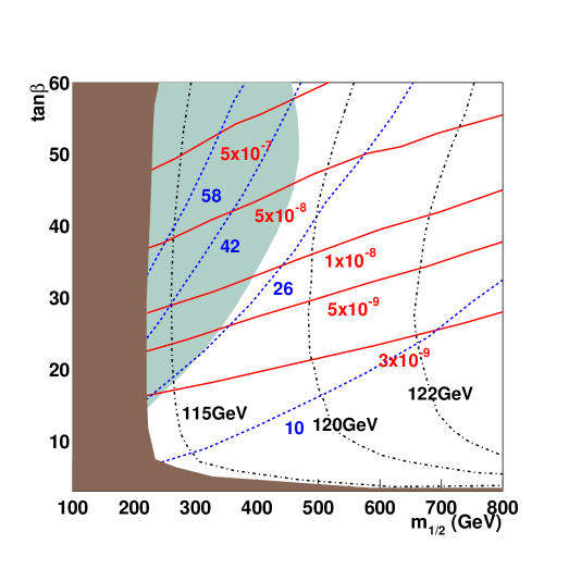
Figure 1: The contour plots for $a_{\mu}^{\rm SUSY}$ in unit of $10^{-10}$ (in the short dashed curves) and the Br ($B_{s}\rightarrow\mu^{+}\mu^{-}$) (in the solid curves) in $(m_{1/2},\tan\beta)$ plane in the minimal SUGRA model for $m_{0}=300$ GeV and $A_{0}=0$. The brown (dark) region is excluded by the Higgs and SUSY particle mass bounds, and the green (light gray) region is excluded by $B\rightarrow X_{s}\gamma$ branching ratio.

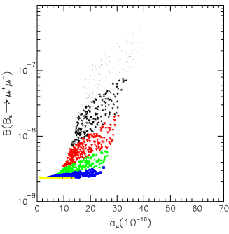
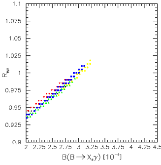
Figure 2: The correlations between (a) the muon $a_{\mu}^{\rm SUSY}$ and $B(B_{s}\rightarrow\mu^{+}\mu^{-})$, and (b) $Br(B\rightarrow X_{s}\gamma)$ and $R_{\mu\mu}$ in the mSUGRA model with $A_{0}=0$ and $m_{0}=300$ GeV. The regions Different colors represent different ranges of $\tan\beta$: $3\leq\tan\beta\leq 10$ (yellow), $10\leq\tan\beta\leq 20$ (blue), $20\leq\tan\beta\leq 30$ (green), $30\leq\tan\beta\leq 40$ (red), $40\leq\tan\beta\leq 50$ (black star) and $50\leq\tan\beta$ (black dots).

In Fig. 1, we show the constant contour plots for $a_{\mu}^{\rm SUSY}$ in unit of $10^{-10}$ (in the short dashed curves) and the Br ($B_{s}\rightarrow\mu^{+}\mu^{-}$) (in the solid curves) in the $(M_{1/2},\tan\beta)$ plane for $m_{0}=300$ GeV and $A_{0}=0$. The left dark region is excluded by direct search limits on SUSY particles and Higgs boson masses, and the light gray region is excluded by the lower bound on the $B\rightarrow X_{s}\gamma$. The dot–dashed contours corresponds to $m_{h}=115,120,122$ GeV’s for the future reference. The result for $B_{s}\rightarrow\mu^{+}\mu^{-}$ is essentially the same as the Fig. 2 of Dedes et al. dedes , except that we did not assume that the LSP should be color/charge neutral but did impose $B\rightarrow X_{s}\gamma$ at 95 % CL.

In Fig. 2 (a), we show the correlation between the muon $a_{\mu}^{\rm SUSY}$ and $B(B_{s}\rightarrow\mu^{+}\mu^{-})$. For convenience, we represent different $a_{\mu}^{\rm SUSY}$’s with different shapes (also different colors). The regions $a_{\mu}^{\rm SUSY}<10\times 10^{-10}$, $10\times 10^{-10}<a_{\mu}^{\rm SUSY}<26\times 10^{-10}$, $26\times 10^{-10}<a_{\mu}^{\rm SUSY}<42\times 10^{-10}$, $42\times 10^{-10}<a_{\mu}^{\rm SUSY}<58\times 10^{-10}$, and $a_{\mu}^{\rm SUSY}>58\times 10^{-10}$ are represented by the stars (black), the inverted triangles (red), the triangles (green), the squares (blue) and the circles (yellow). The $B_{s}\rightarrow\mu^{+}\mu^{-}$ branching ratio can be enhanced up to $2\times 10^{-7}$ ($\sim 6\times 10^{-7}$) for large $\tan\beta$, if we impose (do not impose) $B\rightarrow X_{s}\gamma$ constraint. The current upper limit from CDF : $2.6\times 10^{-6}$ (95 % C.L.), and large $\tan\beta$ region of the mSUGRA model will be within the reach of Tevatron Run II by searching the $B_{s}\rightarrow\mu^{+}\mu^{-}$ decay mode down to the level of $\sim 2\times 10^{-8}$. In the region where $B_{s}\rightarrow\mu^{+}\mu^{-}$ branching ratio is larger than $10^{-7}$, the $a_{\mu}^{\rm SUSY}$ is around $(20-30)\times 10^{-10}$, which is much larger than the aimed experimental uncertainties. On the other hand, this enhancement effect diminishes quickly as $\tan\beta$ (and $a_{\mu}^{\rm SUSY}$) becomes smaller. If the new BNL data on $a_{\mu}^{\rm SUSY}$ turns out small ($\lesssim 15\times 10^{-10}$), the $B_{s}\rightarrow\mu^{+}\mu^{-}$ branching ratio cannot be larger than $10^{-8}$ and there would be no chance to observe this decay at the Tevatron Run II.

The correlation between the Br ($B\rightarrow X_{s}\gamma$) and $R_{\mu\mu}$ is an interesting quantity as well, since it can be useful to determine the sign of the $C_{7\gamma}$ coefficient. In Fig. 2 (b), we show this correlation in the mSUGRA model. The $R_{\mu\mu}$ can be enhanced up to 13 % compared to the SM prediction for large $\tan\beta$, but no more. In particular the sign of $C_{7\gamma}$ in the mSUGRA model is the same as the SM case, although there is some destructive interference between the SM and charged Higgs contributions and the chargino-stop contribution. In the previous comprehensive analyses by KEK group  bsllsugra , it was noted that there could be two branch for this correlation imposing the direct search limits available as of 1998. It was due to the possibility to have $C_{7,\gamma}\approx-C_{7,\gamma}^{\rm SUSY}$ for light chargino and stops for the positive $\mu(>0)$. Now this is no longer true when the direct search limits are updated. The lower limits on Higgs boson and other SUSY particles rule out the parameter space in which $C_{7,\gamma}\approx-C_{7,\gamma}^{\rm SUSY}$. Also note that the large $\tan\beta$ region allows a smaller branching ratio for $B\rightarrow X_{s}\gamma$, because the chargino-stop contributions grows as $\tan\beta$ becomes large and it interfere with the SM and the charged Higgs contributions in a destructive manner. Considering experimental and theoretical uncertainties, it would not be possible to use $R_{\mu\mu}$ to indirectly probe the mSUGRA effects. This is also true for other scenarios we consider in this work.

III.2 Gauge Mediated SUSY Breaking (GMSB)

In the gauge mediated SUSY breaking (GMSB), SUSY breaking in the hidden sector is mediated to the observable sector through SM gauge interactions of $N_{\rm mess}$ messenger superfields $\Psi_{i},\Psi_{i}^{c}$, which lie in the vectorlike representation of the SM gauge group. The messenger fields couple to a gauge singlet superfield $X$ through

$$W=\lambda_{i}X\Psi_{i}\Psi_{i}^{c}.$$

The vev of $X$ (both in the scalar and the $F$ components) will induce SUSY breaking in the messenger sector, which in turn induce the following set of SUSY breaking soft parameters in the MSSM sector at the messenger scale $M_{\rm mess}$ :

$$M_{a}(M_{\rm mess}) = N_{\rm mess}\Lambda~{}g\left({\Lambda\over M^{2}_{\rm mess}}\right)~{}{\alpha_{a}\over 4\pi},$$

$$m_{ij}^{2}(M_{\rm mess}) = 2N_{\rm mess}\Lambda^{2}~{}f\left({\Lambda\over M^{2}_{\rm mess}}\right)~{}\sum_{a}\left({\alpha_{a}\over 4\pi}\right)^{2}~{}C_{a}$$

$$A_{ijk}(M_{\rm mess}) = 0.$$ (23)

Here $\alpha_{a}$ (with $a=3,2,1$) are the SM gauge couplings of $SU(3)_{c}\times SU(2)_{L}\times U(1)_{Y}$, $C_{a}^{i}$’s are the quadratic Casimir invariant of the MSSM matter fields, and $f(x)$ and $g(x)$ are loop functions whose explicit form can be found in Ref. gauge . In the limit $\Lambda<<M^{2}_{\rm messenger}$, these loop functions $g(x)$ and $f(x)$ are well approximated to one: $f(x)\approx g(x)\approx 1$ for $x<<1$. We have normalized the $U(1)_{Y}$ charge to a GUT group such as $SU(5)$. Also we have ignored the nonvanishing results for $A_{ijk}$ which arise from two-loop diagrams, since they are suppressed by loop factors. Therefore the free parameters in GMSB are

$$M_{\rm mess},~{}~{}N_{\rm mess},~{}~{}\Lambda,~{}~{}\tan\beta,~{}~{}{\rm sign}(\mu),$$

where $N$ is the number of messenger superfields, $M$ is the messenger scale, and the $\Lambda$ is SUSY breaking scale :

$$\Lambda\approx\langle F_{X}\rangle/\langle X\rangle.$$

In practice, we trade $\Lambda$ for the bino mass parameter $M_{1}$, and we scan these parameters over the following ranges :

$$10^{4}~{}{\rm GeV} \leq \Lambda\leq 2\times 10^{5}~{}{\rm GeV},$$

$$N_{\rm mess} = 1,~{}~{}5$$

$$M_{\rm mess} = 10^{6}{\rm GeV},~{}~{}{\rm and}~{}~{}10^{15}~{}{\rm GeV}.$$ (24)

Earlier phenomenological analysis of GMSB scenarios can be found on the muon $(g-2)_{\mu}$ gmsb:amu , $B\rightarrow X_{s}\gamma$ and $B\rightarrow X_{s}l^{+}l^{-}$, bsllgmsb . The discussion of $B_{s}\rightarrow\mu^{+}\mu^{-}$ in the GMSB scenarios is given in this work for the first time.

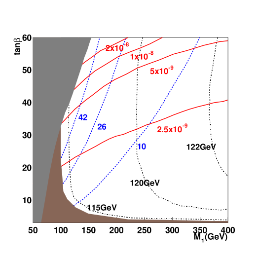
Figure 3: The contour plots for $a_{\mu}^{\rm SUSY}$ in unit of $10^{-10}$ (in the short dashed curves) and the Br ($B_{s}\rightarrow\mu^{+}\mu^{-}$) (in the solid curves) in the $(M_{1},\tan\beta)$ plane in the GMSB model with $N_{\rm mess}=1$ and $M_{\rm mess}=10^{6}$ GeV. The light gray region is excluded by the light stau mass bound, and the brown (dark) region is excluded by the lower bounds on the masses of Higgs bosons.

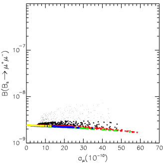
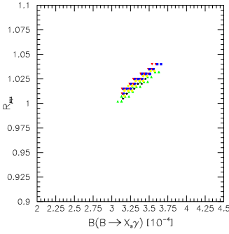
Figure 4: The correlations of the $Br(B\rightarrow X_{s}\gamma)$ with (a) $R_{\mu\mu}$, and (b) $a_{\mu}^{\rm SUSY}$ in the GMSB scenario with $N_{\rm mess}=1$ and $M_{\rm mess}=10^{6}$ GeV. The legends are the same as Fig. 2.

In Fig. 3, we show the contour plots for the $a_{\mu}^{\rm SUSY}$ and $B(B_{s}\rightarrow\mu^{+}\mu^{-})$ in the $(M_{1},\tan\beta)$ plane for $N_{\rm mess}=1$ and $M_{\rm mess}=10^{6}$ GeV. The left dark region is excluded by direct search limit on Higgs boson mass, and the gray region is excluded by the lower bound on the NLSP mass, which is quite significant. For a low $M_{\rm mess}$ scale, the RG runs only for a short distance and its effects are not very large. The resulting $A_{t}$ parameter at the electroweak scale is very small, leading to negligible $\tilde{t}_{L}-\tilde{t}_{R}$ mixing. Also the stop mass is relatively large in this case. Therefore both the chargino-stop and the charged Higgs - top contributions to $B\rightarrow X_{s}\gamma$ are not that important, and there is no strong constraint from $B\rightarrow X_{s}\gamma$. By the same token, the branching ratio for $B_{s}\rightarrow\mu^{+}\mu^{-}$ is always smaller than $10^{-8}$, and this becomes unobservable at the Tevatron Run II. Therefore if the $a_{\mu}^{\rm SUSY}$ turns out to be positive and the decay $B_{s}\rightarrow\mu^{+}\mu^{-}$ is observed at the Tevatron Run II, the GMSB scenarios with low messenger scales would be excluded. $R_{\mu\mu}$ tends to decrease down to 0.9, but this is no significant deviation from the SM prediction, and it would not be possible to observe indirect SUSY signals from $B\rightarrow X_{s}\mu^{+}\mu^{-}$ (See Figs. 4 (a) and (b)).

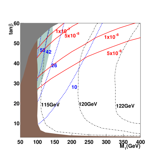
Figure 5: The contour plots for $a_{\mu}^{\rm SUSY}$ in unit of $10^{-10}$ (in the short dashed curves) and the Br ($B_{s}\rightarrow\mu^{+}\mu^{-}$) (in the solid curves) in the $(M_{1},\tan\beta)$ plane for the GMSB model with $N_{\rm mess}=1$ and $M_{\rm mess}=10^{15}$ GeV. The gray region is excluded by the NLSP mass bound, and the green region is excluded by $B\rightarrow X_{s}\gamma$ branching ratio.

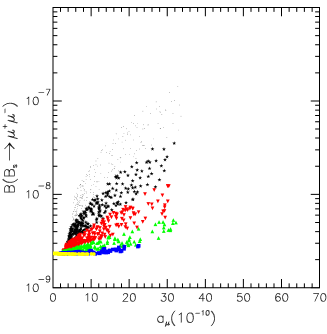
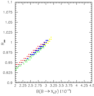
Figure 6: The correlations of the $Br(B\rightarrow X_{s}\gamma)$ with (a) $R_{\mu\mu}$, and (b) $a_{\mu}^{\rm SUSY}$ in the GMSB scenario with $N_{\rm mess}=1$ and $M_{\rm mess}=10^{15}$ GeV. The legends are the same as Fig. 2.

If the messenger scale becomes as high as the GUT scale, the RG effects become important. The $A_{t}$ parameter at the electroweak scale becomes larger, leading to large $\tilde{t}_{L}-\tilde{t}_{R}$ mixing. Therefore, the chargino-stop contribution begins to compensate the SM and charged Higgs - top contributions to $B\rightarrow X_{s}\gamma$. The overall features look alike the mSUGRA or the dilaton dominated case (see Figs. 5 and 6). Still the resulting branching ratio for $B_{s}\rightarrow\mu^{+}\mu^{-}$ is fairly small, and can be as large as $2\times 10^{-8}$ for very large $\tan\beta\sim 60$, and much smaller for $\tan\beta\lesssim 50$. So one can safely assert that the GMSB with $N_{\rm mess}=1$ is excluded if the decay $B_{s}\rightarrow\mu^{+}\mu^{-}$ is discovered at the Tevatron Run II. (This is also true for the case of the minimal AMSB scenario and noscale scenario as discussed in the following subsection.)

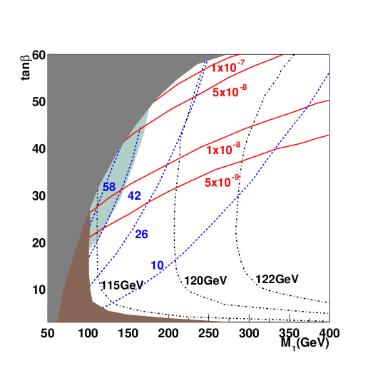
Figure 7: The contour plots for $a_{\mu}^{\rm SUSY}$ in unit of $10^{-10}$ (in the short dashed curves) and the Br ($B_{s}\rightarrow\mu^{+}\mu^{-}$) (in the solid curves) in the $(M_{1},\tan\beta)$ plane for the GMSB model with $N_{\rm mess}=5$ and $M_{\rm mess}=10^{15}$ GeV. The gray region is excluded by the NLSP mass bound, and the green region is excluded by $B\rightarrow X_{s}\gamma$ branching ratio.

As the number of the messenger fields $N_{\rm mess}$ increases from 1 to 5, scalar fermions get lighter compared to the lower $N_{\rm mess}$ case for unified gaugino masses. Therefore, the chargino-stop contributions to $B\rightarrow X_{s}\gamma$ and $B_{s}\rightarrow\mu^{+}\mu^{-}$ become more important than the lower $N_{\rm mess}$ case. Still $B\rightarrow X_{s}\gamma$ is not constraining, but the $B_{s}\rightarrow\mu^{+}\mu^{-}$ branching ratio can be enhanced significantly, like in the mSUGRA model (see Fig. 7). The muon $a_{\mu}^{\rm SUSY}$ can be up to $48\times 10^{-10}$, and the $B_{s}\rightarrow\mu^{+}\mu^{-}$ branching ratio can be enhanced up to $2\times 10^{-7}$. The messenger scale dependence is similar to the previous case, and will not be repeated here.

In summary, the lighter stop mass in the GMSB scenario with $N_{\rm mess}=1$ is generically heavy, although it gets lighter if the messenger scale becomes higher and the RG effects become more important. Still the resulting $B_{s}\rightarrow\mu^{+}\mu^{-}$ branching ratio is smaller than $2\times 10^{-8}$, and only for very large $\tan\beta\approx 60$ this upper limit can be achieved. In most parameter space, it is much smaller, and there would no chance to observe it at Tevatron Run II. On the other hand, if the number of messenger fields and the messenger scale increases, the pseudoscalar and the stop get lighter and the $A_{t}$ parameter gets larger leading to the large stop mixing. Thus the branching ratio for $B_{s}\rightarrow\mu^{+}\mu^{-}$ can be enhanced within the reach of the Tevatron Run II.

III.3 Anomaly Mediated SUSY Breaking (AMSB)

In the AMSB scenario, it is assumed that the hidden sector SUSY breaking is mediated to our world only through the auxiliary component of the supergravity multiplet. This is possible if the Kähler potential has the so-called sequestered form :

$$K=-3\log\left[\xi(\Phi,\Phi^{\dagger})+\zeta(z,z^{\dagger})\right],$$ (25)

where $\Phi$ and $z$ are the observable and the hidden fields, respectively. In this case, the compensator field $X$ will take a VEV of the form :

$$\langle X\rangle=1+F_{X}\theta^{2}$$ (26)

Here $F_{X}$ is an auxiliary field in the gravity supermultiplet, whose VEV is given by (assuming the vanishing cosmological constant)

$$F_{X}={1\over M_{*}^{2}}~{}\left(W+{1\over 3}{\partial K\over\partial z}F_{z}\right),$$ (27)

where $M_{*}\approx 2.4\times 10^{18}$ GeV is the reduced Planck scale.

The soft terms can be extracted by expanding the supergravity lagrangian in the background with nonvanishing $F_{\Phi}$. The results are the following :

$$M_{a} = -{b_{a}\alpha_{a}\over 4\pi}~{}M_{\rm aux},$$

$$m_{ij}^{2} = \left(-{\dot{\gamma}\over 4}~{}M_{\rm aux}^{2}+m_{0}^{2}\right)~{}\delta_{ij},$$

$$A_{ijk} = {1\over 2}~{}(\gamma_{i}+\gamma_{j}+\gamma_{k})M_{\rm aux}.$$ (28)

Here $b_{a}=(3,-1,-33/5)$ (with $a=3,2,1$) are the one-loop beta function coefficients for the SM gauge group $SU(3)_{c}\times SU(2)_{L}\times U(1)_{Y}$, $\gamma_{i}\equiv-d\ln Z_{i}/d\ln\mu$ is the anomalous dimension of the field $\Phi_{i}$, and the dot acting on $\gamma_{i}$ denotes the differentiation with respect to $\ln\mu$. We have simply added $m_{0}^{2}$ to the scalar fermion mass parameters of the original AMSB model in order to avoid the tachyon problem in the slepton sector, and will assume that the above set of equations make initial conditions at the GUT scale for the RG equations. Note that in the pure AMSB case ($m_{0}^{2}=0$) the soft terms are scale invariant so that they are valid for arbitrary scale and are completely fixed by a single overall scale $M_{\rm aux}$ and the gauge couplings at low energy. However this nicety is lost when we add $m_{0}^{2}$ to the scalar fermion masses. Thus, the minimal AMSB model is specified by the following four parameters :

$$\tan\beta,~{}~{}{\rm sign}(\mu),~{}~{}m_{0},~{}~{}M_{\rm aux}.$$

We scan these parameters over the following ranges :

$$20~{}{\rm TeV} \leq m_{\rm aux}\leq 100~{}{\rm TeV},$$

$$0 \leq m_{0}\leq 2~{}{\rm TeV},$$

$$1.5 \leq \tan\beta\leq 60,$$ (29)

Earlier phenomenological analysis of the minimal AMSB scenarios can be found on the muon $(g-2)_{\mu}$ and $B\rightarrow X_{s}\gamma$  amsb:amu ; kchoi ; martin , and on $B_{s}\rightarrow\mu^{+}\mu^{-}$ bks . The discussion on $B\rightarrow X_{s}l^{+}l^{-}$ in the AMSB scenarios is given in this work for the first time.

In the brane world scenarios which became popular during recent years, the Kähler potential takes a sequestered form Eq. (25) in a natural way. The resulting scalar fermion masses take the above form (flavor independent) so that the SUSY flavor problem is solved in the AMSB model. However, Anisimov et al. recently argued that this form is not generic in the brane world SUSY breaking scenario dine . The bulk supergravity effects generate tree level scalar fermion masses which are generically flavor dependent. Only a certain special class of models have zero tree level scalar masses and thus become genuine AMSB models (see, for example, harnik ). In this work, we consider this class of models where the above expressions for the soft terms make good descriptions. This general remark is also true of the gaugino mediation (and no-scale supergravity) scenario(s) to be discussed in the subsequent subsection.

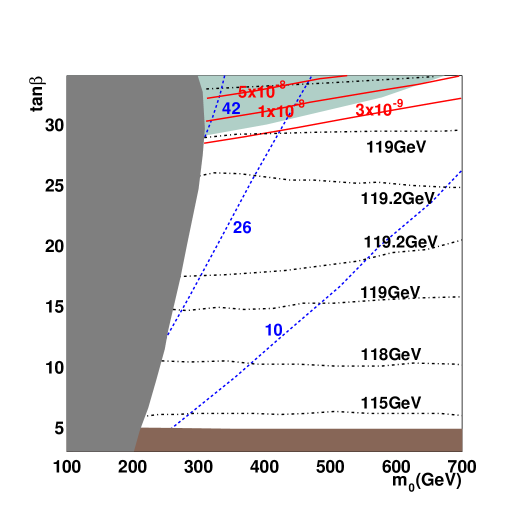
Figure 8: The contour plots for $a_{\mu}^{\rm SUSY}$ in unit of $10^{-10}$ (in the short dashed curves) and the Br ($B_{s}\rightarrow\mu^{+}\mu^{-}$) (in the solid curves) in the $(m_{0},\tan\beta)$ plane for the minimal AMSB scenarios with $M_{\rm aux}=50$ TeV and $\mu>0$. The brown (dark), the gray and the green regions are excluded by the Higgs mass bound, the SUSY particle search, and $B\rightarrow X_{s}\gamma$ branching ratio, respectively.

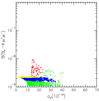
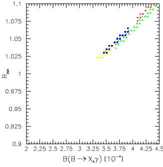
Figure 9: The correlations of (a) $Br(B_{s}\rightarrow\mu^{+}\mu^{-})$ with $a_{\mu}$, and (b) $Br(B\rightarrow X_{s}\gamma)$ with $R_{\mu\mu}$ in the minimal AMSB scenario for $M_{\rm aux}=50$ TeV. The legends are the same as Fig. 2.

In Fig. 8, we show the contour plots for the $a_{\mu}^{\rm SUSY}$ and $B(B_{s}\rightarrow\mu^{+}\mu^{-})$ in the $(m_{0},\tan\beta)$ plane for $M_{\rm aux}=50$ TeV. The low $\tan\beta$ region is excluded by the lower limit on the neutral Higgs boson (the dark region), and the small $m_{0}$ region is strongly constrained by the stau mass bound (the gray region). In the case of the AMSB scenario with $\mu>0$, the $B\rightarrow X_{s}\gamma$ constraint is even stronger compared to other scenarios, since the chargino-stop contribution is additive to the SM and the charged Higgs contribution because of $\mu M_{3}<0$ in the AMSB scenario . This is represented by the green (light gray) region in Fig. 8. Almost all the parameter space with large $\tan\beta>30$ is excluded by the upper limit on $B\rightarrow X_{s}\gamma$. Also stop mass becomes much heavier in the AMSB scenario compared to the mSUGRA or noscale scenarios. This makes the decay $B_{s}\rightarrow\mu^{+}\mu^{-}$ unobservable at the Tevatron Run II, since its branching ratio cannot be larger than $4\times 10^{-9}$. Note that the reason for the small $B_{s}\rightarrow\mu^{+}\mu^{-}$ branching ratio in the GMSB with low $N_{\rm mess}$ or in the AMSB scenarios is heavy stop masses so that chargino-stop loop contribution is suppressed. In the no scale scenario, on the other hand, lighter stop can be much lighter but this region of parameter space is excluded by Higgs and SUSY particle mass bounds. Therefore, if the $a_{\mu}^{\rm SUSY}$ turns out to be positive and the decay $B_{s}\rightarrow\mu^{+}\mu^{-}$ is observed at the Tevatron Run II, the minimal AMSB scenario would be excluded. Also there is no significant deviation in $R_{\mu\mu}$ from 1, and it would not be possible to observe indirect SUSY signals from $B\rightarrow X_{s}\mu^{+}\mu^{-}$ (See Figs. 9 (a) and (b)).

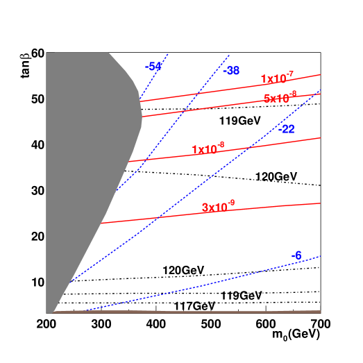
Figure 10: The contour plots for $a_{\mu}^{\rm SUSY}$ in unit of $10^{-10}$ (in the short dashed curves) and the Br ($B_{s}\rightarrow\mu^{+}\mu^{-}$) (in the solid curves) in the $(m_{0},\tan\beta)$ plane for the minimal AMSB scenarios with $M_{\rm aux}=50$ TeV and $\mu<0$.

In the AMSB model, the $B\rightarrow X_{s}\gamma$ is less constraining for the negative $\mu<0$. In this case, the $a_{\mu}$ is also negative, which is marginally consistent with the current data on the muon $(g-2)$. For large $\tan\beta$, the $B_{s}\rightarrow\mu^{+}\mu^{-}$ can be enhanced up to $6\times 10^{-7}$, for which the $a_{\mu}^{\rm SUSY}$ should be also large with the negative sign. All these features can be observed in Fig. 10, where we show the contour plots for the $a_{\mu}^{\rm SUSY}$ and $B(B_{s}\rightarrow\mu^{+}\mu^{-})$ in the $(m_{0},\tan\beta)$ plane for $M_{\rm aux}=50$ TeV and the negative $\mu<0$.

III.4 No-scale and Gaugino Mediated SUSY Breaking

If we assume the following nonminimal Kähler potential and the gauge kinetic function in supergravity models,

$$K=-3\ln(T+T^{*}-\Phi_{i}^{*}\Phi_{i}),~{}~{}~{}f_{ab}=\delta_{ab}T/4\pi~{}(a=1,2,3),$$ (30)

we get

$$M_{a}=M_{\rm aux},~{}~{}~{}m_{ij}^{2}=0,~{}~{}~{}A_{ijk}=0,$$ (31)

at the messenger scale close to the GUT scale. Therefore, only gauginos become massive, and other soft parameters are simply zero including the gravitino masses. Thus the name “no-scale SUGRA” naturally arises noscale . Since the scalar fermion masses and trilinear couplings take the simplest form to be flavor conserving, namely zero, at the messenger scale, SUSY flavor problem is significantly mitigated up to corrections due to the RG effects when we run the above parameters down to the electroweak scale. This no-scale scenario was a popular alternative to the mSUGRA scenario discussed in the Sec. II A. However both scenarios assumed very specific and add hoc forms for the Kähler potential and the gauge kinetic functions, and thus were not justified well from deeper theoretical frameworks.

After the role of branes began to be understood better and included into the particle physics model building, it was realized that the no-scale scenario could be naturally realized in the higher dimensional spacetime. Suppose that the SUSY breaking occurs on a hidden brane, the MSSM matter fields are confined to the visible brane which is distinct from the hidden brane where SUSY is broken, and gauge fields live in the bulk. Then SUSY breaking can be felt by the bulk gauge supermultiplets, thereby generating soft masses for gauginos. Due to the locality in the extra dimension, the soft terms for the MSSM matter fields on the visible brane has to vanish. Only the gaugino can develop nonzero masses at the compactification scale $M_{c}$. The scalar fermions get SUSY breaking masses only through loop effects involving gauginos. This scenario is called the gaugino$(\tilde{g})$ mediation ginomsb . In the gaugino mediated SUSY breaking scenario ($\tilde{g}$MSB), the model parameters are

$$\tan\beta,~{}~{}{\rm sign}(\mu),~{}~{}M_{\rm aux}~{}~{},B=m_{ij}^{2}=A_{ijk}=0$$

at the compactification scale $M_{c}$. If we relax $B=0$ condition, the gaugino mediation model becomes the so-called no-scale supergravity with the corresponding Kähler potential being the same as Eq. (32). Earlier phenomenological analysis of $\tilde{g}$MSB scenarios and noscale scenario can be found on the muon $(g-2)_{\mu}$ and $B\rightarrow X_{s}\gamma$ kchoi ; tata . The discussions of $B\rightarrow X_{s}l^{+}l^{-}$ and $B_{s}\rightarrow\mu^{+}\mu^{-}$ in the no scale scenarios including the $\tilde{g}$MSB scenarios is given in this work for the first time.

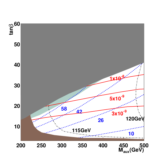
Figure 11: The contour plots for $a_{\mu}^{\rm SUSY}$ in unit of $10^{-10}$ (in the short dashed curves) and the Br ($B_{s}\rightarrow\mu^{+}\mu^{-}$) (in the solid curves) in the $(M_{\rm aux},\tan\beta)$ plane for the noscale scenario. The light gray region is excluded by the light stau mass bound, and the green region is excluded by the lower bound to the $B\rightarrow X_{s}\gamma$ branching ratio.

In Fig. 11, we show the contour plots for the $a_{\mu}^{\rm SUSY}$ and $B(B_{s}\rightarrow\mu^{+}\mu^{-})$ in the $(M_{\rm aux},\tan\beta)$ plane. The black region is excluded by direct search limits on SUSY and Higgs particles, and the green (light gray) denote the region excluded by the $B\rightarrow X_{s}\gamma$ constraint. The dark gray region is excluded by the stau/smuon limit. In the allowed parameter space, the $a_{\mu}^{\rm SUSY}$ can easily become up to $\sim 70\times 10^{-10}$ and one can easily accommodate the BNL data. On the other hand, the branching ratio for $B_{s}\rightarrow\mu^{+}\mu^{-}$ is always smaller than $2\times 10^{-8}$ and becomes unobservable at the Tevatron Run II, as in the AMSB models. This is because the large $\tan\beta$ region, where the branching ratio for $B_{s}\rightarrow\mu^{+}\mu^{-}$ can be much enhanced, is significantly constrained by lighter stau and smuon mass bounds and the lower bound of $B\rightarrow X_{s}\gamma$. Therefore if the $a_{\mu}^{\rm SUSY}$ turns out to be positive and the decay $B_{s}\rightarrow\mu^{+}\mu^{-}$ is observed at the Tevatron Run II, the noscale scenario would be excluded. Also there is an anticorrelation between $R_{\mu\mu}$ and $B(B\rightarrow X_{s}\gamma)$ and varies between 0.95 and 1.14. Thus it would not be possible to observe indirect SUSY signals from $B\rightarrow X_{s}\mu^{+}\mu^{-}$. Noscale SUGRA models with non universal gaugino masses are discussed in Ref. noscale2 .

III.5 Deflected anomaly mediation

The deflected anomaly mediation damsb is a kind of combination of pure anomaly mediation with gauge mediation scenario. If a heavy threshold arises from SUSY breaking effects, integrating out the heavy degree of freedoms would kick the low energy SUSY breaking parameters off the pure AMSB trajectories and solve the tachyonic slepton problem. The model contains a light singlet $X$ which describes a flat direction in supersymmetric limit as well as $N$ flavors of gauge-charged messengers $\Psi_{i},\Psi^{c}_{i}$ which are coupled to $X$ in the superpotential

$$W=\lambda_{i}X\Psi_{i}\Psi^{c}_{i}$$ (32)

as in the GMSB scenario. If the VEV of $X$ is determined by the SUSY breaking effects, not by SUSY conserving dynamics, one has

$$\frac{F_{X}}{X}=\rho\frac{F_{\phi}}{\phi}\,,$$ (33)

where $F_{\phi}$ is the $F$ component of the Weyl compensator and $\rho$ depends on the details of how $X$ is stabilized, but $\rho\neq 1$ in general.

At energy scales below $M\approx\lambda_{i}\langle X\rangle$, the heavy thresholds effects of $\Psi_{i},\Psi^{c}_{i}$ make all soft parameters to leave the RG trajectory of pure AMSB. We then have

$$M_{a}(M)=(-b_{a}+N(1-\rho)){\alpha_{a}(M)\over 4\pi}M_{\rm aux},$$

$$A_{ijk}(M)=\tilde{A}_{ijk}(M),$$

$$m_{ij}^{2}(M)=\tilde{m}^{2}_{ij}(M)-2N(1-\rho)\delta_{ij}\sum_{a}{C_{a}^{i}}\left({\alpha_{a}(M)\over 4\pi}\right)^{2}|M_{\rm aux}|^{2}\,,$$ (34)

where $\tilde{A}_{ijk}$, $\tilde{m}^{2}_{ij}$ are the pure AMSB soft parameters in the MSSM, as given in Eq. (28). Then the deflected anomaly mediation is described by six input parameters,

$$M_{\rm aux},\quad M,\quad\rho,\quad\tan\beta,\quad N,\quad{\rm sign}(\mu).$$ (35)

For numerical analysis, we take $\rho\approx 0$ which corresponds assuming that $X$ is stabilized by the Coleman-Weinberg mechanism damsb . We scan over the following parameter space:

$$3\leq\tan\beta\leq 50,~{}~{}~{}10~{}{\rm TeV}\leq M_{\rm aux}\leq 80~{}{\rm TeV},$$

$$M=10^{12}~{}{\rm GeV},~{}~{}~{}N=6,~{}~{}~{}\mu>0.$$

As is clear from Eq. (34), $B\to X_{s}\gamma$ constraint can be weakened by the sign flip of $M_{3}$, unlike the pure AMSB case.

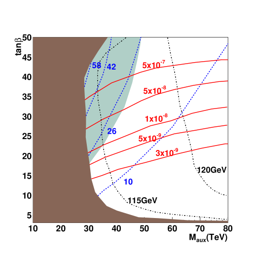
Figure 12: The contour plots for $a_{\mu}^{\rm SUSY}$ in unit of $10^{-10}$ (in the short dashed curves) and the Br ($B_{s}\rightarrow\mu^{+}\mu^{-}$) (in the solid curves) in the $(M_{\rm aux},\tan\beta)$ plane for the deflected AMSB scenarios with $M=10^{12}$ GeV, $N=6$, $\rho=0$ and $\mu>0$.

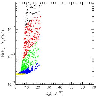
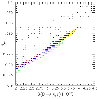
Figure 13: The correlations of (a) $Br(B_{s}\rightarrow\mu^{+}\mu^{-})$ with $a_{\mu}$, and (b) $Br(B\rightarrow X_{s}\gamma)$ with $R_{\mu\mu}$ in the deflected AMSB scenario with $M=10^{12}$ GeV, $N=6$, $\rho=0$ and $\mu>0$. The legends are the same as Fig. 2.

In Fig. 12, we show the contour plots in the $(M_{\rm aux},\tan\beta)$ plane with other parameters fixed to aforementioned values. In Figs. 13 (a) and (b), the correlations between (a) $R_{\mu\mu}$ and $B(B\rightarrow X_{s}\gamma)$ and (b) $B(B_{s}\rightarrow\mu^{+}\mu^{-})$ and $a_{\mu}$ in unit of $10^{-10}$ are shown. As expected, the sign flip of $M_{3}$ makes the model more consistent with $B\rightarrow X_{s}\gamma$. Note that the muon anomalous MDM cannot be greater than $22\times 10^{-10}$, and $0.93\leq R_{\mu\mu}\leq 1.10$. On the other hand, $B(B_{s}\rightarrow\mu^{+}\mu^{-})$ becomes as large as $\sim 10^{-6}$, because

III.6 Gaugino–assisted AMSB

In the line of minimal AMSB, eventually it is inevitable to clarify how one could generate the universal soft scalar mass squared $m_{0}^{2}$ put in the minimal AMSB by hand. The gaugino–assisted anomaly mediation (gAMSB) gives a simple origin of $m_{0}^{2}$ without additional fields or symmetries below the Planck scale gamsb . The setup is keeping the model of AMSB in its original form, but placing the MSSM gauge and gauginos in the bulk. Under the assumption of no singlet in the hidden sector boundary, the gauginos get masses via AMSB dominantly whereas scalar masses get contributions from both AMSB and a tiny hard breaking of SUSY by some operators on the hidden sector. These operators contribute to scalar masses at 1-loop, and being dominant in most of parameter space, and the tachyonic sleptons are cured. In this regard, it is a hybrid of gaugino mediation and anomaly mediation.

The soft terms at input scale are similar with mAMSB, but now the scalar masses get additional contribution which is not universal, but proportional to the matter gauge charges. Explicitly, we have

$$m^{2}=\tilde{m}^{2}+2\zeta(3)\Gamma(4)C(i)\frac{g^{2}}{16\pi^{2}}~{}{1\over(M_{*}L)^{2}}~{}m^{2}_{3/2}\,,$$ (36)

where $C(i)$ is the quadratic Casimir for the $i$ matter scalar representation, and the $\tilde{m}^{2}$ is the scalar masses in the pure AMSB scenario. The second term play the role of $m_{0}^{2}$ in the pure AMSB scenario where the tachyonic slepton problem is solved by adding $m_{0}^{2}$.

The parameter of the gaugino assisted AMSB scenario is the same as the mAMSB:

$$m_{3/2},~{}~{}~{}\eta,~{}~{}~{}\tan\beta,~{}~{}~{}{\rm sign}(\mu).$$

We scan over

$$3\leq\tan\beta\leq,~{}~{}~{}0\leq m_{3/2}\leq 100~{}{\rm TeV},~{}~{}~{}\eta=1,~{}~{}~{}\mu>0.$$

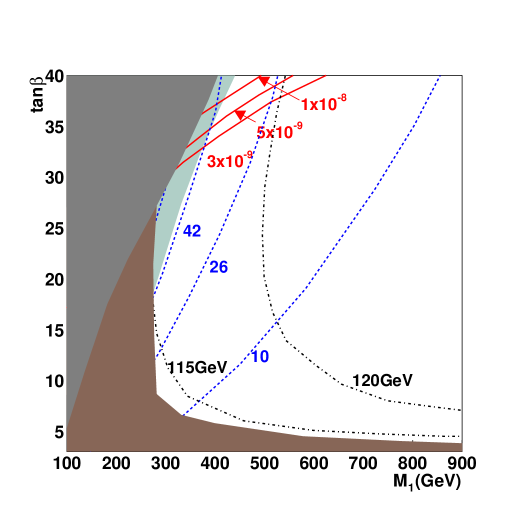
Figure 14: The contour plots for $a_{\mu}^{\rm SUSY}$ in unit of $10^{-10}$ (in the short dashed curves) and the Br ($B_{s}\rightarrow\mu^{+}\mu^{-}$) (in the solid curves) in the $(M_{1},\tan\beta)$ plane for the gaugino–assisted AMSB scenarios with $\mu>0$.

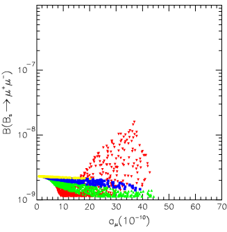
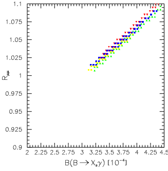
Figure 15: The correlations of (a) $Br(B_{s}\rightarrow\mu^{+}\mu^{-})$ with $a_{\mu}$, and (b) $Br(B\rightarrow X_{s}\gamma)$ with $R_{\mu\mu}$ in the gaugino-assisted AMSB scenario. The legends are the same as Fig. 2.

The qualitative features of the predictions in the gaugino-assisted AMSB scenario are similar to the mAMSB. $B\rightarrow X_{s}\gamma$ gives a strong constraint, especially for large $\tan\beta$. We find $B(B_{s}\rightarrow\mu^{+}\mu^{-})\lesssim 1.6\times 10^{-8}$ scanning over the parameter space. The results are depicted in Fig. 14 and Figs. 15 (a) and (b). The squark masses are generically large and their contributions to the decay $B_{s}\rightarrow\mu^{+}\mu^{-}$ is small. On the other hand, the charginos and the sleptons are relatively light and can contribute to $a_{\mu}$ up to $45\times 10^{-10}$. Finally we find $1.0\leq R_{\mu\mu}\leq 1.1$ and there is no large deviation from the SM prediction.

III.7 Weakly interacting string models with dilaton/moduli mediations

In the string theory, SUSY breaking is parametrized in terms of the nonzero values of the auxiliary components of dilaton and overall modulus superfields ($S$ and $T$, respectively) brignole :

$$F^{S} = \sqrt{3}(S+S^{*})m_{3/2}~{}\sin\theta,$$

$$F^{T} = \sqrt{3}(T+T^{*})m_{3/2}~{}\cos\theta.$$ (37)

Then universality of scalar fermion masses naturally follows in the dilaton dominated SUSY breaking mechanism. For weakly interacting heterotic string theories, the Kähler potential and the gauge kinetic function of the 4-dimensional low energy effective supergravity theory are given by brignole

$$K = -\ln(S+S^{*})-3\ln(T+T^{*})+(T+T^{*})^{n_{i}}\Phi_{i}\Phi_{i}^{*},$$

$$f_{ab} = {\delta_{ab}\over 4\pi}~{}S.$$ (38)

Here $n_{i}$ is the modular weight of the MSSM superfield $\Phi_{i}$. The soft terms at string scale can be derived from the above functions by well known formulae brignole . For $n_{i}=-1$ as an example, we have

$$M_{a}=\sqrt{3}M_{\rm aux}=-A_{ijk},~{}~{}~{}m_{ij}^{2}=M_{\rm aux}^{2}\delta_{ij}.$$ (39)

Here $M_{\rm aux}=m_{3/2}\sin\theta$ where $\theta$ is the Goldstino angle defined as $\tan\theta=F_{S}/F_{T}$. This model is specified by three independent parameters :

$$M_{\rm aux},~{}~{}~{}\tan\beta,~{}~{}~{}{\rm sign}(\mu).$$

Note that the Goldstino angle $\theta$ does not appear as an observable at this level.

In the dilaton domination scenario, one encounters the color charge breaking minima and the unbounded from below directions in the effective potential, if one starts the RG running from the usual GUT scale munoz ; casas ; abel . On the other hand, this problem can be evaded if one starts the RG running from the lower scale, for example, from the intermediate scale $M_{X}\sim 10^{11}$ GeV allanach . The detailed phenomenology on $a_{\mu}^{\rm SUSY}$, $B\rightarrow X_{s}\gamma$ and the neutralino-nucleus scattering in the limit of the dilaton domination has been already discussed by two of us in Ref. kolee both for $M_{\rm string}$ equal to the usual GUT scale and the intermediate string scale. In this work, we ignore the CCB and UFB problems and assume that the soft parameters are given at the conventional GUT scale $M_{\rm GUT}=2\times 10^{16}$ GeV, and will discuss other processes $B\rightarrow X_{s}l^{+}l^{-}$ and $B_{s}\rightarrow\mu^{+}\mu^{-}$. Earlier phenomenological analysis of weakly interacting string theories with dilaton domination scenarios can be found on the muon $(g-2)_{\mu}$ kchoi ; martin , $B\rightarrow X_{s}\gamma$. Discussions on $B\rightarrow X_{s}l^{+}l^{-}$ and $B_{s}\rightarrow\mu^{+}\mu^{-}$ in the weakly interacting string theories are given in this work for the first time.

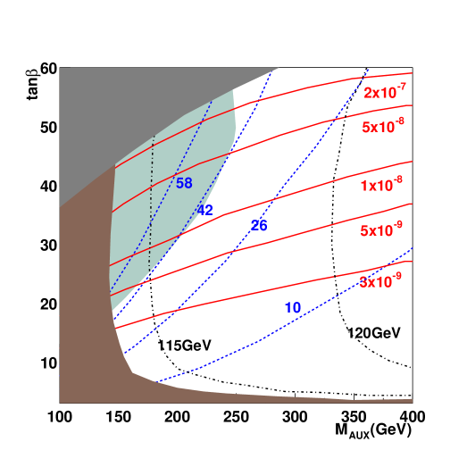
Figure 16: The contour plots for $a_{\mu}^{\rm SUSY}$ in unit of $10^{-10}$ (in the short dashed curves) and the Br ($B_{s}\rightarrow\mu^{+}\mu^{-}$) (in the solid curves) in the $(M_{\rm aux},\tan\beta)$ plane for the dilaton dominated scenario. The light gray region is excluded by the light stau mass bound, and the green region is excluded by the lower bound to the $B\rightarrow X_{s}\gamma$ branching ratio.

In Fig. 16, we show the constant contour plots for $a_{\mu}^{\rm SUSY}$ in unit of $10^{-10}$ (in the short dashed curves) and the Br ($B_{s}\rightarrow\mu^{+}\mu^{-}$) (in the solid curves) in the $(M_{\rm aux},\tan\beta)$ plane. In this scenario, the $a_{\mu}^{\rm SUSY}$ can be as large as $50\times 10^{-10}$ without any conflict with other constraints. The branching ratio for the decay $B_{s}\rightarrow\mu^{+}\mu^{-}$ can be as large as $2\times 10^{-7}$. Therefore the upcoming Tevatron Run II can probe a large portion of the parameter space of this scenario (down to $\tan\beta\sim 30$). We also find that $R_{\mu\mu}$ can vary between 0.95 and 1.15, which has a correlation with $B\rightarrow X_{s}\gamma$ similar to Fig. 2. Other comments are similar to the mSUGRA case.

III.8 Heterotic $M$ theory with dilaton/moduli mediations

Following the pioneering works of Witten and Horava and Witten horava , five different perturbative string theories are now regarded as different facets of one fundamental theory called $M$ theory, which describe the string theory in the strong coupling limit. The low energy limit of the $M$ theory is believed to be the 11-D SUGRA theory. Compactified on the orbifold $S^{1}/Z_{2}$ of the length $\pi\rho$ with two 10-dim. branes at the orbifold fixed points with two $E_{8}$ gauge groups living on each brane, this theory can accommodate the unification of three gauge coupling and Newton’s constant for gravity by adjusting the length of the 11-th dimensional orbifold. Further compactifying the 10-dim branes to 4 dimensional Minkowski space and Calabi-Yau or orbifolds with volume $V$, one can derive 4-dim low energy effective SUGRA from Horava-Witten theory. Note that there are three independent scales: $\kappa^{2}=M_{11}^{-9}$ (where $\kappa^{2}$ and $M_{11}$ being the Newton’s constant and the 11-dim. Planck constant), $\pi\rho$ (the length of the $S^{1}/Z_{2}$ orbifold interval) and $V$ (the volume of the 6-dim. internal space). There will be two model independent moduli superfields $S$ and $T$, whose scalar components satisfy

$${\rm Re}(S) = {1\over 2\pi(4\pi)^{2/3}}~{}M_{11}^{6}V,$$

$${\rm Re}(T) = {6^{1/3}\over 2(4\pi)^{4/3}}~{}M_{11}^{3}V^{1/3}\pi\rho.$$ (40)

In case there are more $T$ moduli, the scalar masses become nonuniversal in general, and SUSY flavor problem may get worse. The RG running effects involving the gluino mass parameter can mitigate this problem to some extent. In the following we take a simple framework in which the scalar mass term is universal from the outset. This assumption is well justified if we consider the compactified space is the Calabi-Yau manifold with Hodge-Betty number $h_{1,1}=1$.

For such strongly interacting string models (or M theories), the Kähler potential and the gauge kinetic function of the low energy effective supergravity theories are given by mtheory

$$K = -\ln(S+S^{*})-3\ln(T+T^{*})+\left({3\over T+T^{*}}+{\alpha\over S+S^{*}}\right)~{}\Phi_{i}\Phi_{i}^{*},$$

$$f_{ab} = {\delta_{ab}\over 4\pi}~{}(S+\alpha T).$$ (41)

The soft terms at the string scale are derived from the above functions as follows ckm :

$$M_{a} = {\sqrt{3}m_{3/2}\over 1+\epsilon}~{}\left[\sin\theta+{\epsilon\over\sqrt{3}}\cos\theta\right],$$

$$A_{ijk} = -{\sqrt{3}m_{3/2}\over 3+\epsilon}~{}\left[(3-2\epsilon)\sin\theta+\sqrt{3}\epsilon\cos\theta\right],$$

$$m_{ij}^{2} = m_{3/2}^{2}\delta_{ij}\left[1-{3\over(3+\epsilon)^{2}}~{}\left(\epsilon(6+\epsilon)\sin^{2}\theta+(3+2\epsilon)\cos^{2}\theta-2\sqrt{3}\epsilon\sin\theta\cos\theta\right)\right].$$ (42)

Here $\theta$ is the Goldstino angle as before, and

$$\epsilon\equiv\alpha(T+T^{*})/(S+S^{*}).$$

Therefore there are five independent input parameters in the heterotic $M$ theory :

$$m_{3/2},~{}~{}~{}\sin\theta,~{}~{}~{}\epsilon,~{}~{}~{}\tan\beta,~{}~{}~{}{\rm sign}(\mu).$$

Note that the universality in the scalar masses and gaugino masses as well as trilinear couplings are realized in this scenario, which are functions of the Goldstino angle $\theta$ and the parameter $\epsilon$. In most parameter space, one has $M_{a}^{2}>m_{ij}^{2}$ at the string scale. In the heterotic $M$ theory, one recovers the dilaton domination scenario in the limit of $\epsilon\rightarrow 0$, namely $(T+T^{*})<<(S+S^{*})$. The parameter $\epsilon$ lies in the range $0<\epsilon<1$ for the standard embedding of the spin connection, but it can take a negative value for the nonstandard embedding. For the latter the gaugino mass is even larger than the scalar masses. Overall phenomenology of this scenario for low energy processes is more or less the same as the mSUGRA or the dilaton domination scenarios. Let us make a comment that the problem of CCB and UFB are solved in this scenario in a wide region of parameter space $\epsilon$ and $\theta$ mtheory .

Let us make two comments on the phenomenological niceties of the heterotic $M$ theory compared to the weakly interacting heterotic string theory other than the unification of the gauge coupling and Newton’s constant:

• Although we do not care about the CCB and the UFB problems in this work, it is worthwhile to note that the case with $0<\epsilon<1$ (the standard embedding) has the CCB and UFB problems and there is no parameter space left if the top mass is to be reproduced, whereas the nonstandard embedding (for which $-1<\epsilon<0$) has no such a problem.

• The limit $\theta\rightarrow 0$ exists in the heterotic $M$ theory (except for $\epsilon=0$) with soft masses remaining finite, all of which are order of $\epsilon~{}m_{3/2}$. On the other hand, the soft terms in the weakly interacting heterotic string theory considered in the previous subsection vanish in the limit $\theta\rightarrow 0$. Therefore one has to include the string one loop corrections or the sigma model one loop corrections to the Kähler potential and the gauge kinetic function.

Note that this scenario is a special case of mSUGRA scenario except that the gaugino mass parameter can change the sign depending on $\epsilon$ and $\theta$. Earlier phenomenological analysis of heterotic $M$ theories can be found on the muon $(g-2)_{\mu}$ kchoi ; cerdeno , $B\rightarrow X_{s}\gamma$ Huang:1998tn ; kchoi , and and $B\rightarrow X_{s}\tau^{+}\tau^{-}$ Huang:1998tn . The discussion on $B_{s}\rightarrow\mu^{+}\mu^{-}$ in the heterotic $M$ theories is given in this work for the first time.

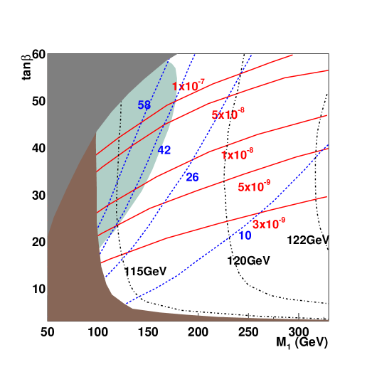
Figure 17: The contour plots for $a_{\mu}^{\rm SUSY}$ in unit of $10^{-10}$ (in the short dashed curves) and the Br ($B_{s}\rightarrow\mu^{+}\mu^{-}$) (in the solid curves) in the $(M_{1},\tan\beta)$ plane for the heterotic M theory with $\epsilon=+0.5$ and $\theta=0.15\pi$.

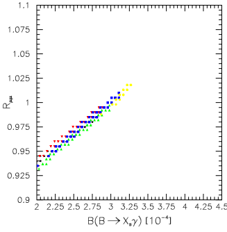
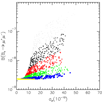
Figure 18: The correlations of the $Br(B\rightarrow X_{s}\gamma)$ with (a) $R_{\mu\mu}$, and (b) $a_{\mu}^{\rm SUSY}$ for the heterotic M theory with $\epsilon=+0.5$ and $\theta=0.15\pi$. The legends are the same as Fig. 2.

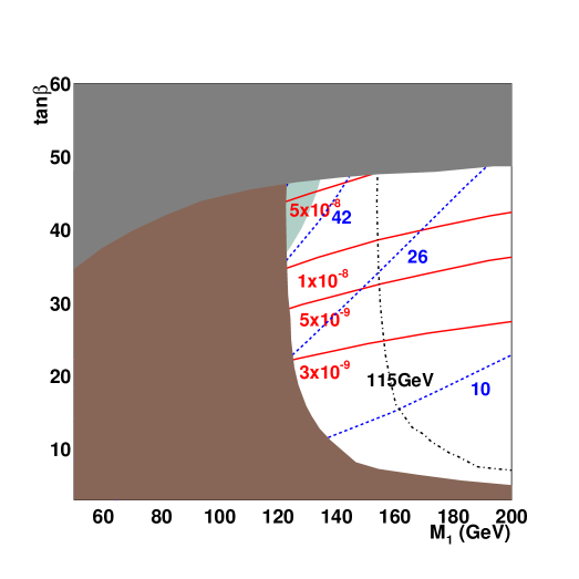
Figure 19: The contour plots for $a_{\mu}^{\rm SUSY}$ in unit of $10^{-10}$ (in the short dashed curves) and the Br ($B_{s}\rightarrow\mu^{+}\mu^{-}$) (in the solid curves) in the $(M_{1},\tan\beta)$ plane for the heterotic M theory with $\epsilon=-0.8$ and $\theta=0.15\pi$.

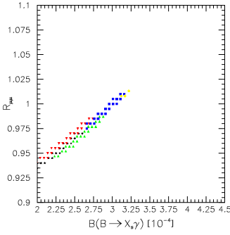
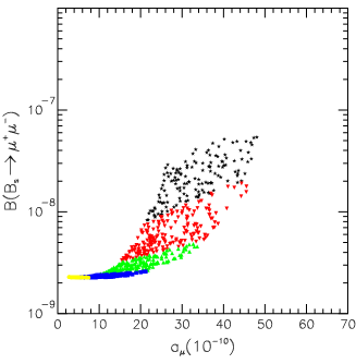
Figure 20: The correlations of the $Br(B\rightarrow X_{s}\gamma)$ with (a) $R_{\mu\mu}$, and (b) $a_{\mu}^{\rm SUSY}$ for the heterotic M theory with $\epsilon=-0.8$ and $\theta=0.15\pi$. The legends are the same as Fig. 2.

In the heterotic $M$ theory, the universal gaugino mass $M_{a}$ is dominant over the common scalar mass $|m_{ij}|$ at the messenger scale. Then at the electroweak scale, $m_{\tilde{\tau}}^{2}<0$ in most region of parameter space for large $\tan\beta$ except for very narrow range of $\epsilon$ and $\theta$. Also, for $\theta>\pi$, the gaugino mass parameter changes its sign as in the AMSB scenario, and the HRS effect comes into play for positive $\mu$. With this general comment in mind, we fix $\theta=0.15\pi$ and show the contour plots for $\epsilon=+0.5$ and $-0.8$ in the $(M_{1},\tan\beta)$ plane, and various correlations in Figs. 17–20. Note that the common gaugino mass parameter $M_{a}$ can be negative altogether for certain range of $\theta$ for a fixed $\epsilon$. Then the situation would be similar to the AMSB scenario where $M_{3}<0$. However, in the heterotic $M$ theory, all the three gaugino mass parameter changes the signs unlike the AMSB case where only $M_{3}$ change its sign. Therefore, $a_{\mu}^{\rm SUSY}>0$ implies $\mu M_{2}>0$ and $B\rightarrow X_{s}\gamma$ prefers $\mu M_{3}>0$. There is no problem with satisfying both constraints if we flip the sign of $\mu$ for negative gaugino mass parameter.

III.9 $D$ brane models

Advances in understanding the role of $D-$branes in superstring theories brought new ideas in particle physics model buildings. Several attempts have been made to obtain (semi)realistic 4-dimensional models (SM, MSSM or their variations) ibanez ; dbrane . SM gauge groups and matters can be put on the same or different branes, according to which the patterns of the resulting soft SUSY breaking terms can differ. In this subsection, we choose a specific $D$ brane model where the SM gauge groups and 3 generations live on different $Dp$ branes dbrane . In this model, scalar fermion masses are not completely universal and gaugino mass unification can be relaxed. Also the string scale is around $10^{12}$ GeV (the intermediate scale) rather than GUT scale.

Since there are now three moduli ($T_{i}$) fields and one dilaton superfield in this scenario, we modify the parametrization appropriate for several $T_{i}$ moduli as follows:

$$F^{S} = \sqrt{3}~{}(S+S^{*})~{}m_{3/2}\sin\theta,$$

$$F^{i} = \sqrt{3}~{}(T_{i}+T_{i}^{*})~{}m_{3/2}\cos\theta~{}\Theta_{i}$$ (43)

where $\theta$ and $\Theta_{i}~{}(i=1,2,3)$ with $|\Theta_{i}|^{2}=1$ parametrize the directions of the goldstinos in the $S,T_{i}$ field space. Then, the gaugino masses are given by

$$M_{3} = \sqrt{3}m_{3/2}\sin\theta,$$

$$M_{2} = \sqrt{3}m_{3/2}\Theta_{1}\cos\theta,$$

$$M_{Y} = \sqrt{3}m_{3/2}\alpha_{Y}(M_{I})~{}\left({2\Theta_{3}\cos\theta\over\alpha_{1}(M_{I})}+{\Theta_{1}\cos\theta\over\alpha_{2}(M_{I})}+{2\sin\theta\over 3\alpha_{3}(M_{I})}\right),$$ (44)

where

$${1\over\alpha_{Y}(M_{I})}={2\over\alpha_{1}(M_{I})}+{1\over\alpha_{2}(M_{I})}+{2\over 3\alpha_{3}(M_{I})}.$$ (45)

The string scale $M_{I}$ is determined to be $M_{I}=10^{12}~{}(5\times 10^{14})$ GeV from the $U(1)_{1}$ gauge coupling $\alpha_{1}(M_{I})=0.1(1)$ dbrane . Note that the gaugino masses are non universal in a natural way in this scenario, unlike other scenarios studied in the previous subsections.

The soft masses for the sfermions and Higgs fields are given by

$$m_{Q}^{2} = m_{3/2}^{2}~{}\left[~{}1-{3\over 2}\left(1-\Theta_{1}^{2}\right)~{}\cos^{2}\theta~{}\right],$$

$$m_{u^{c}}^{2} = m_{3/2}^{2}~{}\left[~{}1-{3\over 2}\left(1-\Theta_{3}^{2}\right)~{}\cos^{2}\theta~{}\right],$$

$$m_{d^{c}}^{2} = m_{3/2}^{2}~{}\left[~{}1-{3\over 2}\left(1-\Theta_{2}^{2}\right)~{}\cos^{2}\theta~{}\right],$$

$$m_{L}^{2} = m_{3/2}^{2}~{}\left[~{}1-{3\over 2}\left(\sin^{2}\theta+\Theta_{3}^{2}~{}\cos^{2}\theta\right)\right],$$

$$m_{e^{c}}^{2} = m_{3/2}^{2}~{}\left[~{}1-{3\over 2}\left(\sin^{2}\theta+\Theta_{1}^{2}~{}\cos^{2}\theta\right)\right],$$

$$m_{H_{2}}^{2} = m_{3/2}^{2}~{}\left[~{}1-{3\over 2}\left(\sin^{2}\theta+\Theta_{2}^{2}~{}\cos^{2}\theta\right)\right],$$

$$m_{H_{1}}^{2} = m_{L}^{2}.$$ (46)

Note that the scalar mass universality in the sfermion masses and Higgs masses is achieved when

$$\sin^{2}\theta={1\over 4}~{}~{}~{}{\rm and}~{}~{}~{}\Theta_{i}^{2}={1\over 3}~{}~{}~{}{\rm for}~{}i=1,2,3.$$ (47)

And in this case the gaugino masses becomes also universal, when we take only positive numbers for the solutions. For other choices of goldstino angles, the scalar and the gaugino masses become nonuniversal, and there could be larger flavor violations in the low energy processes as well as enhanced SUSY contributions to the $a_{\mu}^{\rm SUSY}$.

The trilinear couplings are given by

$$A_{u} = {\sqrt{3}\over 2}~{}m_{3/2}~{}\left[(\Theta_{2}-\Theta_{1}-\Theta_{3})\cos\theta-\sin\theta\right],$$

$$A_{d} = {\sqrt{3}\over 2}~{}m_{3/2}~{}\left[(\Theta_{3}-\Theta_{1}-\Theta_{2})\cos\theta-\sin\theta\right],$$

$$A_{e} = 0.$$ (48)

Therefore the $D$ brane model we consider in this work is specified by following six parameters :

$$m_{3/2},~{}~{}\tan\beta,~{}~{}\theta,~{}~{}\Theta_{i=1,2},~{}~{}{\rm sign}(\mu).$$

Earlier phenomenological analysis of $D$ brane models can be found on the muon $(g-2)_{\mu}$ munoz2 .The discussion on $B\rightarrow X_{s}\gamma$, $B\rightarrow X_{s}l^{+}l^{-}$ and $B_{s}\rightarrow\mu^{+}\mu^{-}$ in this scenario is given in the present work for the first time.

For numerical analysis, we fix $\Theta_{i}=+1/\sqrt{3}$ for all $i=1,2,3$, (the overall modulus limit) and we scan over the following parameter space : $-\pi/4\leq\theta\leq 4/\pi$, $m_{3/2}\leq 300$ GeV, and $\tan\beta\leq 50$. In this case, the universality in sfermion and Higgs masses parameters at the string scale is moderately broken. Still there remain certain degrees of degeneracy: the squark masses are universal at string scale $M_{I}$, the sleptons and the down type Higgs ($H_{2}$) masses are the same, and the up type ($H_{1}$) Higgs are degenerate. The gaugino masses are nonuniversal for this choice of parameters. The point corresponding to the universality in the scalar and gaugino masses is denoted by the filled triangle. Another interesting aspect of this model is that the gluino mass parameter $M_{3}$ can have either sign for $-\pi/4<\theta<0$ as in the AMSB model, and the correlation between $a_{\mu}^{\rm SUSY}$ and $B\rightarrow X_{s}\gamma$ resembles that of the AMSB scenario.

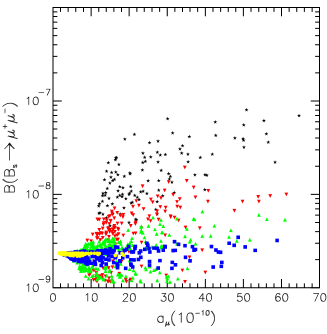
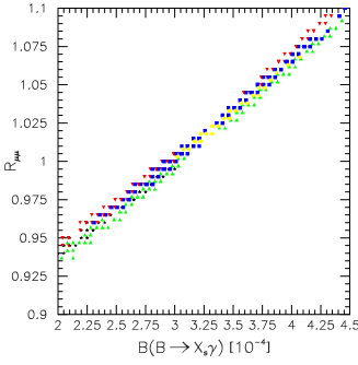
Figure 21: The correlations between (a) $a_{\mu}^{\rm SUSY}$ and $B(B_{s}\rightarrow\mu^{+}\mu^{-})$, and (b) $R_{\mu\mu}$ and $B(B\rightarrow X_{s}\gamma)$ in the $D-$brane model considered in Sec. III G. We fix $\Theta_{i}=1/\sqrt{3}$ for all $i=1,2,3$, (the overall modulus limit) and we scan over the following parameter space : $-\pi/4\leq\theta\leq 4/\pi$, $m_{3/2}\leq 300$ GeV, and $\tan\beta\leq 50$.

In Figs. 21 (a) and (b), we show the correlations between (a) $a_{\mu}^{\rm SUSY}$ and $B(B_{s}\rightarrow\mu^{+}\mu^{-})$ and (b) $R_{\mu\mu}$ and $B(B\rightarrow X_{s}\gamma)$, respectively. Both $a_{\mu}^{\rm SUSY}$ and $B(B_{s}\rightarrow\mu^{+}\mu^{-})$ can be large for large $\tan\beta$, as in the mSUGRA. In particular, $a_{\mu}^{\rm SUSY}$ can be as large as $70\times 10^{-10}$, unlike the minimal SUGRA model with $m_{0}=300$ GeV for which $a_{\mu}^{\rm SUSY}$ is limited only to $32\times 10^{-10}$. Also $B(B_{s}\rightarrow\mu^{+}\mu^{-})>2\times 10^{-8}$ is possible in an ample region of the parameter space as in the mSUGRA. The fact that $M_{3}$ can change its sign shows itself in the correlation in Fig. 21 (b). $R_{\mu\mu}$ can either decrease down to 0.86 or increase up to 1.15, depending on the sign of $M_{3}$. Still the deviation from the SM is not significant, and it would not be easy to observe this effect from $R_{\mu\mu}$.

On the other hand, one may assume that all the SM gauge groups are embedded within the same set of $D_{p}$ branes dbrane . For this case, a salient feature is that there appear Higgs doublets $H_{1}^{i}$ and $H_{2}^{i}$ come in three generations. Therefore there could be large FCNC contributions due to scalar exchanges, unless one removes flavor changing neutral current interactions by imposing some discrete symmetry. Although the soft terms for these models are known, it is too premature to study the detailed phenomenology of this class of models, before we know well enough how to handle this flavor changing scalar interactions.

IV Conclusions

In conclusion, we considered four low energy processes $(g-2)_{\mu}$, $B\rightarrow X_{s}\gamma$, $B\rightarrow X_{s}l^{+}l^{-}$ and $B_{s}\rightarrow\mu^{+}\mu^{-}$ in various models for SUSY breaking mediation mechanisms which are theoretically well motivated. Since many models predict universal scalar masses at the messenger scale, the RG running induces very important features for the stop mass and the $A_{t}$ parameter depending on the location of the messenger scale. If the messenger scale is high around GUT scale, then the lower bound on the $B\rightarrow X_{s}\gamma$ branching ratio is constraining for the $\mu>0$ case, because the chargino-stop loop contribution interfere destructively with the SM and the charged Higgs contributions (except for the AMSB scenario). The $A_{t}$ term relevant to the stop-chargino loop contribution is generated mainly by the gluino loop by RG running effects. On the other hand, in the GMSB scenario with low messenger scales ($M_{\rm mess}\sim 10^{6}$ GeV or so), the stop mass is relatively heavy, and the $A_{t}$ parameter is very small so that the stop - chargino contribution to $B\rightarrow X_{s}\gamma$ is negligible. This is the reason why the $B_{s}\rightarrow\mu^{+}\mu^{-}$ branching ratio is much suppressed in the GMSB with low $M_{\rm mess}$ and $N_{\rm mess}$. This decay is also suppressed in the AMSB scenario because the stop is relatively heavy in this scenario. In fact, the branching ratio for $B_{s}\rightarrow\mu^{+}\mu^{-}$ cannot be larger than $2\times 10^{-8}$ for these low messenger scale GMSB scenarios with $N_{\rm mess}=1$ or in the AMSB scenario. On the other hand, its branching ratio can be much larger for mSUGRA or string inspired models where the messenger scale is around the GUT scale. The Tevatron Run II can probe the $B_{s}\rightarrow\mu^{+}\mu^{-}$ decay mode down to $\sim 2\times 10^{-8}$ level in the branching ratio. Therefore if $B_{s}\rightarrow\mu^{+}\mu^{-}$ is discovered at the Tevatron Run II, then the AMSB or the GMSB with small $N_{\rm mess}$ will be definitely excluded independent of the direct searches of SUSY particles. With the new lower limits on Higgs (and SUSY particles), there is little chance to expect large deviations in $R_{\mu\mu}$ from its SM prediction $R_{\mu\mu}=1$. If any significant deviation in $R_{\mu\mu}$ is observed at $B$ factories, it would reject all the SUSY breaking mediation scenarios we have considered in this work.

Note Added

While this work is being finished, a new result on the muon $(g-2)$ was reported by BNL Muon $(g-2)$ Collaboration bnl02 , and a few related works nath02 ; davier02 thereafter. The new result implies that davier02

$$a_{\mu}^{\rm exp}-a_{\mu}^{\rm SM}=33.9(11.2)~{}~{}{\rm to}~{}~{}16.7(10.7)\times 10^{-10}\equiv a_{\mu}^{\rm SUSY},$$

depending on how the hadronic contributions are treated: the first and the second numbers are based on the $e^{+}e^{-}\rightarrow hadrons$ and the hadronic $\tau$ decays, respectively. Another calculation by Hagiwara et al. hagiwara also indicates that the SM prediction is 2.7 $\sigma$ below the experimental value. This new data do not affect the conclusons of the present work very much. In particular, there is still a possibility that the $B_{s}\rightarrow\mu^{+}\mu^{-}$ branching ratio can be large enough to be found at the Tevatron Run II, if we allow the $3\sigma$ range for the $a_{\mu}^{\rm SUSY}$ (see Fig, 2 (a), for example).

References

- (1) For reviews, see H. P. Nilles, Phys. Rep. 150, 1 (1984); H. E. Haber and G. Kane, ibid. 117, 75 (1985).
- (2) H. P. Nilles, Phys. Lett. B 115 (1982) 193; Nucl. Phys. B 217 (1983) 366; A. Chamseddine, R. Arnowitt, P. Nath, Phys. Rev. Lett. 49 (1982) 970; R. Barbieri, S. Ferrara, C. Savoy, Phys. Lett. B 119 (1982) 343; L. Hall, J. Lykken, S. Weinberg, Phys. Rev. D 27 (1983) 2359; S. K. Soni, H. A. Weldon, Phys. Lett. B 126 (1983) 215.
- (3) M. Dine and A. E. Nelson, Phys. Rev. D 48, 1277 (1993); M. Dine, A. E. Nelson, Y. Nir and Y. Shirman, ibid., 53, 2658; for a review, see G. F. Giudice and R. Rattazzi, Phys. Rep. 322, 419 (1999).
- (4) L. Randall and R. Sundrum, Nucl. Phys. B 557, 79 (1999); G. F. Giudice, M. A. Luty, H. Murayama and R. Rattazzi, JHEP 9812, 027 (1998); T. Gherghetta, G. F. Giudice and J. D. Wells, Nucl. Phys. B 559, 27 (1999).
- (5) Z. Chacko, M. A. Luty and E. Ponton, JHEP 0007, 036 (2000); D. E. Kaplan, G. D. Kribs and M. Schmaltz, Phys. Rev. D 62, 035010 (2000); Z. Chacko, M. A. Luty, A. E. Nelson and E. Ponton, JHEP 0001, 003 (2000).
- (6) For a review, see A. B. Lahanas and D. V. Nanopoulos, Phys. Rep. 145, 1 (1987).
- (7) L. J. Hall, R. Rattazzi and U. Sarid, Phys. Rev. D 50, 7048 (1994)
- (8) H. E. Logan, Nucl. Phys. Proc. Suppl. 101, 279 (2001), and references therein.
- (9) S. Baek, P. Ko and W. Y. Song, Phys. Rev. Lett. 89, 271801 (2002) [arXiv:hep-ph/0205259].
- (10) A. Dedes, H. K. Dreiner and U. Nierste, Phys. Rev. Lett. 87, 251804 (2001).
- (11) K. Choi, K. Hwang, S. K. Kang, K. Y. Lee and W. Y. Song, Phys. Rev. D 64, 055001 (2001) [arXiv:hep-ph/0103048].
- (12) H. Baer, C. Balazs, J. Ferrandis and X. Tata, Phys. Rev. D 64, 035004 (2001) [arXiv:hep-ph/0103280]; A. Dedes, H. K. Dreiner, U. Nierste and P. Richardson, [arXiv:hep-ph/0207026].
- (13) L. L. Everett, G. L. Kane, S. Rigolin and L. T. Wang, Phys. Rev. Lett. 86, 3484 (2001) [arXiv:hep-ph/0102145]; J. L. Feng and K. T. Matchev, Phys. Rev. Lett. 86, 3480 (2001) [arXiv:hep-ph/0102146]; E. A. Baltz and P. Gondolo, Phys. Rev. Lett. 86, 5004 (2001) [arXiv:hep-ph/0102147]; U. Chattopadhyay and P. Nath, Phys. Rev. Lett. 86, 5854 (2001) [arXiv:hep-ph/0102157]; S. Komine, T. Moroi and M. Yamaguchi, Phys. Lett. B 506, 93 (2001) [arXiv:hep-ph/0102204]. J. R. Ellis, D. V. Nanopoulos and K. A. Olive, Phys. Lett. B 508, 65 (2001) [arXiv:hep-ph/0102331]; M. Byrne, C. F. Kolda and J. E. Lennon, arXiv:hep-ph/0108122.
- (14) S. Ambrosanio, A. Dedes, S. Heinemeyer, S. Su and G. Weiglein, Nucl. Phys. B 624, 3 (2002) [arXiv:hep-ph/0106255].
- (15) M. Knecht and A. Nyffeler, Phys. Rev. D 65, 073034 (2002); M. Knecht, A. Nyffeler, M. Perrottet, and E. de Rafael, Phys. Rev. Lett. 88, 071802 (2002); M. Hayakawa and T. Kinoshita, arXiv:hep-ph/0112102; A. Czarnecki, and K. Melnikov, Phys. Rev. Lett. 88, 071803 (2002), J. Bijnens, E. Pallante, and J. Prades, Nucl. Phys. B626 410 (2002).
- (16) S. P. Martin and J. D. Wells, Phys. Rev. D 64, 035003 (2001)
- (17) H. N. Brown et al., Phys. Rev. Lett. 86, 2227 (2001).
- (18) G. C. Cho, N. Haba and J. Hisano, Phys. Lett. B 529, 117 (2002); S. Baek, P. Ko and J. H. Park, arXiv:hep-ph/0203251.
- (19) L. Wolfenstein, Phys. Rev. Lett. 51, 1945 (1983).
- (20) A. L. Kagan and M. Neubert, Eur. Phys. J. C 7, 5 (1999) [arXiv:hep-ph/9805303].
- (21) BELLE Collaboration, arXiv:hep-ex/0111037, Contributed to the Proceedings of the XX International Symposium on Lepton and Photon Interactions at High Energies, July 23–28, 2001, Rome, Italy.
- (22) S. Chen et al., CLEO Collaboration, Phys. Rev. Lett. 87, 251807 (2001).
- (23) A.L. Kagan and M. Neubert, Eur. Phys. J. C 7, 5 (1999).
- (24) A.J. Buras, A. Czarnecki, M. Misiak, and J. Urban, arXiv:hep-ph/0203135; A.J. Buras, A. Czarnecki, M. Misiak, and J. Urban, Nucl. Phys. B611, 488 (2001); P. Gambino and M. Misiak, Nucl. Phys. B611, 338 (2001); K. Chetyrkin, M. Misiak, and M. Mnz, Phys. Lett. B 400, 206 (1997); Erratum ibid B 425, 414 (1998); C. Greub, T. Hurth, and D. Wyler, Phys. Rev. D 54, 3350 (1996); A. J. Buras, A. Czarnecki, M. Misiak and J. Urban, Nucl. Phys. B 631, 219 (2002) [arXiv:hep-ph/0203135].
- (25) Y. B. Dai, C. S. Huang and H. W. Huang, Phys. Lett. B 390, 257 (1997) [Erratum-ibid. B 513, 429 (2001)] [arXiv:hep-ph/9607389].
- (26) T. Goto, Y. Okada and Y. Shimizu, Phys. Rev. D 58, 094006 (1998) [arXiv:hep-ph/9804294].
- (27) E. Gabrielli and U. Sarid, Phys. Rev. Lett. 79, 4752 (1997) [arXiv:hep-ph/9707546] ; Phys. Rev. D 58, 115003 (1998) [arXiv:hep-ph/9803451].
- (28) S. Baek and P. Ko, Phys. Lett. B 462, 95 (1999) [arXiv:hep-ph/9904283]; E. Lunghi, A. Masiero, I. Scimemi and L. Silvestrini, Nucl. Phys. B 568, 120 (2000) [arXiv:hep-ph/9906286]; A. Ali and E. Lunghi, Eur. Phys. J. C 21, 683 (2001) [arXiv:hep-ph/0105200].
- (29) A. J. Buras and M. Munz, Phys. Rev. D 52, 186 (1995) [arXiv:hep-ph/9501281]; K. G. Chetyrkin, M. Misiak and M. Munz, Phys. Lett. B 400, 206 (1997) [Erratum-ibid. B 425, 414 (1998)] [arXiv:hep-ph/9612313]; A. Ali and G. Hiller, Phys. Rev. D 60, 034017 (1999) [arXiv:hep-ph/9807418]; A. Ali and G. Hiller, Eur. Phys. J. C 8, 619 (1999) [arXiv:hep-ph/9812267].
- (30) K. Abe et al. [Belle Collaboration], arXiv:hep-ex/0107072; K. Abe et al. [BELLE Collaboration], Phys. Rev. Lett. 88, 021801 (2002) [arXiv:hep-ex/0109026]; B. Aubert et al. [BABAR Collaboration], arXiv:hep-ex/0107026.
- (31) A. Ali, P. Ball, L. T. Handoko and G. Hiller, Phys. Rev. D 61, 074024 (2000) [arXiv:hep-ph/9910221].
- (32) CDF Collaboration, F. Abe et al., Phys. Rev. D 57, 3811 (1998)
- (33) R. Arnowitt, B. Dutta, T. Kamon and M. Tanaka, arXiv:hep-ph/0203069.
- (34) C. Huang, W. Liao and Q. Yan, Phys. Rev. D 59 (1999) 011701, arXiv:hep-ph/9803460.
- (35) S. R. Choudhury and N. Gaur, Phys. Lett. B 451, 86 (1999) [arXiv:hep-ph/9810307]; S. Rai Choudhury, A. Gupta and N. Gaur, Phys. Rev. D 60, 115004 (1999) [arXiv:hep-ph/9902355].
- (36) K. S. Babu and C. Kolda, Phys. Rev. Lett. 84, 228 (2000), arXiv:hep-ph/9909476.
- (37) C. S. Huang, W. Liao, Q. S. Yan and S. H. Zhu, Phys. Rev. D 63, 114021 (2001) [Erratum-ibid. D 64, 059902 (2001)] [arXiv:hep-ph/0006250]; C. S. Huang and X. H. Wu, arXiv:hep-ph/0212220.
- (38) P. H. Chankowski and L. Slawianowska, Phys. Rev. D 63, 054012 (2001), arXiv:hep-ph/0008046.
- (39) C. Bobeth, T. Ewerth, F. Kruger and J. Urban, Phys. Rev. D 64 074014 (2001), arXiv:hep-ph/0104284.
- (40) M. Carena, D. Garcia, U. Nierste, and C. E. M. Wagner, Nucl. Phys. B577, 88 (2000), arXiv:hep-ph/9912516.
- (41) G. Isidori and A. Retico, JHEP 0111, 001 (2001) [arXiv:hep-ph/0110121]; G. Isidori and A. Retico, JHEP 0209, 063 (2002) [arXiv:hep-ph/0208159].
- (42) T. Ibrahim and P. Nath, Phys. Rev. D 67, 016005 (2003) [arXiv:hep-ph/0208142]; A. Dedes and A. Pilaftsis, Phys. Rev. D 67, 015012 (2003) [arXiv:hep-ph/0209306].
- (43) J. A. Casas, A. Lleyda, and C. Munoz, Nucl. Phys. B471 3 (1996); H. Baer, M. Brhlik, and D. Castano, Phys. Rev. D 54, 6944 (1996).
- (44) J. A. Casas, A. Lleyda, and C. Munoz, Phys. Lett. B380, 59 (1996).
- (45) S. A. Abel and C. Savoy, Phys. Lett. B444, 119 (1998); J. A. Casas, A. Ibarra, and C. Munoz, Nucl. Phys. B554, 67 (1999).
- (46) K. T. Mahanthappa and S. Oh, Phys. Rev. D 62, 015012 (2000) [arXiv:hep-ph/9908531].
- (47) J. L. Feng and T. Moroi, Phys. Rev. D 61, 095004 (2000) [arXiv:hep-ph/9907319]. See also Refs. kchoi and tata .
- (48) A. Anisimov, M. Dine, M. Graesser, S. Thomas, Phys. Rev. D 65 105011 (2002); ibid, arXive:hep-th/0201256.
- (49) R. Harnik, H. Murayama, A. Pierce, arXiv:hep-ph/0204122.
- (50) S. Komine and M. Yamaguchi, Phys. Rev. D 63 035005 (2001), arXiv:hep-ph/0007327. S. Komine, T. Moroi and M. Yamaguchi, Phys. Lett. B 507, 224 (2001) [arXiv:hep-ph/0103182].
- (51) A. Pomarol and R. Rattazzi, JHEP 9905, 013 (1999) [arXiv:hep-ph/9903448]; R. Rattazzi, A. Strumia and J. D. Wells, Nucl. Phys. B 576, 3 (2000) [arXiv:hep-ph/9912390].
- (52) D. E. Kaplan and G. D. Kribs, JHEP 0009, 048 (2000) [arXiv:hep-ph/0009195].
- (53) N. Arkani-Hamed, D. E. Kaplan, H. Murayama and Y. Nomura, JHEP 0102, 041 (2001) [arXiv:hep-ph/0012103].
- (54) A. Brignole, L. E. Ibanez and C. Munoz, Nucl. Phys. B 422, 125 (1994) [Erratum-ibid. B 436, 747 (1995)] [arXiv:hep-ph/9308271]; A. Brignole, L. E. Ibanez, C. Munoz and C. Scheich, Z. Phys. C 74, 157 (1997) [arXiv:hep-ph/9508258].
- (55) S. A. Abel, B. C. Allanach, F. Quevedo, L. Ibanez and M. Klein, JHEP 0012, 026 (2000) [arXiv:hep-ph/0005260].
- (56) S. Baek, P. Ko and H. S. Lee, Phys. Rev. D 65, 035004 (2002) [arXiv:hep-ph/0103218].
- (57) P. Horava and E. Witten, Nucl. Phys. B 460, 506 (1996) [arXiv:hep-th/9510209]; Nucl. Phys. B 475, 94 (1996) [arXiv:hep-th/9603142].
- (58) C. Munoz, arXiv:hep-th/9906152; H. P. Nilles, arXiv:hep-ph/0004064, and references therein.
- (59) K. Choi, H. B. Kim and C. Munoz, Phys. Rev. D 57, 7521 (1998) [arXiv:hep-th/9711158]; A. Lukas, B. A. Ovrut and D. Waldram, Phys. Rev. D 57, 7529 (1998) [arXiv:hep-th/9711197].
- (60) D. G. Cerdeno and C. Munoz, Phys. Rev. D 66, 115007 (2002) [arXiv:hep-ph/0206299].
- (61) C. S. Huang, T. j. Li, W. Liao, Q. S. Yan and S. H. Zhu, Eur. Phys. J. C 18, 393 (2000) [arXiv:hep-ph/9810412].
- (62) G. Aldazabal, L. E. Ibanez and F. Quevedo, JHEP 0001, 031 (2000) [arXiv:hep-th/9909172]; G. Aldazabal, L. E. Ibanez and F. Quevedo, JHEP 0002, 015 (2000) [arXiv:hep-ph/0001083]; G. Aldazabal, L. E. Ibanez, F. Quevedo and A. M. Uranga, JHEP 0008, 002 (2000) [arXiv:hep-th/0005067].
- (63) D. G. Cerdeno, E. Gabrielli, S. Khalil, C. Munoz, and E. Torrente-Lujan, Nucl. Phys. B 603, 231 (2001) [arXiv:hep-ph/0102270].
- (64) D. G. Cerdeno, E. Gabrielli, S. Khalil, C. Munoz and E. Torrente-Lujan, Phys. Rev. D 64, 093012 (2001) [arXiv:hep-ph/0104242]; See also Ref. kolee .
- (65) G. W. Bennett [Muon g-2 Collaboration], arXiv:hep-ex/0208001.
- (66) E. A. Baltz and P. Gondolo, arXiv:astro-ph/0207673; U. Chattopadhyay and P. Nath, arXiv:hep-ph/0208012; M. Byrne, C. Kolda, J. E. Lennon, arXiv:hep-ph/0208067; Yeong Gyun Kim, Takeshi Nihei, Leszek Roszkowski, Roberto Ruiz de Austri, arXiv:hep-ph/0208069; J. K. Mizukoshi, X. Tata and Y. Wang, Phys. Rev. D 66, 115003 (2002) [arXiv:hep-ph/0208078].
- (67) M. Davier, S. Eidelman, A. Hocker and Z. Zhang, arXiv:hep-ph/0208177.
- (68) K. Hagiwara, A. D. Martin, D. Nomura and T. Teubner, arXiv:hep-ph/0209187.