WAVE PACKETS AND QUANTUM OSCILLATIONS

Abstract

We give a detailed analysis of the oscillation formula within the context of the wave packet formalism. Particular attention is made to insure flavor eigenstate creation in the physical cases ($\Delta p\neq 0$). This requirement imposes non instantaneous particle creation in all frames. It is shown that the standard formula is not only exact when the mass wave packets have the same velocity, but it is a good approximation when minimal slippage occurs. For more general situations the oscillation formula contains additional arbitrary parameters, which allows for the unknown form of the wave packet envelope.

12.15.F and 14.60.Pq

I. INTRODUCTION

In the last few years, the great interest in neutrino physics, and in particular in neutrino masses, has stirred up an increasing number of theoretical works upon the quantum mechanics of oscillation phenomena [1, 2, 3]. Notwithstanding the exceptional ferment in this field, the situation is still confused, and the conceptual difficulties hidden in the oscillation formulas represent an intriguing, and sometimes embarrassing, challenge for physicists. The most controversial point in discussing the quantum mechanics of particle oscillations is represented by the derivation of formulas containing extra factors in the oscillation length [4, 5, 6, 7, 8, 9, 10, 11, 12]. In this paper, we review the source of these factors and show why in the wave packet formalism with minimal slippage one finds, independently from the kinematical assumptions, the standard oscillation probability. However, in more general situations one does indeed find different oscillation formulas. This question is of course essential if one wants to derive consistent mass differences from oscillation phenomena. It may well be that different experiments, or even sets of measurements within a given experiment (e.g. atmospheric neutrino data), involve different oscillation formulas, and this must be taken into account.

One of the basic assumptions in neutrino physics is that only flavor eigenstates are destroyed or created. Now, in the wave function formalism this is a problem which, in our opinion, has not yet been satisfactorily solved. The most common approach is to assume instantaneous creation within the context of an equal momentum hypothesis [13]. Unfortunately, there is no physical Lorentz frame in which this occurs. Some authors have even tried to bypass the problem by re-defining the flavor eigenstates according to convenience [14]. In this paper we shall describe how to achieve this obligatory condition within the wave packet formalism. It will automatically imply non instantaneous creation of the wave packet for any physical production process.

In our analysis, we shall for simplicity work within a two flavor/mass mixing model. The structure of the paper is as follows:
$\cdot$ In Section II, we recall the arguments in favor of extra factors in the oscillation formula. We shall in particular note that an essential assumption in these derivations is that the flavor eigenstate is identical, including the phase, at each point of creation.
$\cdot$ In Section III, we recall the equal momentum wave packet derivation of the standard oscillation formula.
$\cdot$ We discuss the physical kinematics for particle creation in Section IV.
$\cdot$ The extension from the equal momentum case to an arbitrary case is tackled, and solved, in Section V. In this Section, we also show that, while physically essential, this generalization does not in itself invalidate the standard oscillation formula.
$\cdot$ In Section VI, we return to the question of non-standard oscillation formulas by showing the results of a multiple peak (specifically a two-peak) model with substantial slippage.
$\cdot$ We draw our conclusions in Section VII.

II. EXTRA FACTORS IN THE OSCILLATION FORMULAS

In the quantum mechanics of particle oscillation, substantial mathematical simplification results from the assumption that the space dependence of the wave functions is one-dimensional, hence, in what follows, we shall use this simplification. Flavor oscillations are observed when a source creates a particle which is a mixture of two or more mass eigenstates. The main aspects of oscillation phenomena can be understood by studying the two flavor problem

$$\left(\begin{array}[]{c}\boldsymbol{\nu_{\mbox{\tiny$\alpha$}}}\\ \boldsymbol{\nu_{\mbox{\tiny$\beta$}}}\end{array}\right)=\left(\begin{array}[]{rr}\cos\theta&\,\sin\theta\\ $-$\sin\theta&\,\cos\theta\end{array}\right)\,\left(\begin{array}[]{c}\boldsymbol{\nu_{\mbox{\tiny$1$}}}\\ \boldsymbol{\nu_{\mbox{\tiny$2$}}}\end{array}\right)~{},$$

where $\boldsymbol{\nu_{\mbox{\tiny$\alpha$}}}$ and $\boldsymbol{\nu_{\mbox{\tiny$\beta$}}}$ are flavor eigenstates and $\boldsymbol{\nu_{\mbox{\tiny$1$}}}$ and $\boldsymbol{\nu_{\mbox{\tiny$2$}}}$ are mass eigenstates.

Suppose we have a physical system whose initial state is represented by the flavor state $\boldsymbol{\nu_{\mbox{\tiny$\alpha$}}}$. At later times, the probability to find the flavor state $\boldsymbol{\nu_{\mbox{\tiny$\beta$}}}$ is conventionally expressed in terms of the mixing angle $\theta$ and of the relative phase $\Delta\Phi$ by

$$P\left(\boldsymbol{\nu_{\mbox{\tiny$\alpha$}}}\to\boldsymbol{\nu_{\mbox{\tiny$\beta$}}};\,t\right)=\sin^{\mbox{\tiny$2$}}2\theta\,\,\frac{1-\,\cos\Delta\Phi}{2}~{}.$$

It is to be noted that the above formula ignores any possible effects involving the shape of the wave functions. The Lorentz invariant phase factor $\Delta\Phi$ is usually given in terms of the distance $L$ (travelled in the time $T$), of the mass difference $\Delta m^{\mbox{\tiny$2$}}$, and of the energies mean value $\bar{E}$. Due to the relativistic nature of neutrinos, this phase is evaluated by considering $T\approx L$ and $p_{\mbox{\tiny$1$},\mbox{\tiny$2$}}\approx E_{\mbox{\tiny$1$},\mbox{\tiny$2$}}$, i.e.

$$\Delta\Phi=T\,\Delta E-L\,\Delta p\approx L\,\left(\Delta E-\Delta p\right)\approx L\,\Delta m^{\mbox{\tiny$2$}}/2\bar{E}~{}.$$ (1)

By using this phase difference, one gets the well-known expression [15, 16, 17, 18, 19]

$$P\left(\boldsymbol{\nu_{\mbox{\tiny$\alpha$}}}\to\boldsymbol{\nu_{\mbox{\tiny$\beta$}}};\,L\right)\approx\sin^{\mbox{\tiny$2$}}2\theta\,\sin^{\mbox{\tiny$2$}}\left(\frac{\Delta m^{\mbox{\tiny$2$}}}{4\bar{E}}\,L\right)=\sin^{\mbox{\tiny$2$}}2\theta\,\sin^{\mbox{\tiny$2$}}\left(\pi\,\frac{L}{L_{\mbox{\tiny$osc$}}}\right)~{},$$ (2)

where

$$L_{\mbox{\tiny$osc$}}=\frac{4\pi\bar{E}}{\Delta m^{\mbox{\tiny$2$}}}\approx 2.48\,\frac{E[\mbox{GeV}]}{\Delta m^{\mbox{\tiny$2$}}[\mbox{eV}^{\mbox{\tiny$2$}}]}\,\mbox{Km}$$ (3)

is the distance at which $\Delta\Phi$ becomes $2\pi$. In this paper, we shall refer to Eq.(2) as the standard oscillation probability and to Eq.(3) as the standard oscillation length. As an aside, we note that the assumptions in Eq.(1) have formally cost us the Lorentz invariance of the standard oscillation formula. As written, it is no longer valid in all Lorentz frames.

The historical development of the calculation of the phase factor $\Delta\Phi$ is interesting and a little mysterious. The first prediction of the oscillation probability was given in 1969 by Gribov and Pontecorvo [20]

$$|\nu_{\mbox{\tiny$e$}}(t)|^{\mbox{\tiny$2$}}=|\nu_{\mbox{\tiny$e$}}(0)|^{\mbox{\tiny$2$}}\,\left[\left(1-\frac{\sin^{\mbox{\tiny$2$}}2\theta}{2}\right)+\frac{\sin^{\mbox{\tiny$2$}}2\theta}{2}\,\cos\left(\boldsymbol{2}\,\frac{\Delta m^{\mbox{\tiny$2$}}}{2\,\bar{p}}\,t\right)\right]~{}.$$

The important point to note here is a factor two difference with respect to the relative phase which appears in Eq.(1). Only some years later, to be more precise in 1976, was the standard oscillation probability obtained by Fritsch and Minkowsky [21].

For a long time thereafter, the oscillation probability (2) stood as the fundamental starting point in neutrino physics and no comment was ever made on the additional factor two which appeared in the Gribov and Pontecorvo work (for further details see ref. [10]). In 1995, Lipkin re-discussed the derivation of the oscillation probability and pointed out that, by assuming the equal momentum scenario, an extra factor of two appears in the oscillation phase [4]. The hypothesis of equal energies was then suggested to re-obtain and justify the standard result [5]. However, simply by following the reasoning of Lipkin [4], the authors of ref. [8] showed that, contrary to Lipkin’s assertion, the only case in which the standard oscillation phase can be reproduced is in the equal velocity scenario. This condition also distinguishes itself from the others (equal energy or equal momentum) by being Lorentz invariant. This does not mean that this scenario, which yields the maximum simplicity and recovers the standard oscillation probability, coincides with the real situation in neutrino production. As observed in refs. [7, 8] common velocities imply $E_{\mbox{\tiny$1$}}/E_{\mbox{\tiny$2$}}=p_{\mbox{\tiny$1$}}/p_{\mbox{\tiny$2$}}=m_{\mbox{\tiny$1$}}/m_{\mbox{\tiny$2$}}$ and since this may be very far from unity it would contradict the estimates of the neutrino energies for the known production mechanisms. A discussion of the kinematical constraints derived from energy-momentum conservation in neutrino production will be given in Section IV.

In order to understand how extra factors appear in the oscillation formula, let us analyze the difference of phase responsible for the oscillation phenomenon. In the plane wave formalism the appropriate plane wave phase is associated with each mass eigenstate. Since the four-momentum of different masses cannot coincide, the phase of each mass eigenstate will change with time and distance. Thus an initially pure flavor-eigenstate will be modified with time. The mass-eigenstate phase difference is

$$\Delta\Phi=\Delta\left(E\,T-p\,L\right)~{}.$$ (4)

In the standard treatment, one evaluates this by setting $\Delta T=\Delta L=0$ [22, 23]. Nevertheless, if the two mass eigenstates have different speeds, by assuming instantaneous creation, we should experience, at the common time $T$, the interference between wave function points which have travelled different distances, i.e.

$$L_{\mbox{\tiny$1$}}=v_{\mbox{\tiny$1$}}\,T~{}~{}~{}\mbox{and}~{}~{}~{}L_{\mbox{\tiny$2$}}=v_{\mbox{\tiny$2$}}\,T~{}~{}~{}~{}~{}\left[~{}\Rightarrow~{}~{}\Delta L=T\,\Delta v~{}~{}~{}\mbox{and}~{}~{}~{}T=\bar{L}/\bar{v}~{}\right]~{}.$$

The interference between wave function points which have travelled different distances is the source of an extra multiplicative factor,

$$\epsilon=\frac{\Delta\Phi(\Delta L\neq 0)}{\Delta\Phi(\Delta L=0)}~{}~{}~{}~{}~{}\left[~{}\equiv\frac{\Delta\Phi(\Delta v\neq 0)}{\Delta\Phi(\Delta v=0)}~{}\right]~{},$$ (5)

in the oscillation phase (length). In order to quantify this effect, we explicitly calculate the difference of phase given in Eq.(4). By simple algebraic manipulations, we obtain

$$\Delta\Phi = \left(\,\frac{1}{\bar{v}}\,\Delta E-\Delta p-\frac{\bar{p}}{\bar{v}}\,\Delta v\,\right)\,\bar{L}~{}.$$ (6)

As particular cases, we can immediately compute the Lorentz invariant factor $\Delta\Phi$ in the common velocity and common energy scenario,

$$\Delta\Phi\left[\,\,\Delta v=0\,\,\right] = \frac{\Delta m^{\mbox{\tiny$2$}}}{2\bar{p}}\,\bar{L}\approx\frac{\Delta m^{\mbox{\tiny$2$}}}{2\bar{E}}\,\bar{L}~{}~{}~{}~{}~{}\left[\,\mbox{standard result}\,\right]~{},$$

$$\Delta\Phi\left[\,\Delta E=0\,\right] = \frac{\Delta m^{\mbox{\tiny$2$}}}{\bar{p}}\,\bar{L}\approx\frac{\Delta m^{\mbox{\tiny$2$}}}{\bar{E}}\,\bar{L}~{}~{}~{}~{}~{}\left[\,\mbox{extra factor two}\,\right]~{}.$$

In order to get a more general expression for the extra factor, we rewrite $\epsilon$ in terms of $\bar{p}$, $\bar{E}$, $\Delta p$ and $\Delta E$ as follows

$$\epsilon\left(\,\bar{p}\,,\,\bar{E}\,;\,\Delta p\,,\,\Delta E\,\right)=1+\frac{\bar{p}\Delta v}{\bar{v}\Delta p-\Delta E}~{}.$$ (7)

Considering $\Delta p\ll\bar{E}$ and $\Delta E\ll\bar{E}$, we obtain

$$\epsilon\left(\,\bar{p}\,,\,\bar{E}\,;\,\Delta p\ll\bar{E}\,,\,\Delta E\ll\bar{E}\right) ~{}=~{} 1+\frac{\,\bar{p}\left(\bar{E}\Delta p-\bar{p}\Delta E\right)}{\bar{E}\left(\bar{p}\Delta p-\bar{E}\Delta E\right)}\,\left\{1+\mbox{O}\left[\frac{\Delta E\Delta p}{\bar{E}^{\mbox{\tiny$2$}}}\,,\,\left(\frac{\Delta E}{\bar{E}}\right)^{\mbox{\tiny$2$}}\right]\right\}$$ (8)

$$\approx 1+\frac{\,\bar{p}\left(\bar{E}\Delta p-\bar{p}\Delta E\right)}{\bar{E}\left(\bar{p}\Delta p-\bar{E}\Delta E\right)}$$

$$\approx \left\{\begin{array}[]{ll}1~{}~{}~{}\mbox{when}~{}~{}\Delta p=0~{}~{}\mbox{and}~{}~{}p_{\mbox{\tiny$1$},\mbox{\tiny$2$}}\ll E_{\mbox{\tiny$1$},\mbox{\tiny$2$}}~{},\\ {}\\ 2~{}~{}~{}\mbox{when}~{}~{}\Delta p=0~{}~{}\mbox{and}~{}~{}p_{\mbox{\tiny$1$},\mbox{\tiny$2$}}\approx E_{\mbox{\tiny$1$},\mbox{\tiny$2$}}~{}.\end{array}\right.$$ (12)

There are difference in the value of $\epsilon$ between the scenarios of common momentum and common energy but they are only significant in the non-relativistic limit. Such a situation could in principle be tested, for example, in the neutral kaon system. In neutrino physics, where non-relativistic neutrinos are unobservable, when $\Delta v\neq 0$, we practically always find an extra factor two in the oscillation length. In conclusion, to recover the standard formula for neutrinos in this formalism (where the energy of production is approximately known and is orders of magnitude greater than the postulated masses), in addition to the exact common velocity scenario we would also need to impose almost equal masses to guarantee $E_{\mbox{\tiny$1$}}/E_{\mbox{\tiny$2$}}\approx 1$ [8].

Now it is important to observe that, in all the above, one has implicitly assumed that the flavor eigenstate is always given by the mixing matrix (chosen real by convention) with which we started this Section. That is, the flavor eigenstate has been assumed identical at all points and/or times of creation. However, we can of course multiply a flavor (mass) eigenstate by a phase factor without modifying its flavor (mass). Perhaps less obvious, this phase may even be space-time dependent. A significant example of this occurs in the next Section and is generalized in Section V. An alternative wave packet example, specifically devised to approximate at a given time the above non standard oscillating phase, is presented in Section VI.

III. WAVE PACKET FORMALISM WITH INSTANTANEOUS CREATION

In the preceding section, we introduced the fundamental arguments leading to extra factors in the oscillation probability. In this section, we are going to show why these factors do not appear in the usual wave packet formalism. We begin by trying to understand qualitatively the problem in a very simple case, that is $\Delta p=0$ [24, 25], and deduce from it several important conclusions.

So far, we have only considered a single plane wave. Rigorously, such an energy-momentum eigenstate cannot represent a physical state - it is not normalizable. It would also pose us with the problem of defining $L$ and $T$ in the oscillation phase. To avoid these problems, we must employ a normalized superposition of plane waves

$$\exp\left\{-i\left[E(p,m_{\mbox{\tiny$n$}})t-px\right]\right\}$$

and describe the time evolution of flavor states by the wave packet

$$\boldsymbol{\Psi}(x,t) = \psi_{\mbox{\tiny$1$}}(x,t)\,\cos\theta~{}\boldsymbol{\nu_{\mbox{\tiny$1$}}}+\psi_{\mbox{\tiny$2$}}(x,t)\,\sin\theta~{}\boldsymbol{\nu_{\mbox{\tiny$2$}}}$$ (13)

$$= \left[\,\psi_{\mbox{\tiny$1$}}(x,t)\,\cos^{\mbox{\tiny$2$}}\theta+\psi_{\mbox{\tiny$2$}}(x,t)\,\sin^{\mbox{\tiny$2$}}\theta\,\right]~{}\boldsymbol{\nu_{\mbox{\tiny$\alpha$}}}+\left[\,\psi_{\mbox{\tiny$2$}}(x,t)-\psi_{\mbox{\tiny$1$}}(x,t)\,\right]\cos\theta\,\sin\theta~{}\boldsymbol{\nu_{\mbox{\tiny$\beta$}}}$$

$$= \psi_{\mbox{\tiny$\alpha$}}(x,t;\theta)~{}\boldsymbol{\nu_{\mbox{\tiny$\alpha$}}}+\psi_{\mbox{\tiny$\beta$}}(x,t;\theta)~{}\boldsymbol{\nu_{\mbox{\tiny$\beta$}}}~{},$$

where

$$\psi_{\mbox{\tiny$n$}}(x,t)=\mbox{$\frac{1}{\sqrt{2\pi}}$}\,\int_{\mbox{\tiny$-\infty$}}^{\mbox{\tiny$+\infty$}}\varphi_{\mbox{\tiny$n$}}(p)\,\exp\left\{-i\left[E(p,m_{\mbox{\tiny$n$}})t-px\right]\right\}\,\mbox{d}p~{}.$$

As a model assumption, we suppose that the momentum distributions $\varphi_{\mbox{\tiny$n$}}(p)$ are given by Gaussian functions peaked around the mass eigenstate momenta $p_{\mbox{\tiny$n$}}$, i.e.

$$\varphi_{\mbox{\tiny$n$}}(p)=\left(\frac{\,a^{\mbox{\tiny$2$}}_{\mbox{\tiny$n$}}}{2\pi}\right)^{\mbox{\tiny$\frac{1}{4}$}}\,\exp\left[-a^{\mbox{\tiny$2$}}_{\mbox{\tiny$n$}}\left(p-p_{\mbox{\tiny$n$}}\right)^{2}/4\right]~{}.$$ (14)

To instantaneously create at $t=0$, in a localized region centered around the spatial coordinate $x=0$, a flavor state $\boldsymbol{\nu_{\mbox{\tiny$\alpha$}}}$, we have to impose the following constraint

$$\psi_{\mbox{\tiny$1$}}(x,0)=\psi_{\mbox{\tiny$2$}}(x,0)~{}~{}~{}[~{}\Rightarrow~{}\Delta a=\Delta p=0~{}]~{}.$$ (15)

Consequently, from Eq.(13) we get

$$\boldsymbol{\Psi}(x,0)=\left(\frac{2}{\,\pi a^{\mbox{\tiny$2$}}}\right)^{\mbox{\tiny$\frac{1}{4}$}}\,\exp\left[-\frac{\,\,x^{\mbox{\tiny$2$}}}{\,\,a^{\mbox{\tiny$2$}}}\right]\,\exp\left[i\,p_{\mbox{\tiny$0$}}x\right]\,\boldsymbol{\nu_{\mbox{\tiny$\alpha$}}}=\psi(x,0)\,\boldsymbol{\nu_{\mbox{\tiny$\alpha$}}}~{},$$ (16)

where $p_{\mbox{\tiny$0$}}=p_{\mbox{\tiny$1$}}=p_{\mbox{\tiny$2$}}$. The probability $P(\boldsymbol{\nu_{\mbox{\tiny$\alpha$}}}\to\boldsymbol{\nu_{\mbox{\tiny$\beta$}}};\,t)$ of observing a flavor state $\boldsymbol{\nu_{\mbox{\tiny$\beta$}}}$ at the instant $t$ is equal to the integrated squared modulus of the $\boldsymbol{\nu_{\mbox{\tiny$\beta$}}}$ coefficient in Eq.(13),

$$P\left(\boldsymbol{\nu_{\mbox{\tiny$\alpha$}}}\to\boldsymbol{\nu_{\mbox{\tiny$\beta$}}};\,t\right) = \int_{\mbox{\tiny$-\infty$}}^{\mbox{\tiny$+\infty$}}|\psi_{\mbox{\tiny$\beta$}}(x,t;\theta)|^{\mbox{\tiny$2$}}\,\mbox{d}x~{}.$$ (17)

$$= \sin^{\mbox{\tiny$2$}}2\theta\,\,\left[\,1-\mbox{Re}\int_{\mbox{\tiny$-\infty$}}^{\mbox{\tiny$+\infty$}}\psi_{\mbox{\tiny$1$}}(x,t)\,\psi_{\mbox{\tiny$2$}}^{*}(x,t)\,\mbox{d}x\,\right]/2~{}.$$

Actually, this result with a unique time assumes that the detector is not localized in a region smaller or comparable to the size of the wave packet. Otherwise for $t$ we would have to use the average time of measurement. In order to calculate the oscillation probability, let us change the $x$-integration into $p$-integration

$$\int_{\mbox{\tiny$-\infty$}}^{\mbox{\tiny$+\infty$}}\psi_{\mbox{\tiny$1$}}(x,t)\,\psi_{\mbox{\tiny$2$}}^{*}(x,t)\,\mbox{d}x=\int_{\mbox{\tiny$-\infty$}}^{\mbox{\tiny$+\infty$}}\varphi^{\mbox{\tiny$2$}}(p)\,\exp\left\{-i\left[E(p,m_{\mbox{\tiny$1$}})-E(p,m_{\mbox{\tiny$2$}})\right]t\right\}\,\mbox{d}p$$

and use the following approximation

$$E(p,m_{\mbox{\tiny$1$}})-E(p,m_{\mbox{\tiny$2$}}) = \left(1+\frac{p^{\mbox{\tiny$2$}}-p_{\mbox{\tiny$0$}}^{\mbox{\tiny$2$}}}{E_{\mbox{\tiny$1$}}^{{}^{\mbox{\tiny$2$}}}}\right)^{\mbox{\tiny$\frac{1}{2}$}}E_{\mbox{\tiny$1$}}-\left(1+\frac{p^{\mbox{\tiny$2$}}-p_{\mbox{\tiny$0$}}^{\mbox{\tiny$2$}}}{E_{\mbox{\tiny$2$}}^{{}^{\mbox{\tiny$2$}}}}\right)^{\mbox{\tiny$\frac{1}{2}$}}E_{\mbox{\tiny$2$}}$$

$$\approx \left(1-\frac{p^{\mbox{\tiny$2$}}-p_{\mbox{\tiny$0$}}^{\mbox{\tiny$2$}}}{2\,\bar{E}^{{}^{\mbox{\tiny$2$}}}}\right)\,\Delta E$$

$$\approx \left[1-\frac{\left(p-p_{\mbox{\tiny$0$}}\right)\,p_{\mbox{\tiny$0$}}}{\bar{E}^{{}^{\mbox{\tiny$2$}}}}\right]\,\Delta E$$

$$\approx \Delta E+(p-p_{\mbox{\tiny$0$}})\Delta v~{}.$$

This approximation is justified if we assume $\delta p\ll\bar{E}$ and $\Delta E\ll\bar{E}$. The oscillation term is then given by

$$\int_{\mbox{\tiny$-\infty$}}^{\mbox{\tiny$+\infty$}}\psi_{\mbox{\tiny$1$}}^{*}(x,t)\,\psi_{\mbox{\tiny$2$}}(x,t)\,\mbox{d}x \approx \left(\frac{\,a^{\mbox{\tiny$2$}}}{2\pi}\right)^{\mbox{\tiny$\frac{1}{2}$}}\,\exp\left[-i\,\Delta E\,t\right]\,\int_{\mbox{\tiny$-\infty$}}^{\mbox{\tiny$+\infty$}}\exp\left[-a^{\mbox{\tiny$2$}}\sigma^{\mbox{\tiny$2$}}/2\right]\,\exp\left[-i\,\sigma\,\Delta v\,t\right]\,\mbox{d}\sigma$$

$$= \exp\left[-i\,\Delta E\,t\right]\,\exp\left[-\,\left(\,\frac{\Delta v\,t}{a\sqrt{2}}\right)^{\mbox{\tiny$2$}}\right]~{}.$$

By observing that $\Delta E=\Delta m^{\mbox{\tiny$2$}}/2\bar{E}$ and using the approximation $T=\bar{L}/\bar{v}\approx\bar{L}$ (where $T$ stands for the observation time), Eq.(17) reduces to

$$P\left(\boldsymbol{\nu_{\mbox{\tiny$\alpha$}}}\to\boldsymbol{\nu_{\mbox{\tiny$\beta$}}};\,\bar{L}\right)\approx\sin^{\mbox{\tiny$2$}}2\theta\,\left\{1-\exp\left[-\,\left(\,\frac{\Delta v\,T}{a\sqrt{2}}\right)^{\mbox{\tiny$2$}}\right]\,\cos\left(\frac{\Delta m^{\mbox{\tiny$2$}}}{2\bar{E}}\,\bar{L}\right)\right\}\,/\,2~{}.$$ (18)

Thus, when minimal slippage occurs ($\Delta v\,T\ll a$) the standard oscillation probability (2) is a good approximation and no extra factor appears in the oscillation term . This contradicts the result given in the previous Section, where, in the equal momentum scenario by using the plane wave derivation, an extra factor of two was obtained, see Eq.(8). To explain this apparent paradox, we observe that, at time $T$ and at a fixed position $x_{\mbox{\tiny$f$}}$ in the overlapping region, we experience the interference between space points whose separation at creation is given (see Fig. 1) by

$$\Delta x_{\mbox{\tiny$in$}}=-\Delta v\,T~{}.$$

This implies that an additional initial phase,

$$\Delta\Phi_{\mbox{\tiny$in$}}=-p_{\mbox{\tiny$0$}}\,\Delta x_{\mbox{\tiny$in$}}=p_{\mbox{\tiny$0$}}\,\Delta v\,T~{},$$ (19)

is automatically included in the wave packet formalism. Consequently, the final result contains both the phase difference calculated in the previous Section, i.e.

$$\Delta\Phi=T\,\Delta E-p_{\mbox{\tiny$0$}}\,\Delta L~{},$$

and the additional term given in Eq.(19). Thus, the standard result,

$$\Delta\Phi_{\mbox{\tiny$st$}}=\Delta\Phi_{\mbox{\tiny$in$}}+\Delta\Phi=T\,\Delta E~{},$$ (20)

is obtained. Hence, the difference in this scenario with that of the previous Section is that here the flavor eigenstate is not unique at all points of creation. Each point is associated with an appropriate $x$-dependent phase.

Before proceeding further, we must ask whether the above equal momentum scenario is physically possible, and if not, how it is to be modified while maintaining the creation of only a flavor eigenstate. These modification could well change the oscillation phase. To respond to these questions we must first review the kinematics of particle creation.

IV. KINEMATIC CONSTRAINTS IN PRODUCTION

We start by observing that any production process of a particle (be it an oscillating particle or not) can be considered, for kinematic purposes, as an effective two-body decay such as

$$m_{\mbox{\tiny$0$}}\longleftarrow\overset{M}{\bullet}\longrightarrow m_{\mbox{\tiny$1$},\mbox{\tiny$2$}}$$

where we recall that the subscript in $m_{\mbox{\tiny$1$},\mbox{\tiny$2$}}$ refers to the oscillating mass eigenvalues. If the production process is a decay into more than two particles, then $m_{\mbox{\tiny$0$}}$ represents the effective mass of all the accompanying particles and is of course greater than or equal to the sum of their masses. For production processes other than decays $M$ is simply the center of mass energy and not the mass of a resonance. In this “rest” frame, energy and momentum conservation imply

$$M=\sqrt{p_{\mbox{\tiny$n$}}^{\mbox{\tiny$2$}}+m_{\mbox{\tiny$0$}}^{\mbox{\tiny$2$}}}+\sqrt{p_{\mbox{\tiny$n$}}^{\mbox{\tiny$2$}}+m_{\mbox{\tiny$n$}}^{\mbox{\tiny$2$}}}=\sqrt{p_{\mbox{\tiny$n$}}^{\mbox{\tiny$2$}}+m_{\mbox{\tiny$0$}}^{\mbox{\tiny$2$}}}+E_{\mbox{\tiny$n$}}~{},~{}~{}~{}~{}~{}\mbox{\small$n=1,2$}~{}.$$

By simple algebraic manipulations, we find [26, 27]

$$\Delta E=\frac{\Delta m^{\mbox{\tiny$2$}}}{2M}~{},~{}~{}~{}\Delta p=\frac{\bar{E}-M}{\bar{p}}\,\Delta E~{}~{}~{}\mbox{and}~{}~{}~{}\Delta v=\frac{1-(\bar{p}/\bar{E})^{{}^{\mbox{\tiny$2$}}}-(M/\bar{E})}{\bar{p}}\,\left[1-\left(\frac{\Delta E}{2\bar{E}}\right)^{\mbox{\tiny$2$}}\,\right]^{\mbox{\tiny$-$}\mbox{\tiny$1$}}\,\Delta E~{}.$$ (21)

The next step is to observ that by assumption

$$\Delta m\neq 0~{}~{}~{}\mbox{and thus}~{}~{}~{}2(M-\bar{E})=\sqrt{p_{\mbox{\tiny$1$}}^{\mbox{\tiny$2$}}+m_{\mbox{\tiny$0$}}^{\mbox{\tiny$2$}}}+\sqrt{p_{\mbox{\tiny$2$}}^{\mbox{\tiny$2$}}+m_{\mbox{\tiny$0$}}^{\mbox{\tiny$2$}}}\neq 0~{}.$$

Consequently, in the rest frame of the decaying particle of mass $M$ (or, in general, in the center of mass frame) we have

$$\Delta E\neq 0~{},~{}~{}~{}\Delta p\neq 0~{}~{}~{}\mbox{and}~{}~{}~{}\Delta v\neq 0~{}.$$ (22)

This implies that there does not exist any frame in which $\Delta v=0$ since this is a Lorentz invariant condition. We can also show that there does not exist any frame in which $\Delta p=0$. In fact, by performing a Lorentz transformation with velocity $\beta$ from the rest frame of the decaying particle $M$ (or center of mass), we find

$$\Delta E^{\prime} = \gamma\left(\Delta E-\beta\Delta p\right)~{},$$

$$\Delta p^{\prime} = \gamma\left(\Delta p-\beta\Delta E\right)~{}.$$

To satisfy $\Delta p^{\prime}=0$, we have to impose the following unphysical condition on $\beta$

$$|\beta|=|\Delta p/\Delta E|=|(\bar{E}-M)/\bar{p}|=\left(\sqrt{p_{\mbox{\tiny$1$}}^{\mbox{\tiny$2$}}+m_{\mbox{\tiny$0$}}^{\mbox{\tiny$2$}}}+\sqrt{p_{\mbox{\tiny$2$}}^{\mbox{\tiny$2$}}+m_{\mbox{\tiny$0$}}^{\mbox{\tiny$2$}}}\right)/2\bar{p}\,>1~{}.$$

This shows that $(\Delta E,\Delta p)$ is space-like. Therefore, there will, on the contrary, always be frames in which $\Delta E^{\prime}=0$.

It is now important to realize that the condition $\Delta p\neq 0$ automatically implies for $x\neq 0$ that the mass eigenstates defined in the previous Section are no-longer equal at $t=0$,

$$\psi_{\mbox{\tiny$1$}}(x,0)\neq\psi_{\mbox{\tiny$2$}}(x,0)~{}.$$

This inevitably leads, within the context of instantaneous creation, to a non zero probability to find (see Fig. 2) a flavor state $\boldsymbol{\nu_{\mbox{\tiny$\beta$}}}$ at time $t=0$ [9, 19]. Indeed, for $\Delta p\neq 0$ and with instantaneous creation, we obtain the following oscillation probability

$$P\left(\boldsymbol{\nu_{\mbox{\tiny$\alpha$}}}\to\boldsymbol{\nu_{\mbox{\tiny$\beta$}}};\,t\right) \approx \sin^{\mbox{\tiny$2$}}2\theta\,\left\{1-\exp\left[-\,\left(\frac{a\,\Delta p}{2\sqrt{2}}\right)^{\mbox{\tiny$2$}}-\,\left(\,\frac{\Delta v\,t}{a\sqrt{2}}\right)^{\mbox{\tiny$2$}}\right]\,\cos\left(\frac{\Delta m^{\mbox{\tiny$2$}}}{2\bar{E}}\,t\right)\right\}\,/\,2~{}.$$ (23)

Thus, there does not exist any time for which the state is a pure flavor eigenstate. In the next Section, we shall describe how by generalizing to non instantaneous creation we can eliminate the initial difference of phase between the mass eigenstates and hence achieve pure flavor creation event-wise .

V. NON INSTANTANEOUS CREATION

We have identified the initial difference of phases in the mass eigenstates

$$-\Delta p\,x_{\mbox{\tiny$c$}}~{},$$

where $x_{\mbox{\tiny$c$}}$ is a generic space point in the creation wave packet, as the cause for having at the time of creation a state which is not a pure flavor eigenstate. This undesired effect can be removed either by the unphysical assumption of equal momenta or by introducing for each space point $x_{\mbox{\tiny$c$}}$ a corresponding creation time $t_{\mbox{\tiny$c$}}$ which satisfies the following relation

$$\Delta E\,t_{\mbox{\tiny$c$}}-\Delta p\,x_{\mbox{\tiny$c$}}=0~{}.$$ (24)

This condition guarantees

$$dP\left(\boldsymbol{\nu_{\mbox{\tiny$\alpha$}}}\to\boldsymbol{\nu_{\mbox{\tiny$\beta$}}};\,x_{\mbox{\tiny$c$}},\,t_{\mbox{\tiny$c$}}\right)=0$$

and consequently allows for pure flavor creation event-wise.

Somewhat surprisingly this substantial modification does not invalidate the standard oscillation formula. In fact, by following the plane wave phase calculation of Section II, we find at the interference space-time point $(x_{\mbox{\tiny$f$}},T)$ the following mass eigenstate phases

$$\Phi_{\mbox{\tiny$1$}} = E_{\mbox{\tiny$1$}}\left(T-t_{\mbox{\tiny$1$},\mbox{\tiny$c$}}\right)-p_{\mbox{\tiny$1$}}v_{\mbox{\tiny$1$}}\left(T-t_{\mbox{\tiny$1$},\mbox{\tiny$c$}}\right)~{},$$

$$\Phi_{\mbox{\tiny$2$}} = E_{\mbox{\tiny$2$}}\left(T-t_{\mbox{\tiny$2$},\mbox{\tiny$c$}}\right)-p_{\mbox{\tiny$2$}}v_{\mbox{\tiny$2$}}\left(T-t_{\mbox{\tiny$2$},\mbox{\tiny$c$}}\right)~{}.$$

The last two terms in the difference of phase

$$\Delta\Phi=T\,\left[\Delta E-\Delta(pv)\right]-\Delta\left(Et_{\mbox{\tiny$c$}}\right)+\Delta\left(pvt_{\mbox{\tiny$c$}}\right)$$ (25)

represent the generalization of Eq. (6) in the case of non instantaneous creation. However, as explained in the previous Section, in the wave packet formalism additional initial phases are automatically included in the expression of the oscillation phase. Thus, for non instantaneous creation, we still have to take into account the contributions of the initial phases

$$\Phi_{\mbox{\tiny$1$},\mbox{\tiny$in$}} = E_{\mbox{\tiny$1$}}t_{\mbox{\tiny$1$},\mbox{\tiny$c$}}-p_{\mbox{\tiny$1$}}\left[x_{\mbox{\tiny$f$}}-v_{\mbox{\tiny$1$}}\left(T-t_{\mbox{\tiny$1$},\mbox{\tiny$c$}}\right)\right]~{},$$

$$\Phi_{\mbox{\tiny$2$},\mbox{\tiny$in$}} = E_{\mbox{\tiny$2$}}t_{\mbox{\tiny$2$},\mbox{\tiny$c$}}-p_{\mbox{\tiny$2$}}\left[x_{\mbox{\tiny$f$}}-v_{\mbox{\tiny$2$}}\left(T-t_{\mbox{\tiny$2$},\mbox{\tiny$c$}}\right)\right]~{}.$$

The final result contains both the difference of phase (25) and the additional term

$$\Delta\Phi_{\mbox{\tiny$in$}}=-\Delta p\,x_{\mbox{\tiny$f$}}+T\,\Delta(pv)+\Delta\left(Et_{\mbox{\tiny$c$}}\right)-\Delta\left(pvt_{\mbox{\tiny$c$}}\right)~{}.$$ (26)

Finally, after integration ($x_{\mbox{\tiny$f$}}\to\bar{L}$) the standard result

$$\Delta\Phi_{\mbox{\tiny$st$}}=T\,\Delta E-\bar{L}\,\Delta p$$ (27)

is once more obtained.

The above procedure has eliminated flavor contamination at creation. Nevertheless, since creation no longer occurs at a unique time and the partially formed wave packets naturally evolve, there will still not be a pure flavor eigenstate at any fixed time, with the trivial exception of the very first instant in the creation process. We also observe that any search for the particle during this time (creation) will not necessarily yield a positive result since the wave function is not fully normalized. The measurement will still produce a collapse of the wave function in the appropriate percentage of cases to zero.

VI. GEDANKEN WAVE PACKETS

We have seen that the implementation of pure flavor creation, while non trivial, does not modify the standard oscillation formula. However, the wave packet assumed was by no means the most general. Now we shall study the possible consequences of a two-peak wave packet. This is the simplest which allows for the insertion of additional constant initial phase factors.

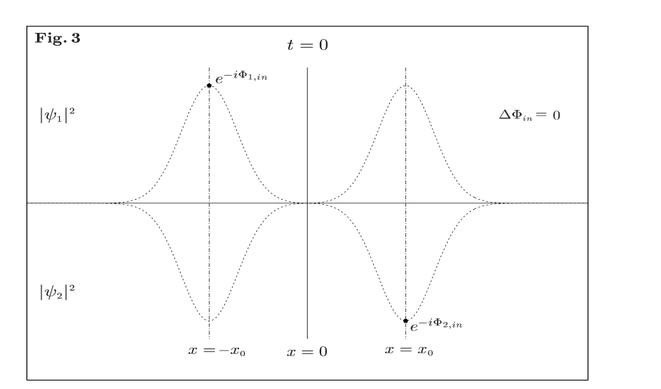
Figure 3: The square modulus of the mass eigenstate coefficients, $|\psi_{\mbox{\tiny$1$}}(x,t)|^{\mbox{\tiny$2$}}$ (upper-half) and $|\psi_{\mbox{\tiny$2$}}(x,t)|^{\mbox{\tiny$2$}}$ (lower-half), is plotted as a function of $x$ for the initial time $t=0$. As a model assumption, the wave packets are supposed to be generalized Gaussian functions peaked around $x=\pm x_{\mbox{\tiny$0$}}$.

To simplify the following calculation, we return to the unphysical (in any frame) $\Delta p=0$ scenario with instantaneous creation at $t=0$. We consider a wave packet obtained by a sum of generalized Gaussians with peaks at $x=\pm x_{\mbox{\tiny$0$}}$ (see Fig. 3),

$$\psi(x,0)=N\,\left\{\exp\left[i\,p_{\mbox{\tiny$0$}}(x+x_{\mbox{\tiny$0$}})\right]\,\exp\left[-\frac{\,\,(x+x_{\mbox{\tiny$0$}})^{\mbox{\tiny$2$}}}{\,\,a^{\mbox{\tiny$2$}}}\right]+\exp\left[i\,p_{\mbox{\tiny$0$}}(x-x_{\mbox{\tiny$0$}})\right]\,\exp\left[-\frac{\,\,(x-x_{\mbox{\tiny$0$}})^{\mbox{\tiny$2$}}}{\,\,a^{\mbox{\tiny$2$}}}\right]\right\}~{},$$ (28)

where $N$ is the normalization constant. We also assume that the peaks are well separated. In this case

$$N\approx\left(\frac{1}{\,2\pi a^{\mbox{\tiny$2$}}}\right)^{\mbox{\tiny$\frac{1}{4}$}}~{}.$$

Note that each gaussian has its own extra constant phase factor.

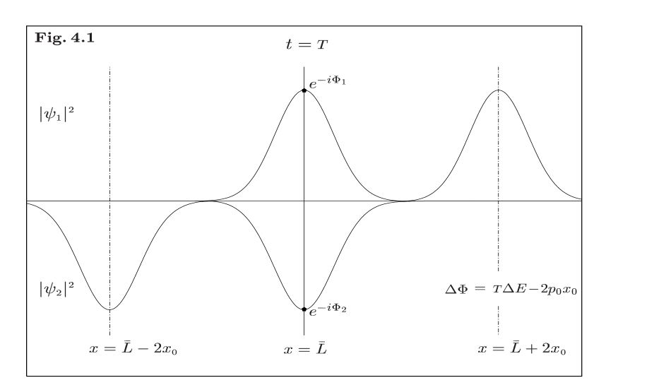
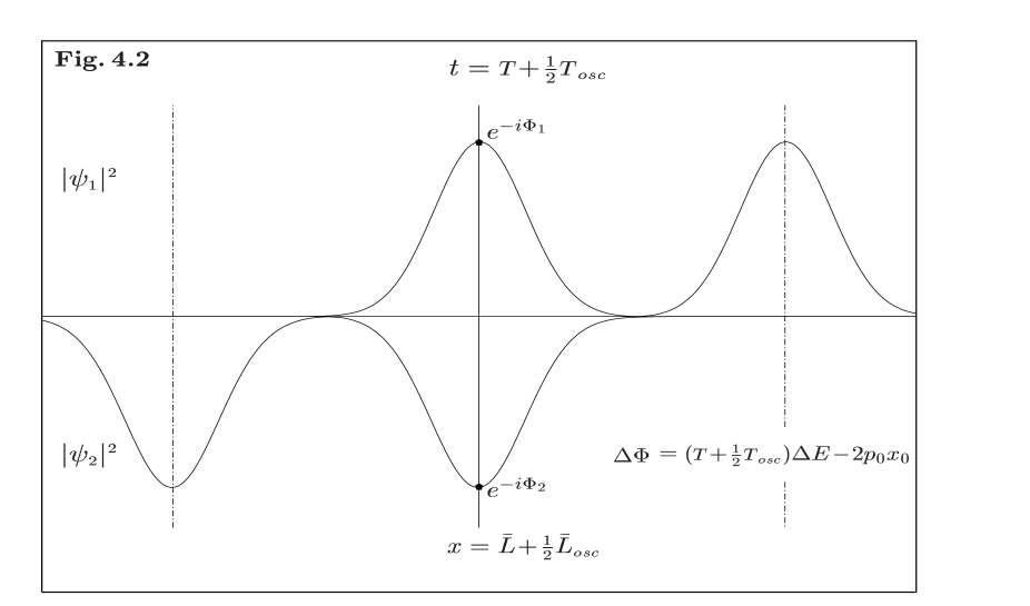
Figure 4: The square modulus of the mass eigenstate coefficients, $|\psi_{\mbox{\tiny$1$}}(x,t)|^{\mbox{\tiny$2$}}$ (upper-half) and $|\psi_{\mbox{\tiny$2$}}(x,t)|^{\mbox{\tiny$2$}}$ (lower-half), is plotted as a function of $x$ for two times: $t=T$ and $t=T+\frac{1}{2}\,T_{\mbox{\tiny$osc$}}$. The choice of $T=2x_{\mbox{\tiny$0$}}/\Delta v$ guarantees that the first peak (from the left) of the $\boldsymbol{\nu_{\mbox{\tiny$1$}}}$ mass eigenstate wave packet overlaps with the second peak of the $\boldsymbol{\nu_{\mbox{\tiny$2$}}}$ mass eigenstate wave packet. By observing that $T/T_{\mbox{\tiny$osc$}}\approx x_{\mbox{\tiny$0$}}\bar{E}\gg 1$ and using Eq. (29), it can be immediately understood why the plots of the mass eigenstate wave packets at the times $t=T$ and $t=T+\frac{1}{2}\,T_{\mbox{\tiny$osc$}}$ practically coincide.

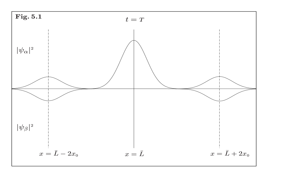
Figure 5: The square modulus of the flavor eigenstate coefficients, $|\psi_{\mbox{\tiny$\alpha$}}(x,t;\frac{\pi}{4})|^{\mbox{\tiny$2$}}$ (upper-half) and $|\psi_{\mbox{\tiny$\beta$}}(x,t;\frac{\pi}{4})|^{\mbox{\tiny$2$}}$ (lower-half), is plotted as a function of $x$ for two times: $t=T$ and $t=T+\frac{1}{2}\,T_{\mbox{\tiny$osc$}}$. The choice of $T=2x_{\mbox{\tiny$0$}}/\Delta v$ (which does not necessarily coincides with an integer number of standard oscillation period $T_{\mbox{\tiny$osc$}}$) corresponds to a (local) maximum probability to find the flavor state $\boldsymbol{\nu_{\mbox{\tiny$\alpha$}}}$ (upper plot). This would not agree with the prediction of the standard formula, because of the presence of the extra constant phase term. Nevertheless, the standard oscillation period is maintained. Indeed, at the later time $T+\frac{1}{2}\,T_{\mbox{\tiny$osc$}}$, we have a (local) maximum probability to find the flavor state $\boldsymbol{\nu_{\mbox{\tiny$\beta$}}}$ (lower plot).

We now allow the wave packets to evolve and consider the situation (measurement) in which the first peak of one mass eigenstate overlaps with the second peak of the other (see Fig. 4). In this region of overlap, oscillation occurs but it is to be noted that there are non-overlapping parts of the wave packet which correspond to pure mass eigenvalues (see Fig. 5). The contribution of these parts yields a non oscillating term. Indeed this is exactly what happens when the mass wave packets have completely separated (decoherence). The oscillating term is modified by the presence of the difference between the phase factors $\exp[ip_{\mbox{\tiny$0$}}x_{\mbox{\tiny$0$}}]$ and $\exp[-ip_{\mbox{\tiny$0$}}x_{\mbox{\tiny$0$}}]$. Thus, the oscillation formula at or around these times reads

$$P\left(\boldsymbol{\nu_{\mbox{\tiny$\alpha$}}}\to\boldsymbol{\nu_{\mbox{\tiny$\beta$}}};\,t\right)\approx\sin^{\mbox{\tiny$2$}}2\theta\left\{1-\mbox{$\frac{1}{2}$}\,\exp\left[-\,\left(\,\frac{\Delta v\,t-2x_{\mbox{\tiny$0$}}}{a\sqrt{2}}\right)^{\mbox{\tiny$2$}}\right]\,\cos\left[\left(\frac{\Delta m^{\mbox{\tiny$2$}}}{2\bar{E}}\,t\right)\mp 2p_{\mbox{\tiny$0$}}x_{\mbox{\tiny$0$}}\right]\right\}\,/\,2~{},$$ (29)

where the sign in the constant term $\mp\,2p_{\mbox{\tiny$0$}}x_{\mbox{\tiny$0$}}$ depends on $v_{\mbox{\tiny$1$}}\mbox{\footnotesize$\gtrless$}\,v_{\mbox{\tiny$2$}}$. In this picture,

$$2p_{\mbox{\tiny$0$}}x_{\mbox{\tiny$0$}}\approx\pm\,p_{\mbox{\tiny$0$}}\Delta v\,t\approx\mp\,\frac{\Delta m^{\mbox{\tiny$2$}}}{2\bar{E}}\,t~{}.$$

Thus, we obtain the extra factor two of Section II for the oscillating phase. It is true that since $\mp\,2p_{\mbox{\tiny$0$}}x_{\mbox{\tiny$0$}}$ is a constant term the oscillation period is still be the standard one (see Fig. 5). However, with multiple peaks, each with independent initial constant phases, the effective extra phase term could become $L$ or $T$ dependent. We see no good physical reasons for excluding such a contribution a priori.

In the case of minimal slippage when the interference occurs within each separate peak, the constant phases play no role. In these cases, we can also ignore (by definition) the non-overlapping parts of the wave function. Thus, the standard result is obtained as a good approximation. This is now consistent with the fact that for no slippage ($\Delta v=0$) the standard formula is exact.

It is also useful to observe that, in the incoherent limit, one has a clean method for determining experimentally the mixing angle, whatever the wave packet form is,

$$P\left(\boldsymbol{\nu_{\mbox{\tiny$\alpha$}}}\to\boldsymbol{\nu_{\mbox{\tiny$\beta$}}};\,T\gg a/|\Delta v|\right)=\sin^{\mbox{\tiny$2$}}2\theta\,/\,2~{}.$$

Nevertheless, the time for the onset of complete incoherence depends upon the wave packet dimensions and upon the different mass velocities.

VII. CONCLUSIONS

The aim of this work was to shed some new light on the quantum mechanics of particle oscillations. The primary objective was to search for the conditions under which the standard oscillation formula is valid. In the process we have understood the origin of the extra factors in the plane wave oscillation calculations. It is the implicit assumption that at creation (whether instantaneous or not) the flavor eigenstate is unique even up to the phase at all points and times of creation. To the best of our knowledge this has not been pointed out previously. The often quoted plane wave derivations of the standard formula have generally been based upon invalid approximations or formalisms chosen so as to compensate for the neglect of the initial phase contributions.

Other authors have previously pointed out that the assumptions of equal velocity, momentum and energy are “unphysical” in the sense that they are not compatible with the known production processes in the laboratory frame. We have pointed out here that the first two are rigourously non physical in the sense that there is no Lorentz frame in which they occur. Only the equal energy case is theoretically possible. Consequently, since the assumption of instantaneous creation together with flavor eigenstate production imposes equal momentum, it is non physical. We can correct for this by assuming an event-wise production mechanism. Event-wise production is perfectly natural. It is even predicted for the equal momentum case (had it existed) when seen by another observer in a Lorentz frame in which the momenta are not equal. Somewhat surprisingly the standard oscillation phase, as calculated in the wave packet formalism, is not affected by this modification, at least not for the cases with minimal slippage. Thus, we have concluded that within the wave packet formalism the standard result is not only exact in the case of equal velocities (no slippage) but also a good approximation in all cases in which minimal slippage occurs between the mass wave packets.

Now the standard oscillation formula contains no dependence upon the form of the wave packets involved. This clearly cannot be valid in general. Indeed, as a simple and well known counter example we have recalled in the previous Section the incoherence limit, who’s onset is dependent upon the size of the wave packets and the differences in the mass eigenstate velocities. One must expect the dimensions and explicit form of the wave packets, including all relative phases, to play a role in the oscillation formula. We have exhibited a simple two-gaussian model to demonstrate not only this but also how a result that simulates the extra-factors calculations (for the oscillating part) can be obtained.

Allowing for completely arbitrary modulations of the plane waves, we must introduce additional parameters into our generalized formula

$$P\left(\boldsymbol{\nu_{\mbox{\tiny$\alpha$}}}\to\boldsymbol{\nu_{\mbox{\tiny$\beta$}}};\,t\right)=\sin^{\mbox{\tiny$2$}}2\theta\left\{1-R(t)\,\cos\left[\frac{\Delta m^{\mbox{\tiny$2$}}}{2\bar{E}}\,t+\varphi(t)\right]\right\}\,/\,2~{},$$ (30)

where $R(t)$ and $\varphi(t)$ depend upon the details of the wave packet envelope. This formula contains two extra parameters when compared to the standard formula, four in all. It may well prove necessary to employ our generalized expression in order to reconcile diverse experimental results. The alternative could lead to inconsistencies in the determination of mass differences and/or mixing angles. Use of this formula may also avoid the need to introduce one or more sterile neutrinos. This equation, as it stands, is probably too vague for practical phenomenological fits. However, it is always possible, without returning to the standard formula, to add simplifying assumptions such as the time independence of the extra phase term.

Apart from the question posed in this paper of what is the most practical oscillation formula to be used in phenomenological fits, there is an aspect of this work which is of great interest, at least to the authors. The details of the creation and annihilation of wave packets is to a large degree unknown territory. Oscillation phenomena may indeed be useful as a source of information upon this subject. It should also be possible to investigate this aspect for photon wave packets with the help of very precise measurements in interference phenomena. In the case of photons the effect of slippage is substituted by the occurrence of different path lengths. For example, in optics it is well known that interference effects cease if the difference of path lengths exceeds the wave packet dimension, and this should permit the determination of these dimensions. This technique may, of course, also be extended to any elementary particle that lives long enough. This particular subject matter recalls transitory phenomena in various sectors of classical physics. Its study, both theoretical and experimental, at the quantum mechanical level is surely a great challenge.

Figure 1: The square modulus of the mass eigenstate coefficients, $|\psi_{\mbox{\tiny$1$}}(x,t)|^{\mbox{\tiny$2$}}$ (upper-half) and $|\psi_{\mbox{\tiny$2$}}(x,t)|^{\mbox{\tiny$2$}}$ (lower-half), is plotted as a fucntion of $x$ for two times: $t=0$ (left-side) and $t=T$ (right-side). As a model assumption, the wave packets are supposed to be Gaussian functions (with the same width $a$) peaked around $x=0$. At observation time $T$, the mass eigenstate wave packets are centered around different space-points, $L_{\mbox{\tiny$1$}}=v_{\mbox{\tiny$1$}}T$ and $L_{\mbox{\tiny$2$}}=v_{\mbox{\tiny$2$}}T$ (spreading effects are neglected). Since $L_{\mbox{\tiny$1$}}$ and $L_{\mbox{\tiny$2$}}$ are assumed very large compared to $a$, the plots of the mass eigenstate wave packets at creation and observation are separated by dots in the $x$-axis. At observation time $T$, $x_{\mbox{\tiny$f$}}$ is a fixed point in the overllaping region. At this point, the mass eigenstate phases are given by $\Phi_{\mbox{\tiny$1$}}(x_{\mbox{\tiny$f$}},T)=E_{\mbox{\tiny$1$}}T-p_{\mbox{\tiny$1$}}v_{\mbox{\tiny$1$}}T$ and $\Phi_{\mbox{\tiny$2$}}(x_{\mbox{\tiny$f$}},T)=E_{\mbox{\tiny$2$}}T-p_{\mbox{\tiny$2$}}v_{\mbox{\tiny$2$}}T$. The interfering wave packet points at $(x_{\mbox{\tiny$f$}},T)$ correspond to different initial wave packet points. Thus, the initial phases $\Phi_{\mbox{\tiny$1$},\mbox{\tiny$in$}}(x_{\mbox{\tiny$f$}}-v_{\mbox{\tiny$1$}}T,0)=-p_{\mbox{\tiny$1$}}x_{\mbox{\tiny$f$}}+p_{\mbox{\tiny$1$}}v_{\mbox{\tiny$1$}}T$ and $\Phi_{\mbox{\tiny$2$},\mbox{\tiny$in$}}(x_{\mbox{\tiny$f$}}-v_{\mbox{\tiny$2$}}T,0)=-p_{\mbox{\tiny$2$}}x_{\mbox{\tiny$f$}}+p_{\mbox{\tiny$2$}}v_{\mbox{\tiny$2$}}T$ are automatically included in the wave packet formalism. Consequently, the standard result $T\Delta E-x_{\mbox{\tiny$f$}}\Delta p$ is obtained.

Figure 2: The square modulus of the flavor eigenstate coefficients, $|\psi_{\mbox{\tiny$\alpha$}}(x,t;\frac{\pi}{4})|^{\mbox{\tiny$2$}}$ (upper-half) and $|\psi_{\mbox{\tiny$\beta$}}(x,t;\frac{\pi}{4})|^{\mbox{\tiny$2$}}$ (lower-half), is plotted as a function of $x$ for two times: $t=0$ (left-side) and $t=T$ (right-side). The observation time $T$ was chosen as an integer number of standard oscillation periods, $T_{\mbox{\tiny$osc$}}=4\pi\bar{E}/\Delta m^{\mbox{\tiny$2$}}$. In the case $\Delta p=0$, a pure falvor state $\boldsymbol{\nu_{\mbox{\tiny$\alpha$}}}$ is created at time $t=0$ (upper plot). Slippage (see Fig. 1) leads to a non zero probability to find a flavor state $\boldsymbol{\nu_{\mbox{\tiny$\beta$}}}$ at time $T$. However, in the case $\Delta p\neq 0$, within the context of instantaneous creation, there does not exist any time for which the state is a pure flavor eigenstate (lower plot)

.

References

• [1] M. Zralek, Acta Phys, Polon. B 29, 3925 (1998).
• [2] K. Zuber, Phys. Rept. 305, 295 (1998).
• [3] S. Bilenky, C. Giunti, and W. Grimus, Prog. Part. Nucl. Phys. 43, 1 (1999).
• [4] H. J. Lipkin, Phys. Lett. B 348, 604 (1995).
• [5] Y. Grossman and H. J. Lipkin, Phys. Rev. D 55, 2760 (1997).
• [6] Y. Takeuchi, Y. Tazaki, S. Tsai, and T. Yamazaki, Mod. Phys. Lett. A 14, 2329 (1999).
• [7] L. B. Okun and I. S. Tsukerman, Mod. Phys. Lett. A 15, 1481 (2000).
• [8] S. De Leo, G. Ducati, and P. Rotelli, Mod. Phys. Lett. A 15, 2057 (2000).
• [9] Y. Takeuchi, Y. Tazaki, S. Tsai, and T. Yamazaki, Prog. Theor. Phys. 105, 471 (2001).
• [10] J. H. Field, The description of neutrino and muon oscillations by interfering amplitudes of classical space-time paths (hep-ph/0110064).
• [11] C. Giunti, The phase of neutrino oscillations (hep-ph/0202063).
• [12] P. Rotelli, “Invalid approximations in the oscillation formula” in NOW 2000, Proceedings of the Europhysics Neutrino Oscillation Workshop (Ed. G. Fogli, North-Holland 2001).
• [13] B. Kayser, Eur. J. Phys. C 15, 344 (2000).
• [14] C. Giunti, and C. W. Kim, Phys. Rev. D 58, 017301 (1998).
• [15] S. M. Bilenky and B. Pontecorvo, Phys. Rept. 41, 225 (1978).
• [16] S. M. Bilenky and S. T. Petcov, Rev. Mod. Phys. 59, 671 (1987).
• [17] B. Kayser, F. Gibrat-Debu, and F. Perrier, The Physics of Massive Neutrinos (World Scientific, Singapore, 1989).
• [18] F. Bohem and P. Vogel, Physics of Massive Neutrinos, (Cambridge University Press, Cambridge, 1992).
• [19] C. W. Kim and A. Pevsner, Neutrinos in Physics and Astrophysics, (Harwood Academic Publishers, Langhorne, 1993).
• [20] V. Gribov and B. Pontecorvo, Phys. Lett. B 28, 493 (1969).
• [21] H. Fritsch and P. Minkowsky, Phys. Lett. B 62, 72 (1976).
• [22] J. Lowe, B. Bassaleck, H. Burkhardt, A. Rusek, G. J. Stephenson Jr, and T. Goldman, Phys. Lett. B 384, 288 (1996).
• [23] K. Kiers and N. Weiss, Phys. Rev. D 57, 3091 (1998).
• [24] B. Kayser, Phys. Rev. D 24, 110 (1981).
• [25] J. Rich, Phys. Rev. D 48, 4318 (1993).
• [26] R. G. Winter, Lett. Nuovo Cimento 30, 101 (1981).
• [27] C. Giunti, Mod. Phys. Lett. A 16, 2636 (2001).
Refer to caption