Resummed event-shape variables in DIS.
Abstract:
We complete our study of resummed event-shape distributions in DIS by presenting results for the class of observables that includes the current jet mass, the -parameter and the thrust with respect to the current-hemisphere thrust axis. We then compare our results to data for all observables for which data exist, fitting for and testing the universality of non-perturbative effects. A number of technical issues arise, including the extension of the concept of non-globalness to the case of discontinuous globalness; singularities and non-convergence of distributions other than in the Born limit; methods to speed up fixed-order Monte Carlo programs by up to an order of magnitude, relevant when dealing with many and points; and the estimation of uncertainties on the predictions.
LPTHE–02–040
hep-ph/0208073
August 2002
1 Introduction
Quantum chromodynamics is special among the theories of the standard model in that its strongly and moderately coupled domains are within reach of experiment, and indeed unavoidable at current energies. This leads to a wealth of non-trivial phenomena involving multiple particle production, divergent perturbative series and large non-perturbative effects even at formally perturbative scales. A full understanding of such phenomena remains one of the main aims of QCD, both because of their fundamental interest and because they are inextricably present in any measurement involving hadrons, be it a determination of the properties of QCD itself or even searches for new physics.
A feature of QCD is that the more exclusive an observable, the more difficult it is to predict. This is because more exclusive observables often involve several disparate scales, and higher-order terms in the perturbative series have coefficients which are enhanced by (large) logarithms of ratios of scales. Furthermore whenever the observable involves integrals over phase space which extend significantly into the infrared, or when one of the scales is close to the strong-coupling region, the observable is likely to be subject to large non-perturbative contributions.
A class of observables involving an interesting compromise between infrared sensitivity and perturbative calculability is that of event shapes and their distributions. These infrared-collinear (IRC) safe observables measure properties of the flow of energy-momentum, for example the normalised squared invariant mass of a hemisphere, . When pushing such observables to the exclusive limit (in the case of , small invariant masses) the perturbative distribution develops double logarithms at each order of perturbation theory , which must be resummed to all orders. Furthermore because such observables are usually linear in soft momenta, there are significant non-perturbative effects, formally of order , which cannot be ignored.
This class of observables has already been widely examined for -jet events in collisions and resummations of large-logarithmic terms [1, 2, 3, 4, 5, 6] have been in existence for some time now. The literature is at first sight slightly confusing when it comes to defining the accuracy of these resummations. Let us use to denote the probability that the jet mass is smaller than some value . Then we can write as
| (1) |
One can define leading logarithms (LL) as consisting of all terms with , next-to-leading logarithms (NLL) as terms with , and so on (e.g. [3, 7]). In this terminology, the state of the art for resummations is NNLL order, and in terms of relative accuracies on it means that for , is determined to within relative corrections of order .
For however, any fixed order of logarithmic resummation in this hierarchy, NpLL, loses its predictive power, because there will always be neglected terms , with , which are formally larger than . Fortunately many observables can be shown to exponentiate, which means that we are entitled to write
| (2) |
(in some cases needs to be broken up into a sum of terms, each of which exponentiates, but with different exponents). With this form of expansion, leading logarithms now refer to all terms , while next-to-leading logs (or single logs — SL) are those with (e.g. [1]). The state of the art in this form of expansion is NLL accuracy. It means that for the neglected terms correspond to modifications of of relative order . More generally, for observables that do not exponentiate, one can use this condition on the relative size of higher-order corrections to define NLL accuracy.
There is partial overlap between the terms needed for NNLL accuracy in and NLL accuracy in . Our aim is to guarantee both, though unless we explicitly specify otherwise, our statements of accuracy will refer to the expansion of .
With the 2-jet NLL calculations, there have been extensive comparisons to data (see for example [8]) and much has been learnt from these studies, especially regarding our understanding of hadronisation effects, for which several related theoretical approaches (e.g. [9, 10, 11, 12, 13, 14, 15, 16]), mostly based on renormalons [17], have been developed and tested.
Of course, event-shape observables are not restricted to collisions and there are good reasons to extend their study to other processes. Many of the hadronisation models embody a concept of universality, whereby all hadronisation effects should be governed by a restricted set of non-perturbative parameters which are both observable and process independent. In event-shapes there is good evidence in favour of universality [18], but in order to be fully established it needs to be tested in processes involving incoming hadrons as well. It is also important that the perturbative predictions for exclusive final-state properties be tested in a wider context than just , both so as to establish confidence in their general applicability and in view of the fact that they may well come to play a role in searches for new physics through studies of the radiation pattern associated with the different colour flows that are relevant in ‘new physics’ processes as opposed to the QCD backgrounds [19].
It was to investigate these issues in more detail that a study of NLL resummed DIS Breit-frame current-hemisphere () event-shape observables was initiated in [20, 21, 22]. From the point of view of studying hadronisation effects, DIS observables are particularly interesting in that there is a considerable amount of data [23, 24, 25] over a wide range of values (within the same experiment), making it possible to explicitly test the predicted -dependence of hadronisation effects. This was part of the motivation for the original theoretical studies [26, 27] of hadronisation effects in mean values of DIS event shapes.
The DIS resummations carried out in [20, 22] dealt with observables defined with respect to the boson () axis — two variants of the thrust ( and ) and one of the jet broadening (). In the current paper we complete our study of resummed DIS event-shapes by presenting results for three observables defined independently of the boson axis (except through the restriction that only particles in are measured) and by comparing all of our resummed results to data.111Except for for which no data currently exist.
The three observables resummed in this paper are the thrust with respect to the thrust axis and normalised to the current hemisphere energy, , the invariant squared jet mass, and the -parameter, . Their exact definitions are as follows:
| (3) |
| (4) |
| (5) |
Additionally, we refer to . Events where the energy in the current hemisphere is less than some value are discarded. This is necessary to ensure the all-order infrared and collinear (IRC) safety of the observable, in particular to protect against divergences associated with events containing hard emissions in the remnant hemisphere () alone and arbitrarily soft emissions in . It is important that not be too small a fraction of the photon virtuality , in order to avoid developing large terms.
The fact that the above observables do not involve the boson axis in their definitions means that they are essentially insensitive to radiation in the remnant hemisphere — this is in contrast to the boson axis observables considered previously, which were all sensitive to radiation in through recoil effects on the current quark. This has several consequences for the resummation: the double-logs are less strong because they only involve the suppression of soft and collinear radiation from one hard parton; a fraction of the time, the hard parton in is not a quark but a gluon, implying different colour factors for the double-logs; at the single log-level the appropriate factorisation scale for the parton distributions is , independently of the value of the observable; and the resummation has non-global single-logs, discovered recently in [28, 29] which involve multiple energy-ordered large-angle gluons in emitting coherently into .
The different aspects of the resummation are discussed in sections 2, 3 and 4 with the latter section addressing also the issue of previously neglected non-global logarithms for the boson-axis observables. This leads to our introducing the concept of discontinuously global variables such as and dynamically discontinuously-global variables such as . In practice the phenomenological impact of the non-global logarithms on these observables is small.
In addition to there being a need for a resummation in the single current-jet limit (), it turns out that there are poorly convergent, log-enhanced structures in other regions of phase space, associated with discontinuities or non-smoothness in low-order distributions. These are analogous to the problems seen for the -parameter at , and a resummation generally leads to a smoothing-out of these structures [30]. In most cases their impact is restricted to a relatively small region, so in section 5 we limit ourselves to illustrating the origin of the problems for the the DIS parameter, and giving a list of the non-smooth structures that arise for the other observables. We do not carry out any resummation of these observables around the singular structures, restricting ourselves to resummation near the exclusive boundary, , where is the event shape in question.
Another, technical, issue that needs to be dealt with is that of determining the fixed-order distributions for all the observables. This turns out to be a very computer-intensive process if one wishes to obtain a reasonable precision and resolution. So in section 6 we present a method for speeding up fixed-order Monte Carlo programs such as disent[31] or disaster++ [32] through the reuse of the same event to calculate many and points at the same time.
Once one has the resummed and fixed-order predictions (matched with the procedures of [1, 22]) one can then address (section 7) the issue of including non-perturbative corrections. We follow the approach of [11, 12, 33] based on the concept of a universal infrared-finite coupling, where the power correction is essentially a shift of the distribution by an amount which depends on a moment of the coupling in the infrared and on a calculable, observable-dependent coefficient (as determined in [26, 27, 22]).
With all the ingredients in place we then show, in section 8 the impact of the resummation, and discuss choices and uncertainties associated with unknown higher-orders and with certain prescriptions for the non-perturbative effects.
2 Kinematics
Here we establish the kinematic properties of the different variables in which we are interested. The expressions derived will be approximate but sufficient for single-log/next-to-leading log (NLL) accuracy.
In order to achieve this precision we need to consider configurations of soft and/or collinear gluons in addition to the hard initiating parton (quark or gluon). To be precise we want expressions for the observable in several kinematic configurations:
-
•
A hard particle in , close to the boson axis, accompanied by any number of soft and collinear gluons. Here the expression for the observable has to be correct to within terms of relative order of a power of the softness so as to account for both double and single logs.
-
•
A hard particle (close to the boson axis) in along with an energetic almost collinear gluon. This region is only associated with single-logs and the expression for the observable need simply be correct to within an overall factor (because replacing by , with some fixed number, is equivalent to a NNLL change).
-
•
A hard particle (close to the boson axis) in accompanied by a soft wide-angle gluon in . This situation is also responsible only for single logs and so it is again sufficient to have an expression for the observable correct to within an overall factor.
-
•
A hard particle in away from the boson axis, accompanied by any number of particles soft and collinear to the hard parton. This kind of hard configuration is suppressed by a power of and so only gives NNLL terms (both in and in ). There it is sufficient to have an expression for the observable valid to within an overall factor.
In addition, for our resummation approach to be valid, the conditions for exponentiation (discussed in [22, 6]) must also hold. This is the case for all the observables discussed here.
What we shall actually do is derive expressions for the jet mass, which has already been considered in various related cases in [34, 35, 28], and then show that to the accuracy that we need, other observables are related to it by a constant factor.
We first obtain an expression for relevant for many soft (and optionally collinear) emissions. We take a hard parton , close to the photon axis and with energy , and any number of soft and collinear particles , with energies and angles to the hard parton. We denote by the total energy of all particles in .
With this kinematics, the jet mass is given by
| (6) |
To extend this result to the case of a single hard collinear emission, , we need to take into account the recoil of the hard parton and the result for is
| (7) |
This is the information used for example in the resummations of [34, 35, 28].
An expression for the thrust in terms of the jet mass, in the limit where all emissions are soft (and at a polar angle of less than from the quark direction) and/or collinear, can be obtained by noting that in this limit the thrust axis coincides with the direction given by the sum of all three-momenta in the hemisphere, as in the case [1].
Denoting by the total vector -momentum sum, we can rewrite as
| (8) |
while the thrust is given by
| (9) |
where we have made use of the condition that none of the particles is moving backwards with respect to .
In the limit , implying , we immediately see that , allowing us to reuse the resummation for , simply replacing every occurrence of with .222Strictly speaking, for this to be true one also needs the easily demonstrated property that when the hard particle is at large angles (and emitted gluons can move backwards with respect to the thrust axis and still be in ).
In the case of the -parameter we need to explicitly derive expressions for it before being able to compare to the jet mass. Starting from eq. (5) we see that for any number of soft (and optionally collinear) emissions:
| (10) |
while for a single hard collinear emission, , we have to take into account the recoil of the hard parton to get
| (11) |
Comparing to the corresponding expressions for the jet-mass we see that in the presence of collinear emissions (many soft or one hard) . For large-angle soft emissions we do not have an exact proportionality, but both and receive contributions proportional to and so should have the same large-angle single logs. Therefore the resummed result for is simply that for with the replacement .
One final point to note is that because and are proportional in all situations involving a single soft or collinear emission in , the corresponding pure contributions to the resummed results (the terms discussed below) are identical, and the coefficients of the power corrections are also related by the same proportionality factor. In contrast, because of the different dependence on large-angle soft emissions, for one of the constant terms differs (by a -function in ), as discussed in appendix B and the power correction is not times larger than that for , but rather only times larger.
3 Resummation
To write down a resummed result to NLL accuracy for the current hemisphere jet mass we simply refer to Ref. [28]. There we established a formula for the hemisphere jet mass in annihilation and an essentially identical form applies here. We define the integrated current hemisphere jet mass distribution at a given ,
| (12) |
where is the Born cross section.333We could equally well have normalised to the total cross section, but this would lead to the order perturbative expansion for involving combinations of parton distributions such as . It is thus simpler to calculate defined as normalised to the Born cross section and then to renormalise it as appropriate when comparing to data. This integrated jet-mass distribution is given to NLL accuracy by the expression
| (13) |
The precise analytical forms for the different elements in this equation are given in the appendices. Here we limit ourselves to an explanation of the physical meaning of the various factors.
The first term in eq. (13) accounts for situations in which the hard particle in is a quark; is the form factor for the hemisphere mass to be less than assuming just independent eikonal emission off a line (including hard collinear corrections). It can be written as
| (14) |
in terms of the jet-mass distribution, , computed several years ago [34, 35]. It contains both double and single logarithms.
The factor embodies the single-logarithmic corrections associated with the fact that is non-global, namely that it measures emissions in only. This means that a constraint on does not imply any explicit constraint on emissions in , and large-angle gluons in are actually radiated off an ensemble of energy-ordered large-angle gluons in . Thus the pattern of large-angle gluon radiation in differs from independent emission off an eikonal line at the single logarithmic level, and this needs to be accounted for with the factor , as discussed in more detail in section 4 (together with related, but rather subtle contributions that were neglected in our previous work [20, 22]). It is to be noted that beyond order , is known only numerically and in the large- limit.
The -independent contribution is the only piece in the first term of (13) that is sensitive to the parton distribution functions (PDFs). It has a number of separate, though not always separately well-defined, origins. One physically identifiable contribution to is from the configuration where one has a lone hard quark in and a gluon in . This on its own is divergent and cancels against corresponding virtual corrections and against the term from the factorisation of the parton distribution functions (PDFs). This implies that has both factorisation scheme and scale dependence, similar to what is discussed in appendix A of [20] (Eqs. (A.9) and (A.10)). It should be kept in mind that when there is a hard large-angle gluon in , then the hard quark in will not be aligned along the boson axis nor will it have energy , and a number of the approximations made at single log level in and will be incorrect — however this is beyond our accuracy, because it is relevant only a fraction of the time.
The remainder of is associated with approximations made in for the pattern of real and virtual corrections for a hard gluons and (in some cases) with approximations for the dependence of the observable on soft large-angle and hard collinear emissions. We note that configurations with an empty (strictly ) are considered as having an undefined value of the jet mass, and so are not included in the integral for and correspondingly in the definition of .
A final point to note about the piece is that when considering , as we usually do, and defining our hierarchy in terms of the series expansion of , the terms are not formally needed to NLL accuracy. In contrast if we are in the region and looking at the expansion of to NNLL accuracy, then the terms are needed.
Let us now come to the second term of eq. (13). This accounts for the situation in which the hard parton in is a gluon. This happens in only a fraction of events, and the form factor (also given in [34, 35]) is related at leading-log level to by replacing with in the exponent. At single log level in the situation would be more complicated because we cannot make the approximation of the gluon being aligned along the boson axis or of its having energy . However as in the case of , given that this whole term is multiplied by , to our overall level of accuracy we are free to mistreat single-logs in . In practice we systematically neglect all single-log contributions in this term, including those from non-global effects (which could have been represented by an extra factor in (13)).
Finally we recall that in order to derive a result for the and distributions one just replaces by and respectively throughout eq. (13) — the , and functions have identical forms for all the above variables. It should however be noted that while the coefficient function is the same for the and variables, it is different for the parameter (see appendix B).
4 Non-global logarithms and discontinuously global observables
In a previous paper we introduced the concept of a non-global observable, defined as an observable sensitive to emissions only in a restricted angular portion of phase space. We pointed out that at single-logarithmic accuracy, such observables receive a set of contributions associated with energy-ordered large-angle emissions, termed non-global logarithms [28]. In this section, we wish to refine that definition.
4.1 Non-global logs
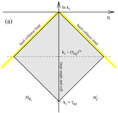
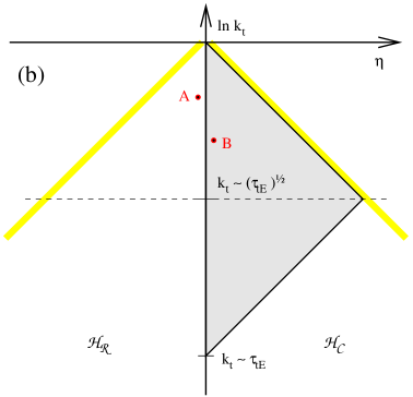
The difference between a global observable and a non-global one is illustrated in fig. 1, which shows in grey the phase-space regions where emissions are forbidden if the observable’s value is to be below a given value . In the left hand figure we consider the global observable , whose value for a given ensemble of emissions is
| (15) |
where the sum runs over all soft (and collinear) particles and the transverse momenta are implicitly normalised to for brevity. For observables like it is safe to neglect energy-ordered large-angle contributions as can be seen by considering the case with two emissions and , with and : the modification of the observable’s value by emission is negligible, , and there will be full cancellation (at the single-log level) between real and virtual contributions for .
A non-global observable is one such as , illustrated in fig. 1b. The observable’s value is given by (cf. eq. (9))
| (16) |
i.e. there is only sensitivity to emissions in the current hemisphere, and placing a constraint on the value of the observable implies no direct constraint on emissions in .444In writing the above formula for we have neglected configurations in which there is a hard parton (quark or gluon) at a large angle to the the boson axis. This is because the overall contribution from non-global logs in such situations is (including the configuration probability ) and hence subleading.
In fig. 1b, this translates to only the current-hemisphere region being shaded. Now let us consider the situation with emissions and as shown in the figure, and both emissions at large angles, with in and in . Emission does not contribute to the observable. Emission would contribute, since it is in the shaded region — so it must be forbidden, corresponding to a resummation of virtual corrections. However the form factor in eqs. (13) and (14) is derived with the assumption that the pattern of soft large-angle emission is that off an eikonal current, whereas the presence of at large angles in modifies the pattern of large-angle soft emissions in (and the corresponding virtual corrections) to be that from a antenna.
So it is necessary to correct for the fact that the emission pattern is not that from a pair, but in general that from an ensemble that can contain any number of energy-ordered large-angle gluons in . At the two gluon level shown in fig. 1b the correction to is of the form
| (17) |
where the double integration over transverse momentum is associated with the relevant ranges of and .
4.2 Discontinuously global observables
While the definition given above for a non-global observable is sufficient to ensure the presence of non-global logarithms, the converse is not true: it turns out that there exist observables that are global, but which are nonetheless subject to non-global logarithms.
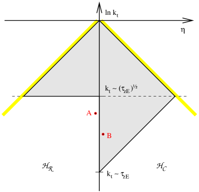
An example is whose value is
| (19) |
The region of phase space to be excluded for the observable to have smaller than some given small threshold is shown in fig. 2. The whole angular extent of phase space is relevant, so the observable is global. However the dependence of the observable on emissions in and is parametrically different, going as and respectively. To denote this kind of observable, we introduce a new term: a discontinuously global observable. This is defined as being an observable, which, while sensitive to emissions in the whole angular reach of phase space, has a parametric dependence on (or energy) which changes discontinuously across one or more boundaries in angle.555Strictly speaking the parametric dependence may actually change smoothly, as long as the regions of different parametric dependence are separated by a limited region in angle.
In the case of , non-global logarithms arise through emission patterns of the kind represented by gluons A and B in fig. 2. Large-angle emission of into will not contribute significantly to the observable as long as . However it will modify the pattern of large-angle emissions B in when . On the other hand large-angle emission B in must be forbidden if . Therefore there is an energy-ordered region in which we should account for the modification of the emission pattern of by the presence of . This gives a non-global log, which at second order in contributes as
| (20) |
i.e. one quarter of the contribution in the fully non-global case, eq. (17). Analogously, at all orders we will have the same function as for the non-global , but with a different integration range in the definition of :
| (21) |
This non-global contribution was erroneously omitted in the original resummation for [20]. This ought, in principle, to have been revealed by the comparison with fixed-order calculations, however in practice the numerical accuracy of the fixed-order calculations is such that it is not possible to distinguish between comparisons with and without the non-global logs (this is specific to — other observables such as have effects which are four times larger and which therefore can be more straightforwardly distinguished in comparisons to fixed-order calculations).
4.3 Dynamically discontinuously global observables
An even more subtle situation involving non-global logarithms is that of the rather clumsily named ‘dynamically discontinuously global observables.’ These are observables which in a two-emission analysis (such as figs. 1, 2) appear to be global without discontinuities, but which develop a discontinuity dynamically at all orders. To illustrate what we mean, we consider the broadening with respect to the photon axis, . This is given by
| (22) |
Note that the parametric dependence on is the same in both hemispheres (there is a change in normalisation dependence in going from one hemisphere to another, but this is not sufficient to induce single-logarithms).
There is a subtlety however in that it is possible for to be parametrically smaller than some of the individual ’s in , if there is a cancellation in the vector sum. So for emissions in it is in principle possible to have and one is then faced with the issue that such emissions, when they are at large angles, modify the pattern of emissions into . At first sight this may seem quite unlikely because of the small probability of a sufficient cancellation in the vector sum. However as discussed in [22], at sufficiently small values of the broadening the favoured mechanism for obtaining a small value of is the cancellation in the vector sum, rather than the suppression of emissions. In such a situation non-global logarithms will arise.
In [22] we addressed the issue of this vector cancellation in some detail, showing that it was associated with a divergence in the pure NLL resummation and discussing how to improve the resummation to maintain the accuracy of there being only relative corrections in the region. However that treatment is incomplete since it did not take into account the non-global logarithms that arise in this context due to the dynamically discontinuous globalness.
From a phenomenological point of view, it is perhaps fortunate that these issues become relevant only considerably to the left of the Sudakov peak, a region that we ignore in the comparisons to data shown later. Indeed in the fits to data we use the pure NLL resummed formula for the broadening, for which there are no non-global logarithms.
4.4 Phenomenological impact of non-global logs
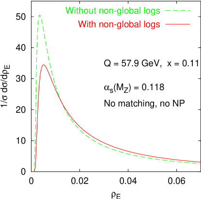
In figure 3 we illustrate the effect of non-global logarithms in the resummation of (other non-global observables are similar). The figure compares (unmatched) resummations with and without account of non-global logs. One sees that neglecting them leads to an overestimate of the peak-height by almost , though elsewhere in the distribution, the effect is smaller. In practice, matching to fixed-order calculations reduces the impact of neglecting the non-global logarithms, but the effects are still of the order of to .
The effect of non-global logs in the discontinuously global observable (not shown), is found to be smaller, at about the level. This is consistent with the naive expectation (cf. section 4.2) of a reduction by a factor of four compared to the non-global case. In section 9 we examine the effect of the non-global logarithms in fits for and the non-perturbative parameter.
5 Singularities other than at
The main aim of this paper is to discuss the resummation of the singular behaviour of distributions around . However, as was pointed out in [30] there can also be singular behaviour inside the phase space of certain observables, the notable example in scattering being the -parameter. In DIS the problem turns out to be much more common than in , even involving (in some cases) two divergent structures inside the phase space of a single observable. This is in part because one only counts particles in and hence there is a sharp angular cut-off (the interface of and ) which can introduce problems of non-smoothness in the various event shapes.
Divergences inside the phase space are associated with discontinuous or non-smooth structures at some lower order of perturbation theory. Higher order corrections act to smooth out these features, but order by order are divergent. One example of this is that in the LO distribution for the -parameter has a step function at ; the inclusion of all higher orders smooths out the step to give a ‘Sudakov shoulder,’ [30], though order by order the shoulder is associated with (a divergent series of singular) terms.
Such resummations, while interesting, are beyond the scope of this article. One should nevertheless be aware of the kinds of non-smoothness that arise in the different observables. We shall discuss in particular the DIS -parameter, and then give a summary of the properties of other observables.
5.1 The -parameter
It is convenient here to use the variables and defined in [26], such that the incoming quark, outgoing quark and outgoing gluon have respectively (Breit-frame) momenta , and , where
| (23a) | ||||
| (23b) | ||||
| (23c) | ||||
with
| (24) | |||||


The left-hand part of fig. 4 shows the different regions in the plane:
| A: and | B: | |
|---|---|---|
| C: | D: empty |
The -parameter is undefined in region D, zero in regions B and C, and in region A has the value [26]:
| (25) |
as represented in the right-hand part of fig. 4. Of interest from the point of view of discontinuities of the distribution and its derivatives are extrema (maxima) of (25).
For example takes its maximum value of at
| (26) |
In the neighbourhood of this point
| (27) |
with the second derivatives and both negative. The resulting distribution of in the neighbourhood of is a step function,
| (28) |
in close analogy with the case [30]. We note that if the maximum is not smooth, but instead sharply peaked (e.g. like the summit of a tetrahedron), then the distribution goes smoothly to zero at the maximum, because the measure associated with a given value of goes to zero linearly with .
A second kind of feature that gives non-smooth distributions is a smooth extremum along an edge, for example at
| (29) |
along the borders of regions A and B and of A and C in fig. 4. To illustrate the effect this has on the distribution let us write
| (30) |
where and represent distances away from the maximum in directions perpendicular and parallel to the edge respectively.666We ignore the possibly non-zero second derivative as it would not change the qualitative properties of the results. In the case of the -parameter, , while and
| (31) |
where we have already performed the integration over . The easily observed fact that the integral is not dominated by the small region suggests that it is not sufficient to be considering only the region close to the edge-maximum in (30). However for , the qualitative behaviour of can nevertheless be understood by ignoring the dependence of :
| (32) |
In other words below there is a rapid fall of the distribution, behaving as a constant minus a term proportional to just below the critical point. When approaching the critical point from above rather than from below the distribution remains smooth.
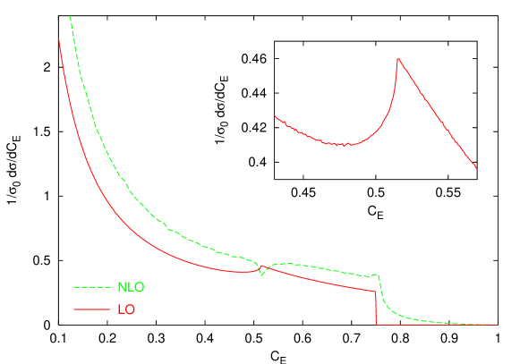
Both the step function at and the square-root behaviour at can be seen in the leading-order distribution for the -parameter in fig. 5. The figure shows also the LONLO result. The pathological nature of the structures which arise at NLO is only partially evident because of the limited resolution of the NLO fixed order terms.
5.2 Other observables
The kinds of patterns that we have discussed can be relevant for other observables — i.e. a smooth (quadratic) maximum in -dimensions leads to a step function in the distribution of , while a smooth maximum along an edge in leads to a square-root behaviour for the distribution around that edge-maximum. The sign of the coefficient of the square-root is the same as the sign of .
It should be noted that features such as step functions (especially at the upper boundary of phase space) can also arise from other kinds of maxima, in particular an edge of constant height (i.e. and ). One such example is the observable whose distribution has a step function at , which is the upper phase-space limit at all orders. Note however that, at least at NLO, there seems to be no higher-order ‘pathological’ behaviour associated with this particular discontinuity of the distribution, perhaps because of the different origin of the discontinuity relative to those discussed above.
Given that these questions are not the main topic of this article, we shall not enter into any more detail. We do however give a summary of the non-smooth features of all the different observables discussed at various stages of this article, table 1.
| Var | Feature | Position |
|---|---|---|
| (LO upper limit) | ||
| (LO upper limit) | ||
| (all-orders upper limit) | ||
| [NB: NLO seems well-behaved] | ||
| (all-orders upper limit) | ||
| (all-orders upper limit) |
6 Speeding-up fixed-order calculations
A necessary element in the comparison of our predictions to data is the matching of the resummed results with fixed-order calculations. However the determination of high-resolution fixed order predictions with a reasonable precision is a significant technical obstacle. High resolution is needed, even when data are coarsely binned, because the shift (or convolution) of the distribution coming from non-perturbative corrections will displace the effective position of the bin boundaries in the perturbative distribution by an a priori unknown amount.
Four programs exist for NLO final-state calculations in DIS: mepjet [37], disent[31], disaster++ [32] and nlojet [38] (not available when this project was started). mepjet has been found [39] to give substantially different results from the other programs (this is unfortunate, because it is the only one with the option of calculating -exchange contributions) and additionally is apparently not suited to the determination of event-shape distributions.
Accordingly at the start of this project, disentand disaster++ were chosen for generating fixed-order distributions. For certain observables however, non-negligible differences had been observed between their predictions [39]. Comparisons to resummations of established [20] that some logarithmically enhanced terms ( in the integrated shape cross-section) were incorrect in disentand the problem has yet to be fixed. This formally leaves us with only disaster++ as an option.
But disaster++ is slow. On a computer with a 2 GHz Pentium IV processor,777Corresponding to SPEC CFP2000 of about 700 [40]. two billion events888Roughly what is used in the coming sections — in finely-binned distributions, statistical errors remain visible, e.g. as for the NLO distribution for the -parameter in fig. 5. represents 50 days’ computing time. Within the standard approach for such programs, one does a run at each pair of experimental interest. The resulting requirement of 400 days’ computing time would have been prohibitive, especially given that at the time when the calculations were carried out, the computers available to us were a factor of two or three slower than those currently on the market.
An alternative approach is based on the observation that for fixed Bjorken-, all that changes when going to different and values is the parton distributions. The matrix element and event-shape calculations remain the same, and there is no need to repeat them. In other words one can exploit factorisation to separate out the structure function () dependence from the rest of the problem. An algorithm which does this (accounting also for Bjorken- dependence) is presented below. It has been implemented in a wrapper program, dispatch, which is available from http://www.lpthe.jussieu.fr/~salam/dispatch/. In practice, with disaster++ it allowed us to calculate distributions at points using only about more computing time than would have been needed for a single point. With disentthe overhead of processing several and points is larger in relative terms (because the matrix-element calculations are quicker in disent), but we still need only about times more computing time for points than for a single one.
6.1 The dispatch algorithm
The algorithm, as currently implemented, is suitable for any observable whose definition, when expressed in the Breit frame, contains no dependence on or on any dimensionful quantity other than through its ratio with (so for example there must be no dependence on the incoming proton momentum, or on the proton remnant, nor any cuts on absolute momenta, nor cuts in the lab frame). Breit-frame event shapes are a good example of such observables.
We shall present our discussion in terms of weighted cross sections , where the weighting function will for example be the value observable itself if one wants to calculate its mean value, or a product of functions so as to obtain the cross section for the observable’s value to be in a certain ‘bin’. For such weighted cross sections we can write
| (33) |
where we have introduced a shorthand for the weighted differential cross section. As is standard for the total cross section we have decomposed the result into transverse+longitudinal () and pure longitudinal () weighted structure functions, . These two weighted structure functions are themselves convolutions of weighted coefficient functions with parton distributions (both of which are vectors in flavour space):
| (34) |
A Monte Carlo program such as disentor disaster++ returns event contributions which, after taking into account the weighting function and averaging over many events with the same value of , correspond to the following function (again a vector in flavour space)
| (35) |
where the refers to the order of perturbation theory. There are two points of interest. Firstly, order by order, is a function only of and , but not of or . Therefore, for a fixed value, the event contributions provided by the Monte Carlo at a single and value are sufficient to allow us to calculate for any and value, through the following convolution
| (36) |
Accordingly the dispatch program uses Monte Carlo events at a single value of and (chosen automatically) to calculate the for a set of and values, all with the same value of .
For comparison to data, a fixed value of is usually not suitable. However the second point of interest in eq. (35) is that all the dependence comes from the linear weighting of the two -independent functions, and . So if we have calculated for two values of , say and , then we can obtain it for any third value, , as follows:
| (37) |
So one simply carries out two dispatch runs at different values and then uses a utility program to combine them with the correct weights so as to correspond to a fixed value of centre of mass energy, .
This means that in principle we have to do two full runs of dispatch. However in many practical situations, for example when comparing to the H1 event-shape distributions in [24] the relevant values all satisfy — choosing a low value for and a high value for it turns out that the weight for the high- run is usually somewhat smaller than that for the low- run, allowing one to generate fewer events at the high- point. As an example, for the fixed-order distributions needed in this paper, we used and , and generated only one tenth of the total number of Monte Carlo events at the higher value. So there is relatively little overhead from generating the second high- point.
7 Inclusion of non-perturbative effects
All of the observables that we consider in this article receive significant non-perturbative contributions. So before comparing our perturbative resummed results to data, it is necessary to correct them for non-perturbative effects. Until a few years ago, this could only be done using the difference between parton and hadron levels in Monte Carlo event generators such as Herwig [41] or Pythia [42]. However such procedures tend to be ill-defined, because of ambiguities in the separation between perturbative and non-perturbative effects. Furthermore, though very successful in describing the data, they involve a number of parameters that must be tuned to the data, as well as many model-dependent assumptions.
When studying event shapes, it can be argued that many of the details of hadronisation (hadron multiplicities, relative abundances of different hadron species, etc.) factor out from the problem, due to the semi-inclusive nature of the observable. This makes it possible to consider the more inclusive aspects of hadronisation analytically, within much simpler and more transparent theoretical approaches.
A general conclusion from such studies is that the dominant hadronisation correction to event shapes is of order [9, 10, 11, 13, 14, 15]. Furthermore there exists a universality hypothesis whereby the size of non-perturbative corrections should involve the product of a calculable, observable-dependent parameter (which we call ) and an a priori unknown parameter (which we will later call ) which should be universal, i.e. independent of the observable and of the process. This hypothesis can be tested by fitting for and in a range of observables and processes.999One may ask why one should be fitting both and , given that is already well determined from other measurements. Two answers exist: firstly one may actually wish to provide an alternative measurement of . Secondly any observable will be subject to higher-order perturbative corrections, and to fix while fitting implies absorbing these higher-order corrections entirely into . Substantial evidence in favour of universality has been obtained with data, using both mean values and distributions [18] and also from mean values of DIS observables [24, 25]. In general distributions tend to give a much more robust test of universality. This is because with mean values one has one data-point for each value and the fit distinguishes and through their different dependences. This procedure can lead to strong correlations between results for and which can mask inconsistencies in the universality hypothesis (or errors in the assumptions behind the calculation of the coefficient ). Distributions of event shapes on the other hand, involve many data points at each value and so have far more discriminatory power. This is one of the main motivations for extending the DIS studies to distributions. It should be kept in mind however that the extension to distributions is not completely without problems, as we illustrate below.
7.1 Means
For mean values non-perturbative effects change the observable by an amount , which within the approach of [11, 43] is assumed to be of the form
| (38) |
where
| (39) |
with an arbitrary infrared matching scale (conventionally taken to be GeV) and the Milan factor [44, 43, 27, 45]. In this approach is interpreted as being the average value of an infrared finite between scales and . The perturbative subtraction terms eliminate the double counting between perturbative and non-perturbative contributions (or equivalently they cancel the perturbative renormalon contribution) and should ensure that the resulting correction is independent of the infrared scale (though itself is not). The renormalisation scale () dependence of the perturbative subtraction terms has the interesting property that it tends to cancel part of the renormalisation scale dependence of the perturbative answer.
7.2 Distributions
For distributions, the situation is more complicated because non-perturbative effects can modify the whole shape of the distribution — this implies a dependence on more than just a single non-perturbative parameter. A very general relation between a perturbative distribution , and the full result including non-perturbative effects, , can be written as
| (40) |
For suitable observables (strictly speaking those that are linear in the momenta of several soft particles), it is argued that in the -jet region non-perturbative effects are independent of and of and can be encoded through a simpler shape function [15, 46],
| (41) |
One can rewrite this in terms of integer moments of ,
| (42) |
where is the derivative of . Consistency with the mean value implies .
The higher moments each involve further non-perturbative unknowns. As discussed in [15, 46, 16] the fact that they multiply implies an expansion in powers of , which in the limit of small should be resummed. In other words formally one needs complete knowledge of the shape function. This requirement is the price one has to pay to ‘gain access’ to all the extra information in distributions as compared to mean values.
It is of interest to consider to what extent it is truly necessary to have complete knowledge of the shape function. Let us take a generic resummation where the normalised integrated distribution is
| (43) |
(for simplicity we neglect all NLL terms) and define . The resummation is valid down to , which translates to . The peak of the distribution
| (44) |
is at , so let us take this as the point up to which we wish to calculate the distribution. To understand the hierarchy of the expansion (42) one needs to know the value of at . This depends strongly on the observable being considered, but can be written fairly generally as
| (45) |
where for and the total and wide-jet broadenings,
| (46a) | |||
| (numerical values are given for ); for the thrust, -parameter and heavy jet mass, and for it is | |||
| (46b) | |||
| and for , and it is | |||
| (46c) | |||
| For there is no analytical solution, but numerically, | |||
| (46d) | |||
So for the broadenings (for which a shape function is in any case not sufficient to describe the non-perturbative effects) the neglect of higher moments might be justifiable down to the peak region, whereas for the observables derived in this paper this is less likely to be true.
Physically, an interesting approximation is to replace the shape function by a -function, which just shifts the perturbative distribution [15, 33],
| (47) |
Remaining terms associated with the full shape function would then correct as follows
| (48) |
While this does not improve the formal convergence of the expansion compared to (42) (we still have an expansion in powers of ) one expects partial cancellation between to improve the actual convergence. Indeed for some observables in , perturbative arguments [16] explicitly suggest and this seems also to be supported by the data.
The approximation of the shift is very powerful, because one has only a single non-perturbative parameter , which is supposed to be universal between different observables, different processes and both mean values and distributions.101010Universality has been postulated (and tested against data) between shape functions (or components thereof) for restricted sets of observables in [47] and [16], though some of the phenomenological aspects of the former analysis have subsequently been argued to be problematic [48] due to a neglect of hadron mass effects. So in what remains of this article we will restrict our analyses to a shift.
7.3 Other considerations
7.3.1 Broadenings
It was stated above that the use of a and -independent shape function held for linear observables. One particular case where this is known not to be true is that of the the broadenings [49, 22] and analogous multi-jet observables [50]. The non-linear dependence of the broadening on multiple emissions has the consequence that the typical non-perturbative correction is roughly proportional to , where is the angle of the current-quark with respect to the photon (or thrust) axis. Because of a correlation between and the broadening, one finds that a non-perturbative correction proportional to . This is taken into account in the fits that follow.
7.3.2 Hadronic mass effects
When testing the universality of corrections, care is needed in the treatment of hadronic mass effects. Most observables are defined in terms of -momenta. Some however, in particular jet masses, depend in their conventional definitions on differences between particle energies and 3-momenta. This leads to universality-breaking corrections (enhanced by powers of ) [48]. Such contributions can be eliminated by suitable redefinitions of the observables. Here we shall consider observables defined in the -scheme, meaning that in the definition of the observable all occurrences of a particle’s energy are replaced by the modulus of its 3-momentum. Of the DIS observables considered in this article, the only one to be modified is the jet mass. Phenomenologically the use of a consistent scheme has been found to be of vital importance in analyses [48, 16] of measurements.
Strictly speaking in the -scheme there remain small universality-breaking mass effects, however they are in practice expected to be negligible, and given that we do not dispose of data in properly universal schemes such as the -scheme or a decay scheme (where measurements are ‘carried out’ after the decay of all massive particles) we make do with -scheme measurements.
Of more concern perhaps is that fact that there can be universal mass effects which could give logarithmic corrections to the -dependence of power-suppressed effects. Because we are not able to estimate the absolute normalisation of these universal mass effects (or even their sign) it is not a priori clear how to eliminate them. However it should be noted that even ‘traditional’ corrections may be subject to anomalous dimension-like corrections, coming from single-logs associated with the fact that soft particles are emitted not off a bare current, but rather off a ‘dressed’ pair: i.e. the emits large angle soft gluons with ’s ranging between between and (giving powers of ) and soft gluons with transverse momenta of order are emitted coherently off that whole ensemble. The approximate rapidity-independence of the ‘dressing’ ought to ensure however that universality is not broken.
A final point relevant to all these anomalous-dimension-like corrections (whether associated with mass effects or coherent emission off dressed pairs) is that in distributions, the single logs may acquire a dependence on the value of the observable. For example, for a continuously-global observable such as one schematically expects occurrences of in corrections to the mean, to be replaced by in distributions, because the hardest (perturbative) large-angle emission must have a scale which is smaller than . For non-global and discontinuously global observables, the modification is likely to be more complex.
In any case it should be emphasised that even the first order correction term, , has yet to be calculated for any observable. So in the phenomenological analyses that follow later we shall ignore these complications.
8 Resummation: impact and uncertainties
8.1 Effect of resummation and matching
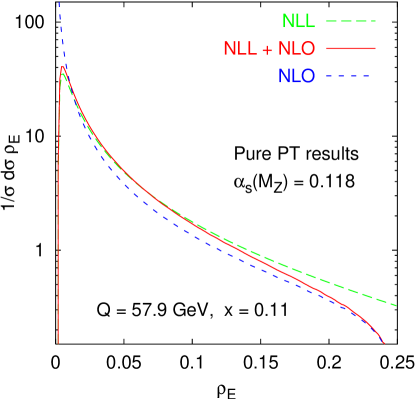
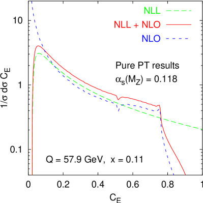
In figure 6 we show pure NLO predictions, pure NLL predictions (with modified logs) and matched NLO-NLL results ( scheme, as described in [22]) for the distributions of two observables: and the -parameter. Aside from leading to the appearance of a Sudakov peak in the exclusive limit, the resummation has a non-negligible (-) effect even for intermediate values of the observable, where the logarithms being resummed, while not formally large, can still be numerically significant. In many cases this will be the region used for fits.
It is interesting also to examine the region where the value of the observable is large. For the jet mass we see that the matched-resummed curve coincides almost exactly with the NLO curve close to the kinematical limit , where the leading contribution is . The situation for is more complicated because beyond the leading contribution is . There one sees that the NLLNLO curve behaves very differently from the pure NLO curve. This is almost certainly an artefact of the matching procedure, which is not intended to be used in situations where the leading term is not of order .
8.2 Choice of default -scale for the logs
In a resummation which is truncated to some fixed logarithmic order (e.g. NLL) there is an ambiguity associated with the choice of logarithm to be resummed. For example for the jet mass we resummed , while for the thrust we took . The different factors were motivated by the kinematical relation between the jet mass and the thrust, derived in section 2. But we could just as easily have chosen to resum and — the single-logarithmic contribution in terms of these redefined logarithms would have a different functional form, but the overall answer would be the same to NLL accuracy.
In [22] we formalised this ambiguity by introducing an “-scale” parameter, allowing us to redefine the logarithm to be resummed,
| (49) |
where is the default coefficient in the numerator of the logarithm (, , ).
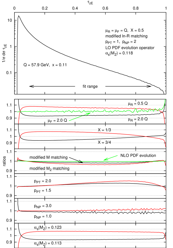
Having introduced the parameter one should establish a consistent procedure for setting it for a range of variables. We adopt the convention of choosing the default such that the resulting coefficient only contains terms associated with hard collinear contributions (the yellow bands in fig. 1). For , , and (as for all the usual resummations) this corresponds to , while for , and for , .
8.3 Summary of uncertainties
There are a number of potential sources of uncertainty on matched resummed event-shape distributions, essentially associated with unknown higher-order contributions.
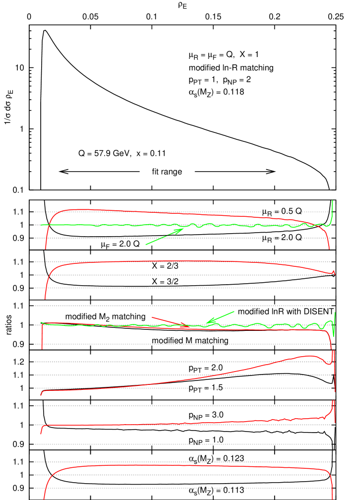
We can obtain an indication of the size of higher-order corrections in a number of ways, and the effects are illustrated in figs. 7 and 8. These figures show the matched resummed distributions ( and respectively) for default choices of parameters, matching procedures and non-perturbative corrections, together with the ratio to the default distributions when varying different scale and matching parameters.
The first ratio plot shows the effect of varying by a factor of two, with the effect being at about the level, and slightly larger for . Also shown is the effect of taking (with ), which is in comparison negligible — it should be kept in mind of course that at this value the scale dependence of the structure function is quite weak, however it is generally true that the resummation is much more sensitive to than to .
The next plot shows the effect of varying . The range to choose for is somewhat arbitrary (as is the range for the renormalisation scale). The question has been investigated in some detail in [51] for event shapes, where the effect of variations in has been compared analytically to known higher-order effects, for example to the size of the subleading () term. As would be expected a suitable range is somewhere between to and to , with the actual range in [51] chosen to be between and . This particular range has the feature in event shapes that the overall impact of the variation is similar to that of the (standard) variation, the purpose of the variation then in part being to have access to an alternative functional form for the uncertainty. This is also the range used in figs. 7 and 8 and we note that here too, the effect is of the same order as that from variation, though the functional dependence on the observable is somewhat different.
Next we investigate the effect of different kinds of matching, described in [22], related to analogous procedures in [1]. In the default matching ( is given by eq. (13)) is adjusted to have the correct expansion and then exponentiated to give the integrated distribution. In matching, one calculates the difference between the expansion of and the exact distribution at first and second order in , and this difference (multiplied by , so as to ensure correct behaviour in the limit, essentially the condition that for ) is then added to . Actually the difference between first order resummed and exact distributions will automatically go to zero for — it is only at second order that this does not happen (because we do not know the values of the and terms of the resummation: in these are usually fitted to the fixed order, but this is not feasible in DIS). Accordingly the multiplication by is only really necessary at second order, which then gives matching. The plot shows the effect of changing to and matchings, and we see that it is small.
Though not strictly an uncertainty, for we show additionally the effect of replacing the fixed order calculation from disaster++ with that from disent. The effect turns out to be negligible. The same is found to be true for most of the other observables as well, despite the fact that an examination of the logarithmic structure does in general reveal differences at . There are two main reasons why the the effect of changing to disentis relatively small. Firstly the largest differences between disentand disaster++ are in the gluon induced channel, which is relatively suppressed at this value. Secondly because of the structure of , and matching, any differences between the disentdistribution and the correct logarithmic structure are multiplied by a Sudakov form factor, and so are suppressed by the matching procedure.111111We note that in -type matching procedures (not easily used given the currently available tools in DIS), one finds significant differences at lower and lower values of the observables. Accordingly in some instances in this paper, where for technical reasons we did not have suitable disaster++ fixed-order results, we use instead disentresults (one such case is in the estimates of the dependence).
In the case of , which involves the evaluation of the PDFs at a scale we show the effect of changing from LO to NLO PDF evolution (as explained in [22], at single-log accuracy both are equally valid, though for the matching and terms to be correct, the starting distribution at scale must be an NLO parton distribution). At this value of , and scaling violations are small, and as a result there is very little effect in switching to NLO PDF evolution. At other values (with correspondingly different values), the effects are visible, but still relatively unimportant.
Another aspect of matching is the use of modified logs,
| (50) |
where, in the original formulation [1] was 1. This modification of the logarithms is necessary to ensure that goes to the correct value (total cross section minus cross section for ) at and in some cases additionally that the distribution goes to zero at . This modification introduces terms involving products of and . Such terms are known to exist (see e.g. [2]). However only terms with are expected to be present, so we restrict . Two possible values are shown in figs. 7 and 8, and in the region of small variable, the dependence is fairly weak, though it increases, especially for towards the upper kinematical limit.
Analogously, one can modify the power correction so that it vanishes at the upper limit of the observable. This is especially relevant for observables whose distribution remains finite at the upper limit. The modification that we choose [22] is
| (51) |
By default we have taken (on the grounds that we wish to modify the simple picture of a shift as little as possible). We see that the effect of varying it between and is small.
For reference, the last ratio plot shows the effect of varying by . It enables one to make an order of magnitude estimate of the relation between uncertainties on the distributions and a corresponding uncertainty in a fit for . We point out however that when carrying out a simultaneous fit for both and , the situation is more complicated because of the correlation between the two quantities.
9 Comparison to data
In this section we fit a range of resummed DIS event-shape distributions to H1 data [24]. It would be beyond the scope of our expertise to carry out a ‘proper’ fit, taking into account for example full correlations of the systematic errors. Rather the results of this section should be taken as indicative, and in particular the errors on our fit results are likely to be underestimated.121212For those wishing to carry out a more sophisticated analysis, the programs used to calculate the matched resummed distributions are available from http://www.lpthe.jussieu.fr/~salam/disresum/.
We shall examine all the measured event shapes, with the jet mass taken in the scheme, as discussed in section 7.3.2.131313We thank Uli Martyn for providing us with the numerical values for the distribution of this observable. The data is binned in as shown in table 2.
Formally when calculating the theoretical distribution, one ought to divide the and ranges into small sub-bins, calculate the full matched and non-perturbatively shifted distribution in each sub-bin and then recombine to obtain results for the whole bin. The main practical limitation on this approach is that of calculating the fixed-order perturbative distributions for all the sub-bins, which even with the methods of section 6 would probably have required computing resources beyond those available to us.141414The problem could probably be rendered tractable using an adaptation of methods described in [52]. Instead we simply calculate the distributions for the mean and values as given in table 2. Both the theoretical and experimental distributions are normalised to the total cross section for the energy in the current hemisphere to be larger than .
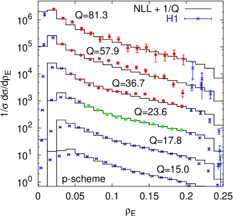
The fits will involve two free parameters: and the non-perturbative parameter with . We aim to learn several things from them: we wish to verify the consistency of (and ) with other measurements (from means and distributions and DIS means). And we would also like to check that the fit results are consistent across a range of values. To accomplish this we will carry out two sets of fits, one for all data with and a second one with additionally the bin . The region on its own has a statistical weight slightly larger than the combined region.
The upper limit on the variable in the fit is chosen to be below the maximum value for the observable (which in some cases coincides with the all-orders maximum), because beyond this point the fixed-order distribution is known only at leading order and because the current matching procedures make little sense in steeply falling regions beyond the maximum. The lower limit on the variable (applied to the bin centre) is chosen to scale as . The coefficient of the scaling is taken larger for observables with larger power corrections. In some cases at the highest point even the lowest variable-bin is included. While at first sight it may look like one is therefore probing the distribution down to zero (which would be unsafe), what one is actually doing in such a bin is probing the integrated distribution at the upper boundary of the bin, which is potentially acceptable as long as that upper boundary is in the immediate neighbourhood, or to the right of the maximum of the distribution.
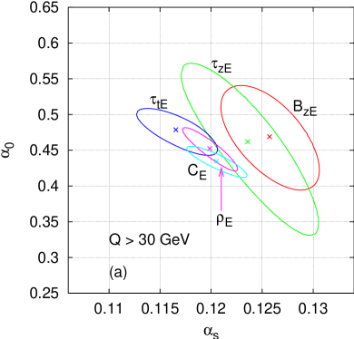
The fitted distributions are compared to data in figures 9 () and 10 (, , and ).151515We note that for the -parameter we have used disentrather than disaster++ fixed-order predictions — this is for technical reasons and in light of the discussion in section 8.3 it is not expected to affect the results significantly. Only the red (round) points have been used in the fit (the green squares correspond to those points that will additionally be used in the fit for GeV). The -sigma contours of the fit results are shown in figure 11a and the numerical results together with the values are given in table 3.
One sees remarkably good consistency between the observables, with the possible exception of the broadening, whose value exceeds the world average by just over a standard deviation (but one should keep in mind that our neglect of correlations between errors may lead to an underestimate of the errors). The results are also in very good agreement with those from mean values (see for example the -scheme results of [48]). Furthermore they are reasonably compatible with results from fits to means in DIS [24, 25] and from distributions in [18], though in these two cases the internal consistency between fits to different observables is not perfect.
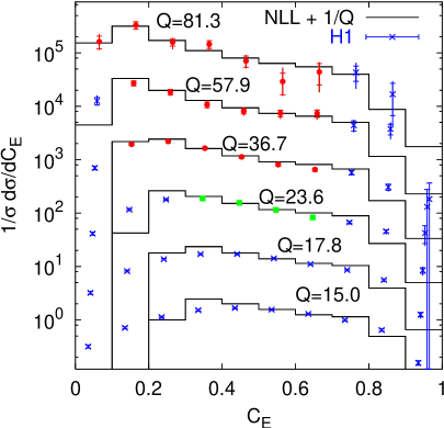
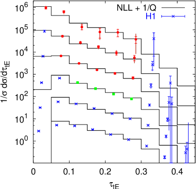
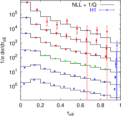
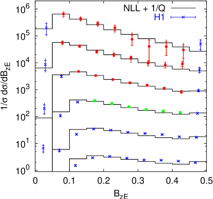
Returning to the DIS distributions, for all variables except the results are reasonable. Looking at the comparison between the data and theoretical predictions, figure 9, there seem to be problems in the central region of the distribution for for the GeV bin and also somewhat for the GeV bin. There is no evidence for any such discrepancy in the bins immediately above and below, so it is a problem which needs to be better understood.
| d.o.f. | |||
|---|---|---|---|
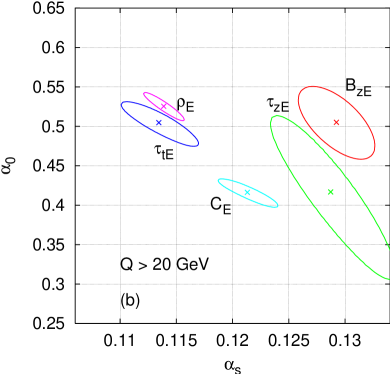
It is interesting also to examine what happens when we extend our fits to lower . Figure 11b shows the fit results when one additionally includes the GeV bin (the green points of figures 9 and 10). Because of the larger number of events at lower values, the statistical weight of the GeV data points is comparable to and sometimes even larger than that from all the higher- bins combined. Its inclusion leads to a significant reduction in the consistency between different observables, though is still variable-independent to within .
The decrease in consistency as one one goes to lower , both between observables and compared to the world average for , could well be due to the relatively more important role of higher order contributions at lower , whether in the form of or non-perturbative effects or NNL perturbative contributions. It would be of considerable interest to have higher-precision data at the larger values so as to be able to trace such effects in a continuous fashion and perhaps even identify their origin.
In this context we note that the apparent more limited consistency between observables in fits to DIS mean values [24, 25] might be due to the inclusion of very low data. To establish whether this is truly the explanation, there is a need for higher statistics in order to be able to carry out a meaningful fit using just the higher- mean values.
A point of some interest is that it is the observables measured with respect to the photon axis that are less consistent with the world average for (giving larger values). The fact that these observables are directly sensitive to the transverse momentum of the incoming parton leads one to wonder whether we are seeing the early onset of some small- effect or of an ‘intrinsic’ transverse momentum of the proton. An extension of measurements and theoretical predictions to a wider range of observables might therefore be of interest, in particular for observables which exist in ‘thrust-axis’ and ‘photon-axis’ variants (in analogy to the two thrusts), such as the broadenings (i.e. as well as ) and the thrust majors. Theoretical predictions for the latter would probably need to use the semi-numerical methods developed in [6].
| pure NLO | No NG logs | |||
| — | — | |||
As an aside, for illustrative purposes we also examine what impact the resummations themselves have on the fit results. In the left-hand part of table 4 we show the change in the , fit results (with GeV) where the matched resummed perturbative part has been replaced by the pure NLO result, while keeping the fit-range fixed. The results clearly become incompatible with the world average, at about the – level, though for all variables other than (where we have technical problems with the fit) the values remain reasonable. The values remain more or less consistent with our expectations (except for ).
In the right-hand part of table 4 we show the changes in and that follow from neglecting non-global logarithms in the resummed component of matched, power-corrected fits to the data. One sees effects of between and on for non-global variables and much less of an effect for the discontinuously global . The non perturbative parameter is in contrast relatively insensitive to non-global effects. It should be kept in mind that in these fits the matching in any case fixes up the term, so it is only the effect of terms with (about half the total effect) that is reflected.
Finally, returning to the normal matched resummed fits, we should emphasise that we have not considered the impact of the uncertainties discussed in section 8.3. These should be examined in future studies, together with an analysis of the stability of the results with respect to variations in the fit ranges (with the current statistics this is difficult unless one includes lower- data), and of the impact of integrating the predictions over the whole bin rather than just taking them at the mean of the bin. Finally if and when the tools for fixed-order calculations including exchange and interference become available, then it would be useful to evaluate their impact on the results (the resummations themselves are not affected, but the constant terms and matching are).
10 Conclusions
The study of DIS event shapes has been largely motivated by the vast amount of HERA data that has become available over the past few years and the notable success of a similar study for variables. While mean values were the first properties of DIS event shapes to be examined theoretically, interest is shifting to the study of differential distributions for which there are over 500 data points available from H1. Here we shall summarise the developments that have taken place during the entire course of our study involving DIS event shape distributions.
The project of studying the DIS distributions implies the calculation of resummed predictions, matched to fixed order ones to enable one to study the distribution over a wide enough range of values. While it was initially believed that the DIS resummed predictions would offer relatively few extra complications, given the techniques in place for variables (the development of which spanned nearly a decade) and the similarities in definitions of the event shapes, this turned out not to be the case.
From a purely theoretical viewpoint the first complication encountered was that of the different treatment, of collinear logarithms associated with the parton distribution functions and the presence of an incoming gluon channel which features were naturally absent in the cases. In [20, 22] we demonstrated that for boson axis variables such collinear radiation (including the incoming gluon channel) is associated with a change in scale of the structure function where denotes the variable. This variable dependence of the scale of the structure function had been encountered prior to work on DIS event shapes in for example the study of the transverse momentum distribution of a vector boson produced in hadron-hadron collisions (see e.g [53]).More recently it was also established to be present in certain three jet event shapes, both in DIS and hadron-hadron collisions, for which we refer the reader to the last two items of [50]. In contrast for two (1+1) jet DIS event-shape variables not defined using the boson axis, such as those discussed in the present article, one just needs to factorise the parton densities as for a cross section and the relevant scale of the PDFs remains .
While straightforward to understand theoretically, the presence of parton distributions, different incoming partonic channels, transverse and longitudinal components of the result with their different dependences and the presence of anomalous dimension matrices rather than simple numbers in the coefficients of certain single logarithmic terms, creates considerable problems of notation and particularly implementation. We dealt with and explained most of these issues in Refs. [20, 22] and therefore in this article presented the results in only a skeletal form.
One other problem that we encountered during the course of our study was the lack of a suitable fixed order Monte Carlo program with which to combine (match) our results. While both disentand disaster++ were available to us, we found that our analytical resummations, expanded to NLO, indicated disagreement, in certain terms, with disentand compatibility with disaster++. We would therefore have preferred to use disaster++ for our purposes but for the fact that it was slow. We therefore developed a package (dispatch), described in Sec. 6, that considerably speeds up (by an order of magnitude) disaster++, making it possible to obtain results for several points with a precision which, from the point of view of computing time, would have been unfeasible previously.
While on the subject of fixed order computations we also developed several matching schemes to combine our results with those from NLO Monte Carlos [22]. While some of these (e.g ) involved extensions and generalisations of the corresponding procedures [1] (albeit more subtle in the DIS case) we also proposed, for the first time, multiplicative matching schemes ( and matching) [22].
Another development that we made in the course our study of DIS event shapes was the writing of our own PDF evolution code. This was necessitated by for example the need for flexibility in the evolution, specifically to fit using the same value for all components of the result rather than have part of the result ‘contaminated’ by the used in the standard (e.g. [54, 55]) PDF sets. Also it was found that for our particular variables, there were problems arising from the non-smoothness of the interpolation procedure used in [54]. Our PDF evolution code enabled the discovery of bugs in the standard evolution codes (MRST and CTEQ), which have as a result been fixed [56, 57].
Technical spin-offs apart, one important theoretical discovery made during our investigation of DIS event shapes turned out to be that of non-global logarithms. These have been discussed in great detail elsewhere [28, 29], while in the current article we have considered their extension to discontinuously global variables, correcting (phenomenologically relatively unimportant) omissions in [20, 22].
Lastly, we come to the original aim of this work: the comparisons with data. These give a strong boost to the idea of a universal non-perturbative extension to the standard coupling . In the case of most variables we find that the agreement with data at intermediate to larger values is remarkable down to very small values of the variables in question. The and values obtained by fitting our results to H1 data are in general consistent with the world average and values respectively. From the viewpoint of theory, the noticeable worsening of the description that occurs at low values is an area that may require further investigation. On the experimental front, data from ZEUS is eagerly awaited as is high luminosity H1 data. This apart, a proper error analysis in the fits to existing data should also be carried out. Lastly the impact of the various subleading uncertainties involved in our resummation on actual fits to the data should also be examined.
Acknowledgments.
We wish to thank Vito Antonelli for discussions during the initial stages of this paper. One of us (GPS) also wishes to thank members of the LEP QCD working group for discussions related to -scale dependence. The fixed-order calculations used here were obtained in part using computer facilities at CERN and at the universities of Milano and Milano-Bicocca. We also wish to thank Uli Martyn, Klaus Rabbertz and Thomas Kluge for helpful comments and for providing us with the H1 data in numerical form, and Yuri Dokshitzer, Einan Gardi and Johann Rathsman for numerous stimulating discussions.Appendix A Resummed results
The results for the quark and gluon jet mass cross-sections and were first derived in [1]. They can be expressed as below
| (52) |
where the “radiator” is given to NLL accuracy by
| (53) |
with being the derivative
| (54) |
where we have used and in the derivative have dropped subleading (NNLL) pieces involving the derivative of .
The functions and are listed below
| (55) |
and
| (56) |
In the above results the function coefficients and are defined as
| (57) |
and the constant is given by
| (58) |
For the gluonic contribution one only requires the leading log piece of the answer, since this contribution is already suppressed by a factor of which comes from the probability of having a hard gluon in the current hemisphere:
| (59) |
where is identical to the corresponding quark result (55), provided one replaces the quark colour charge by .
Finally we come to the non-global resummation factor . This was parameterised as below in Ref. [28]
| (60) |
with
| (61) |
with as above and
| (62) |
The above parameterisation takes into account the exact leading order result computed in [28] and all subsequent orders in the large limit (i.e. neglecting contributions ). The above parameterisation ought to be be accurate to within a few percent for which corresponds to (and to within a fraction of a percent up to which remains beyond the largest values of probed phenomenologically).
Appendix B Constant pieces
The various coefficient functions that we shall require can be written in the notation where shall denote the transverse or longitudinal piece, the index shall signify the incoming particle and the upper index shall denote the hard particle in off which we perform the resummation to obtain the form factor .
One has (multiplied in (13) by )
| (63) |
We find it convenient to introduce the function which is the whole constant piece (sum of contributions from current quark and gluon pieces) that appears in the one-loop calculation of the probability of having jet mass above . From and we can extract via the relation The function is
| (64) |
Analogously one has
| (65) |
and
| (66) | ||||
| (67) | ||||
| (68) |
The thrust variable has identical coefficient functions to those listed above for the the jet mass. For the C parameter the only difference is in the piece (which also affects ) where one needs to add the term to the term listed above.
Note that in order to go from the coefficient functions above to the Bjorken dependent constant pieces relevant to we have to take pieces with the appropriate weights, convolute the functions above with the parton density functions and normalise to the Born value for . Incoming quark pieces need to be convoluted with where the sum runs over quarks and antiquarks, and convolutions are defined as
| (69) |
Similarly incoming gluon pieces need a convolution with where is the gluon density. To then go to the coefficient functions used in eq. (13) one uses relations such as
| (70) |
where is Bjorken-.
Finally we recall that as in [20], the coefficient functions are given in the DIS scheme. To go to another scheme one should add to and the corresponding coefficient functions in that scheme.
References
- [1] S. Catani, L. Trentadue, G. Turnock and B. R. Webber, Nucl. Phys. B 407 (1993) 3; S. Catani, G. Turnock, B. R. Webber and L. Trentadue, Phys. Lett. B 263 (1991) 491.
- [2] S. Catani, G. Turnock and B. R. Webber, Phys. Lett. B 295 (1992) 269.
-
[3]
S. Catani, Yu. L. Dokshitzer, F. Fiorani and B. R. Webber,
Nucl. Phys. B 377 (1992) 445;
- [4] S. Catani and B. R. Webber, Phys. Lett. B 427 (1998) 377 [arXiv:hep-ph/9801350].
- [5] Y. L. Dokshitzer, A. Lucenti, G. Marchesini and G. P. Salam, JHEP 9801 (1998) 011 [arXiv:hep-ph/9801324].
- [6] A. Banfi, G. P. Salam and G. Zanderighi, JHEP 0201 (2002) 018 [arXiv:hep-ph/0112156].
- [7] S. Catani, Yu. L. Dokshitzer and B. R. Webber, Phys. Lett. B 322 (1994) 263.
-
[8]
See for example:
P. D. Acton et al. [OPAL Collaboration],
Z. Phys. C 59 (1993) 1;
P. Abreu et al. [DELPHI Collaboration], Z. Phys. C 73 (1997) 229;
O. Biebel, P. A. Movilla Fernandez and S. Bethke [JADE Collaboration], Phys. Lett. B 459 (1999) 326 [arXiv:hep-ex/9903009]. - [9] A. V. Manohar and M. B. Wise, Phys. Lett. B 344 (1995) 407 [arXiv:hep-ph/9406392].
- [10] B. R. Webber, Phys. Lett. B 339 (1994) 148 [arXiv:hep-ph/9408222].
- [11] Y. L. Dokshitzer and B. R. Webber, Phys. Lett. B 352 (1995) 451 [arXiv:hep-ph/9504219].
- [12] Y. L. Dokshitzer, G. Marchesini and B. R. Webber, Nucl. Phys. B 469 (1996) 93 [arXiv:hep-ph/9512336].
- [13] R. Akhoury and V. I. Zakharov, Phys. Lett. B357 (1995) 646; R. Akhoury and V. I. Zakharov, Nucl. Phys. B465 (1996) 295;
- [14] M. Beneke and V. M. Braun, Nucl. Phys. B 454 (1995) 253 [arXiv:hep-ph/9506452].
- [15] G. P. Korchemsky and G. Sterman, Nucl. Phys. B437 (1995) 415;
- [16] E. Gardi and J. Rathsman, Nucl. Phys. B 609 (2001) 123 [hep-ph/0103217]; E. Gardi and J. Rathsman, hep-ph/0201019.
- [17] For a review, see M. Beneke, Phys. Rept. 317 (1999) 1 [arXiv:hep-ph/9807443].
- [18] See for example P. A. Movilla Fernandez, S. Bethke, O. Biebel and S. Kluth, Eur. Phys. J. C 22 (2001) 1 [arXiv:hep-ex/0105059].
-
[19]
J. R. Ellis, V. A. Khoze and W. J. Stirling,
Z. Phys. C 75 (1997) 287
[arXiv:hep-ph/9608486];
V. A. Khoze and W. J. Stirling, Z. Phys. C 76 (1997) 59 [arXiv:hep-ph/9612351];
C. F. Berger, T. Kucs and G. Sterman, Phys. Rev. D 65 (2002) 094031 [arXiv:hep-ph/0110004];
C. F. Berger et al., in Proc. of the APS/DPF/DPB Summer Study on the Future of Particle Physics (Snowmass 2001) ed. R. Davidson and C. Quigg, arXiv:hep-ph/0202207. - [20] V. Antonelli, M. Dasgupta and G. P. Salam, JHEP 0002 (2000) 001 [arXiv:hep-ph/9912488].
- [21] V. Antonelli, M. Dasgupta and G. P. Salam, J. Phys. G 26 (2000) 658 [arXiv:hep-ph/9910343].
- [22] M. Dasgupta and G. P. Salam, Eur. Phys. J. C 24 (2002) 213 [arXiv:hep-ph/0110213].
- [23] C. Adloff et al. [H1 Collaboration], Phys. Lett. B 406 (1997) 256 [arXiv:hep-ex/9706002].
- [24] C. Adloff et al. [H1 Collaboration], Eur. Phys. J. C 14, 255 (2000) [Addendum-ibid. C 18, 417 (2000)] [arXiv:hep-ex/9912052].
- [25] G. J. McCance [ZEUS collaboration], hep-ex/0008009.
- [26] M. Dasgupta and B. R. Webber, Eur. Phys. J. C 1 (1998) 539 [arXiv:hep-ph/9704297].
- [27] M. Dasgupta and B. R. Webber, JHEP 9810 (1998) 001 [arXiv:hep-ph/9809247].
- [28] M. Dasgupta and G. P. Salam, Phys. Lett. B 512 (2001) 323 [arXiv:hep-ph/0104277].
- [29] M. Dasgupta and G. P. Salam, JHEP 0203 (2002) 017 [arXiv:hep-ph/0203009].
- [30] S. Catani and B. R. Webber, JHEP 9710 (1997) 005 [arXiv:hep-ph/9710333].
- [31] S. Catani and M. H. Seymour, Nucl. Phys. B 485 (1997) 291 [Erratum-ibid. B 510 (1997) 503] [arXiv:hep-ph/9605323].
- [32] D. Graudenz, arXiv:hep-ph/9710244.
- [33] Y. L. Dokshitzer and B. R. Webber, Phys. Lett. B 404 (1997) 321 [arXiv:hep-ph/9704298].
- [34] S. Catani and L. Trentadue, Nucl. Phys. B 353 (1991) 183.
- [35] S. Catani, B. R. Webber and G. Marchesini, Nucl. Phys. B 349 (1991) 635.
- [36] A. Banfi, G. Marchesini and G. Smye, arXiv:hep-ph/0206076.
- [37] E. Mirkes and D. Zeppenfeld, Phys. Lett. B 380 (1996) 205 [arXiv:hep-ph/9511448].
- [38] Z. Nagy and Z. Trocsanyi, Phys. Rev. Lett. 87 (2001) 082001 [arXiv:hep-ph/0104315].
- [39] G. McCance, NLO program comparison for event shapes, in Monte Carlo Generators for HERA Physics Proceedings, DESY-PROC-1999-02, also hep-ph/9912481.
- [40] Standard Performance Evaluation Corporation, http://www.spec.org/.
- [41] G. Marchesini, B. R. Webber, G. Abbiendi, I. G. Knowles, M. H. Seymour and L. Stanco, Comput. Phys. Commun. 67 (1992) 465.
- [42] T. Sjostrand, Comput. Phys. Commun. 82 (1994) 74.
- [43] Y. L. Dokshitzer, A. Lucenti, G. Marchesini and G. P. Salam, JHEP 9805 (1998) 003 [hep-ph/9802381].
- [44] Y. L. Dokshitzer, A. Lucenti, G. Marchesini and G. P. Salam, Nucl. Phys. B511 (1998) 396 [hep-ph/9707532] erratum ibid. B593 (2001) 729.
- [45] M. Dasgupta, L. Magnea and G. Smye, JHEP 9911 (1999) 025 [hep-ph/9911316]; G. E. Smye, JHEP 0105 (2001) 005 [hep-ph/0101323].
- [46] G. P. Korchemsky, G. Oderda and G. Sterman, presented at 5th International Workshop on Deep Inelastic Scattering and QCD (DIS 97), Chicago, IL, April 1997 hep-ph/9708346; G. P. Korchemsky and G. Sterman, Nucl. Phys. B 555 (1999) 335 [hep-ph/9902341].
- [47] G. P. Korchemsky and S. Tafat, JHEP 0010 (2000) 010 [arXiv:hep-ph/0007005].
- [48] G. P. Salam and D. Wicke, JHEP 0105 (2001) 061 [arXiv:hep-ph/0102343].
- [49] Y. L. Dokshitzer, G. Marchesini and G. P. Salam, Eur. Phys. J. directC 3 (1999) 1 [arXiv:hep-ph/9812487].
- [50] A. Banfi, G. Marchesini, Y. L. Dokshitzer and G. Zanderighi, JHEP 0007 (2000) 002 [hep-ph/0004027]; A. Banfi, Y. L. Dokshitzer, G. Marchesini and G. Zanderighi, Phys. Lett. B 508 (2001) 269 [hep-ph/0010267]; A. Banfi, G. Marchesini, G. Smye and G. Zanderighi, JHEP 0108 (2001) 047 [hep-ph/0106278]; A. Banfi, G. Marchesini, G. Smye and G. Zanderighi, JHEP 0111 (2001) 066 [arXiv:hep-ph/0111157].
- [51] LEP QCD working group, in preparation.
- [52] D. A. Kosower, Nucl. Phys. B 520 (1998) 263 [arXiv:hep-ph/9708392].
-
[53]
J.C. Collins and D.E. Soper, Nucl. Phys. B 193 (1981) 381;
ibid., Nucl. Phys. B 197 (1982) 446;
ibid., Nucl. Phys. B 213 (1982) 545 (erratum);
J. Kodaira and L. Trentadue, Phys. Lett. B 112 (1982) 66;
ibid., Phys. Lett. B 123 (1983) 335;
J.C. Collins, D.E. Soper and G. Sterman, Nucl. Phys. B 250 (1985) 199. -
[54]
A. D. Martin, R. G. Roberts, W. J. Stirling and R. S. Thorne,
Eur. Phys. J. C 14 (2000) 133
[hep-ph/9907231];
- [55] H. L. Lai et al. [CTEQ Collaboration], Eur. Phys. J. C 12 (2000) 375 [hep-ph/9903282];
- [56] A. D. Martin, R. G. Roberts, W. J. Stirling and R. S. Thorne, Eur. Phys. J. C 23 (2002) 73 [arXiv:hep-ph/0110215].
- [57] J. Pumplin, D. R. Stump, J. Huston, H. L. Lai, P. Nadolsky and W. K. Tung, JHEP 0207 (2002) 012 [arXiv:hep-ph/0201195].