On the chirality of quark modes

Abstract

A model for the QCD vacuum based on a domainlike structured background gluon field with definite duality attributed to the domains has been shown elsewhere to give confinement of static quarks, a reasonable value for the topological susceptibility and indications that chiral symmetry is spontaneously broken. In this paper we study in detail the eigenvalue problem for the Dirac operator in such a gluon mean field. A study of the local chirality parameter shows that the lowest nonzero eigenmodes possess a definite mean chirality correlated with the duality of a given domain. A probability distribution of the local chirality qualitatively reproduces histograms seen in lattice simulations.

I Introduction

In a previous paper KaNe01 we formulated a model which characterises the QCD vacuum by a “lumpy” distribution of field strength and topological charge density. For lack of a better name we shall refer to the model as “the domain model”. The formulation is given concretely in terms of a partition function which describes a statistical ensemble of domains, each of which is characterised by a set of internal parameters associated with the mean background gluon field, and the internal dynamics are represented by fluctuation fields. Correlation functions in this model can be calculated by taking the mean field into account explicitly and decomposing over the fluctuations. We briefly review the details and assumptions behind the model in the next section but state here unambiguously that the “domains” in question are assumed to be purely quantum in nature. They are not semi-classical solutions of Yang-Mills theory and are not argued to exist as topologically stable classical configurations, rather they seek to characterise the average bulk properties of the ensemble of fields that determine the gluonic vacuum. In particular, it is not assumed that the topological charge associated with a domain should be an integer. The rationale of such an extremely simplified construction can be understood as an attempt to implicitly incorporate effects of the presence of singular pure gauge configurations in the QCD Euclidean functional integral into a practical calculational scheme with a mean field description of the QCD ground state. A self-consistent mean field approach requires nonperturbative calculation of the free energy as a functional of the mean field whose minima should determine its form, but this is beyond the reach of analytical methods. Nevertheless there is an accumulation of semi-qualitative arguments KaNe01 in favour of the ansatz for the mean field we have chosen.

In the gluonic sector the model depends on two parameters, a mean field strength per domain $B$ and a mean size for domains $R$, which is sufficient for an adequate description of the pure glue characteristics of the QCD vacuum – the gluon condensate, topological susceptibility, and string tension. The Wilson loop in such a gluonic background was found to exhibit an area law dependence for large loops. Thus a confinement of static fundamental charges is captured by the model; some dynamical gluon degrees of freedom turn out also to be non-propagating. The absolute value of underlying average topological charge per domain was determined to be approximately $q=0.15$ and the density of domains to be as high as 42 fm^-4. Although tentative signals of spontaneous chiral symmetry breaking were also obtained in KaNe01 , a more rigorous consideration of the fermionic spectrum and eigenmodes as well as calculation of the quark determinant is required, which was missed in KaNe01 .

In this paper we solve the eigenvalue problem for the Dirac operator for the gluonic background and boundary conditions adopted in the model and examine the chirality properties of the eigenmodes. This is a necessary step for checking the status of chiral symmetry breaking in the domain model. But in view of recent lattice results this problem is valuable also in its own right.

There are strong hints in lattice Monte-Carlo simulations at intermediate-range structures in individual gluon configurations once fluctuations are filtered out by some means. For example, cooling or relaxation algorithms are well established now cooling , and can reveal instantonic like structures after several sweeps of a given lattice configuration. However, as these algorithms are designed precisely to locally minimise the action, it is natural they should bring objects with integer topological charge into relief. Alternately, and more relevant to the present work, low-lying and zero-modes of the massless Dirac operator can be used as a probe of long-range gluonic structures fermionmodes although only recently did this become more reliable with lattice fermions with good chirality properties. For example, exact index theorems are found to be satisfied on the lattice Zha02 and the zero modes are seen to precisely correlate with instantonic structures in the raw lattice configuration, in the absence of cooling EdH02 . However, the exact zero modes of any finite volume simulation cannot be those relevant to spontaneous chiral symmetry breaking, rather the discrete spectrum of low-lying non-zero modes should, in the infinite volume limit, go over to a continuous band at zero, saturating the Banks-Casher relationship BaC80 . Such modes are sometimes called “pseudo zero modes”. Low-lying non-zero modes with strong signs of chirality in regions of high action and topological charge densities would be a tool for identification of the properties of gluonic configurations relevant to chiral symmetry breaking. Indeed, after an initial negative result Hor02 , recent results have emerged showing precisely this: low-lying non-zero modes of the overlap Dirac operator which seem to accrue to topological structures and exhibit strong chirality, as measured by the local parameter $X$ defined by

$$\tan\left(\frac{\pi}{4}(1-X(x))\right)={{|\psi_{-}(x)|}\over{|\psi_{+}(x)|}},$$ (1)

in regions where the probability density ${\psi}^{\dagger}(x)\psi(x)$ of these modes is maximal EdH02 . The verification of the instantonic nature of these objects and their relevance to spontaneous chiral symmetry breaking in the infinite volume is still being argued out in the literature (see for example the recent large $N_{c}$ study of CTW02 ).

An unbiased summary of the totality of available lattice results can be formulated as follows: that they support the importance of gluon configurations producing regions of approximately “locked” chromo-electric/magnetic fields for chiral symmetry breaking but do not yet confirm or rule out a specifically instantonic nature for these configurations Edw02 . A potential test which might clarify this would be a comparison of hadronic correlation functions between vacuum models and lattice simulations. Such results are already available for instanton-based models DeG01 . A search for complementary scenarios for the vacuum consistent with lattice results and incorporating confinement (missed in the instanton models) is evidently timely. This paper is a step in that direction for the domain-scenario.

The core of this paper is the Dirac eigenvalue/function problem for a spherical four-dimensional Euclidean region of radius $R$ with bag-like boundary conditions on the fermions and in the presence of a covariantly constant (anti-) self-dual gauge field

$$\!\not\!D\psi(x)=\lambda\psi(x),$$

$$i\!\not\!\eta(x)e^{i\alpha\gamma_{5}}\psi(x)=\psi(x),\ x^{2}=R^{2}.$$ (2)

Here $\eta_{\mu}(x)=x_{\mu}/|x|$, $D_{\mu}$ is the covariant derivative in the fundamental representation,

$$D_{\mu}=\partial_{\mu}-i\hat{B}_{\mu}=\partial_{\mu}+\frac{i}{2}\hat{n}B_{\mu\nu}x_{\nu},$$

$$\hat{n}=t^{a}n^{a},\ \tilde{B}_{\mu\nu}=\pm B_{\mu\nu},$$

where the (anti-)self-dual tensor $B_{\mu\nu}$ is constant, and the Euclidean $\gamma-$matrices are in an anti-hermitean representation.

The outcomes of this study are the peculiar chiral properties of eigenspinors $\psi(x)$: there are no zero modes and none of the modes is chiral but at the centre of a domain the local chirality parameter $X(x)$ is found to be

$$X(0)=\pm 1$$

for all modes with zero orbital momentum. The sign of chirality and the duality of the tensor $B_{\mu\nu}$ are locked: $(+1)\ -1$ for an (anti-)self-dual field. Simultaneously the normal density for these modes is maximal at the centre. At the boundary the local chirality $X$ is equal to zero for all modes. The chirality of the lowest mode is a monotonic function inside the region while for the higher radial excitations the chirality alternates. The detailed form of $X(x)$ changes with the variation of an arbitrary angle $\alpha$ in the boundary condition. This angle is treated as a random variable. Calculating chiralities averaged over a small central region for the various lowest modes, and operating in the whole ensemble of domains, we end up with a histogram which represents the probability of finding a given smeared chirality among the set of lowest modes. The histogram qualitatively reproduces the lattice results for the chirality of low-lying Dirac modes such as those of EdH02 and others.

After reviewing the domain model in the next section, we present details of the solution of the above-formulated problem and then study the chirality properties of the eigenmodes. We conclude with a discussion and future prospects. Technical details of calculations and conventions for this paper are relegated to the Appendices.

II Review of the model

It has been suggested Lenz that the restrictive influence of pure gauge singularities (present in instanton, monopole and vortex configurations) on surrounding quantum fluctuations may be used for an approximate treatment of QCD dynamics. Due to the complex structure of the manifold of gauge orbits in QCD, singular gauge fields may be unavoidable in the course of the elimination of redundant variables. Obstructions such as the Gribov problem and condensation of monopoles are two examples of this potentially more general statement. This has also long been advocated by van Baal Baal in his studies of the fundamental domain in small volume studies on the torus and sphere. In particular, the proposal has been made that “domain formation” at larger volumes can be driven essentially by the non-trivial topology of the gauge field manifold. Moreover, it is stressed in Baal that the full set of singular fields, instantons, monopoles and vortices must play a role in this. One can also add to this hierarchy domain wall singularities  Ford98 which are not topologically stable on their own but can be part of a complicated object: a domain wall can start and end on a lower dimensional topologically nontrivial singularity of lower dimension, namely a vortex, and in this sense should not be neglected also.

An arbitrary gauge field configuration ${\cal A}$ containing a pure gauge singularity can be represented in the vicinity of the singularity as

$${\cal A}_{\mu}=S_{\mu}+Q_{\mu}$$

with $S_{\mu}$ a pure gauge singular field. If we now substitute this into the Yang-Mills Lagrangian we will see that the requirement of finitness of the action density imposes specific conditions on the behaviour of $Q$ in the vicinity of the singularity in $S$. The model we consider focusses on domain wall singular hypersurfaces which are the most restrictive for $Q$; an inclusion of lower dimensional singularities is a complicated task beyond the scope of the present work. In the case of domain wall the constraining influence of $S$ on gluon fluctuations $Q$ and quark fields $\psi$ is expressed via the boundary conditions

$$\left[Q,S\right]=0,$$ (3)

$$\bar{\psi}(x)\!\not\!\eta(x)\psi(x)=0$$ (4)

for $x$ being on the singular hypersurface of the pure gauge field $S$. These conditions ensure a non-vanishing weight for such fields in the functional integral.

Domain wall singular pure gauge configurations are topologically trivial. This implies that the field $S$ can be characterised by a definite colour direction $n^{a}$ and the matrix $n^{a}t^{a}$ can always be tuned to belong to the Cartan subalgebra of $SU_{\rm c}(3)$. The off-diagonal (or, equivalently, orthogonal to $n^{a}$) components of the fluctuations $Q$ must then satisfy Dirichlet boundary conditions, while those fluctuations longitudinal to $n^{a}$ are not restricted at the domain wall. A typical configuration of this type looks like a system of domains which are coupled in a sense that fluctuations inside neighbouring domains interact with each other via exchange by the gluon modes longitudinal to the colour direction of the domain boundaries. It should be stressed that unavoidably there are obstructions of colour direction at the domain wall junctions where lower dimensional topologically nontrivial singularities are situated.

To be specific and to deal with an analytically tractable model we introduce several drastic simplifications: we disengage ourselves from the obstructions in the colour direction and substitute the coupling between domains by the presence of a mean field. Inside and on the boundary of the domain the field is taken to be covariantly constant (anti-)self-dual such that the strength over the whole Euclidean space reads

$$F^{a}_{\mu\nu}(x)=\sum_{j=1}^{N}n^{(j)a}B^{(j)}_{\mu\nu}\theta(1-(x-z_{j})^{2}/R^{2}),\ B^{(j)}_{\mu\nu}B^{(j)}_{\mu\rho}=B^{2}\delta_{\nu\rho}$$ (5)

The individual colour and space orientations in each domain are random. In particular, effective action arguments were used in KaNe01 to constrain the form of $n^{(j)a}$ such that the matrix $\hat{n}^{(j)}=t^{3}\cos\xi_{j}+t^{8}\sin\xi_{j}$ with angles $\xi_{j}\in\{\frac{\pi}{6}(2k+1),\ k=0,\dots,5\}$ corresponding to the discrete Weyl subgroup. Domains are taken to be hyperspherical with a mean radius $R$ and centered at random points $z_{j}$. For a detailed motivation of these steps we refer the reader to KaNe01 .

In this way, consideration is reduced to a model with essentially two free parameters: the mean field strength $B$ and the mean domain radius $R$. The partition function for this simplified system can be written down as

$${\cal Z} = {\cal N}\lim_{V,N\to\infty}\prod\limits_{i=1}^{N}\int\limits_{\Sigma}d\sigma_{i}\int_{{\cal F}_{\psi}^{i}}{\cal D}\psi^{(i)}{\cal D}\bar{\psi}^{(i)}\int_{{\cal F}^{i}_{Q}}{\cal D}Q^{i}\delta[D(\breve{\cal B}^{(i)})Q^{(i)}]\Delta_{\rm FP}[\breve{\cal B}^{(i)},Q^{(i)}]e^{-S_{V_{i}}^{\rm QCD}\left[Q^{(i)}+{\cal B}^{(i)},\psi^{(i)},\bar{\psi}^{(i)}\right]}$$ (6)

where the functional spaces of integration ${\cal F}^{i}_{Q}$ and ${\cal F}^{i}_{\psi}$ are specified by the boundary conditions $(x-z_{i})^{2}=R^{2}$

$$\breve{n}_{i}Q^{(i)}(x)=0,$$ (7)

$$i\!\not\!\eta_{i}(x)e^{i\alpha_{i}\gamma_{5}}\psi^{(i)}(x)=\psi^{(i)}(x),$$ (8)

$$\bar{\psi}^{(i)}e^{i\alpha_{i}\gamma_{5}}i\!\not\!\eta_{i}(x)=-\bar{\psi}^{(i)}(x).$$ (9)

Here $\breve{n}_{i}=n_{i}^{a}t^{a}$ with the colour generators $t^{a}$ in the adjoint representation. The conditions Eqs.(8) and (9) represent specific (though not unique) choices for the implementation of Eq.(4) which manifest the explicit breaking of chiral symmetry by the boundary condition, as occurs for example in bag models for the nucleon. The thermodynamic limit assumes $V,N\to\infty$ but with the density $v^{-1}=N/V$ taken fixed and finite. The partition function is formulated in a background field gauge with respect to the domain mean field. The measure of integration over parameters characterising domains is

$$\int\limits_{\Sigma}d\sigma_{i}\dots = \frac{1}{48\pi^{2}}\int_{V}\frac{d^{4}z_{i}}{V}\sum_{\nu_{i}=-\infty}^{\infty}\int_{(2\nu_{i}-1)\pi}^{(2\nu_{i}+1)\pi}d\alpha_{i}\int\limits_{0}^{2\pi}d\varphi_{i}\int_{0}^{\pi}d\theta_{i}\sin\theta_{i}$$ (10)

$$\times \int_{0}^{2\pi}d\xi_{i}\sum\limits_{l=0,1,2}^{3,4,5}\delta(\xi_{i}-\frac{(2l+1)\pi}{6})\int_{0}^{\pi}d\omega_{i}\sum\limits_{k=0,1}\delta(\omega_{i}-\pi k)\dots,$$

where $(\theta_{i},\varphi_{i})$ are the spherical angles of the chromomagnetic field, $\omega_{i}$ is the angle between chromoelectric and chromomagnetic fields and $\xi_{i}$ is an angle parametrising the colour orientation. It should be noted that because of the axial anomaly and that nothing a priori constrains the topological charge per domain to be integral the fermion determinant is a single valued function of $\alpha_{i}$ only if an appropriate Riemman surface is constructed. Here $\nu_{i}$ enumerates the Riemman sheets to be taken into account.

This partition function describes a statistical system of density $v^{-1}$ composed of extended domain-like structures, each of which is characterised by a set of internal parameters and whose internal dynamics are represented by the fluctuation fields. It respects all the symmetries of the QCD Lagrangian, since the statistical ensemble is invariant under space-time and colour gauge symmetries. For the same reason, if the quarks are massless then the chiral invariance is respected.

Field eigenmodes satisfying the above boundary conditions in the presence of an (anti-)self-dual gluon field and corresponding Green functions can be calculated explicitly. For gluons, this was shown in KaNe01 . For quarks, this will be shown in this paper. On this basis one can compute any correlation function taking the mean field into account exactly and decomposing the integrand over fluctuations. In particular, correlation functions of the mean field itself have a finite radius $R$, which is more or less obvious and is discussed in KaNe01 in detail.

Within this framework the gluon condensate to lowest order in fluctuations is immediately obtained in the form

$$g^{2}\langle F^{a}_{\mu\nu}(x)F^{a}_{\mu\nu}(x)\rangle=4B^{2},$$ (11)

and the topological susceptibility reads

$$\chi=\int d^{4}x\langle Q(x)Q(0)\rangle={{B^{4}R^{4}}\over{128\pi^{2}}}.$$

Less trivial is the manifestation of an area law for static quarks. Computation of the Wilson loop for a circular contour of a large radius $L\gg R$ gives a string tension $\sigma=Bf(\pi BR^{2})$ with the function

$$f(z)=\frac{2}{3z}\left(3-\frac{\sqrt{3}}{2z}\int_{0}^{2z/\sqrt{3}}\frac{dx}{x}\sin x-\frac{2\sqrt{3}}{z}\int_{0}^{z/\sqrt{3}}\frac{dx}{x}\sin x\right)$$

Estimations of the values of these quantities are known from lattice calculation or phenomenological approaches and can be used to fit $B$ and $R$. As described in KaNe01 these parameters are fixed to be

$$\sqrt{B}=947{\rm{MeV}},R=(760{\rm{MeV}})^{-1}=0.26{\rm{fm}}$$ (12)

with the average absolute value of topological charge per domain turning out to be $q\approx 0.15$ and the density of domains $v^{-1}=42{\rm fm}^{-4}$. The topological susceptibility then turns out to be $\chi\approx(197{\rm MeV})^{4}$, comparable to the Witten-Veneziano value largeNc .

III Spectrum of the Dirac operator in a domain

We have mentioned already that the boundary conditions on fermions violate chiral symmetry explicitly which can only be restored by a random assignment of values of $\alpha$ over the complete ensemble of domains in Euclidean space.

In this section we address the eigenvalue problem for the massless Dirac operator as it is stated in Eqs. (I). Here we give the scheme for solving the problem, with technical details given in the appendices. The Dirac matrices in Euclidean space are chosen to be anti-hermitean and taken in the chiral representation.

For boundary conditions on a hypersphere and covariantly constant background field of definite duality it is natural to use hyperspherical coordinates $(r,\Omega)$, given in detail in Appendix A. In such coordinates, rather than work with the covariant derivative itself, it is more convenient to introduce the operator $\!\not\!\eta\!\not\!D$ which can be easily expanded into intrinsic and orbital angular momentum generators. Any spinor can be represented in the form

$$\psi=i\!\not\!\eta\chi+\varphi,\ \bar{\psi}=i\bar{\chi}\!\not\!\eta+\bar{\varphi},$$ (13)

where $\varphi$ and $\chi$ have the same chirality. This is simply a decomposition into a sum of chiral components. The eigenvalue equation Eq. (I) can be rewritten then identically as

$$\chi=-\frac{1}{i\lambda}\!\not\!\eta\!\not\!D\!\varphi,\ \!\not\!D^{2}\varphi=\lambda^{2}\varphi.$$ (14)

In these terms the boundary conditions take the form

$$\chi=-e^{\mp i\alpha}\varphi,\ \bar{\chi}=\bar{\varphi}e^{\mp i\alpha},\ x^{2}=R^{2},$$ (15)

where upper (lower) signs correspond to $\varphi$ and $\chi$ with chirality $\mp 1$.

A solution of Eqs. (14) is achieved by separating the angular and radial coordinates. To do this one has to represent respectively ${\!\not\!D}^{2}$ and ${\!\not\!\eta}{\!\not\!D}$ in terms of momentum generators and projectors onto the various spin and colour polarization subspaces. In four-dimensional Euclidean space the angular momentum operators can be represented as

$${\bf K}_{1,2}=\frac{1}{2}({\bf L}\pm{\bf M})$$

with ${\bf L}$ the usual three-dimensional angular momentum operator and ${\bf M}$ the Euclidean version of the boost operator. These correspond to the decomposition of the four dimensional rotational group $SO(4)$ into a product of two $SO(3)$ groups. They lead to Casimirs and eigenvalues

$${\bf K}_{1}^{2} = {\bf K}_{2}^{2}\rightarrow\frac{k}{2}(\frac{k}{2}+1),\ k=0,1,\dots,\infty$$

$$K^{z}_{1,2} \rightarrow m_{1,2},\ m_{1,2}=-k/2,-k/2+1,\dots,k/2-1,k/2,$$

and the correponding angular eigenfunctions $C_{km_{1}m_{2}}(\Omega)$, given explicitly in Appendix A, are labelled by orbital momentum $k$ and two azimuthal numbers $m_{1}$ and $m_{2}$. Eigenstates are also characterized by the colour-spin polarisation related to the projectors

$$O_{\pm}=N_{+}\Sigma_{\pm}+N_{-}\Sigma_{\mp}$$ (16)

with

$$N_{\pm}=\frac{1}{2}(1\pm\hat{n}/|\hat{n}|),\ \Sigma_{\pm}=\frac{1}{2}(1\pm{\bf\Sigma B}/B)$$

being respectively the separate projectors for colour and spin polarizations. Below we denote the polarisation with respect to $O$ by $\kappa=\pm$.

It is shown in Appendix B that if the background field is (anti-)self-dual the boundary condition can only be implemented if spinors ${\varphi}$ and $\chi$ are (right) left handed. Also the presence of the homogeneous background field reduces the spherical symmetry of the problem down to an axial-symmetry. In the representation implemented here this manifests itself as a restriction on the values of one of the azimuthal quantum numbers, namely $m_{2}=\pm k/2$ for the self-dual case and $m_{1}=\pm k/2$ for the anti-self-dual one. The sign in front of $k/2$ is correlated with the spin polarization of the state as seen in the explicit expressions for the eigenspinors below.

Thus for the self-dual case, $\gamma_{5}\varphi=-\varphi$, $\gamma_{5}\chi=-\chi$ so that the eigenspinors in the self-dual field can be labelled as $\psi^{-\kappa}_{km_{1}}(x)$, while in the anti-self-dual field they are $\psi^{+\kappa}_{km_{2}}(x)$. With details in Appendix B, we simply write down here the result for the self-dual case:

$$\psi^{-\kappa}_{km_{1}} = i\!\not\!\eta\chi^{-\kappa}_{km_{1}}+\varphi^{-\kappa}_{km_{1}},$$ (17)

$$\chi^{-+}_{km_{1}} = -(i\Lambda)^{-1}z^{(k+1)/2}e^{-z/2}\left[M\left(k+2-\Lambda^{2},k+2,z\right)\right.$$ (22)

$$- \left.\frac{k+2-\Lambda^{2}}{k+2}M\left(k+3-\Lambda^{2},k+3,z\right)\right]\left(\begin{array}[]{c}0\\ 0\\ N_{-}{\cal C}_{km_{1}\frac{k}{2}}(\Omega)\\ N_{+}{\cal C}_{km_{1}-\frac{k}{2}}(\Omega)\end{array}\right)$$

$$\varphi^{-+}_{km_{1}} = z^{k/2}e^{-z/2}M\left(k+2-\Lambda^{2},k+2,z\right)\left(\begin{array}[]{c}0\\ 0\\ N_{-}{\cal C}_{km_{1}\frac{k}{2}}(\Omega)\\ N_{+}{\cal C}_{km_{1}-\frac{k}{2}}(\Omega)\end{array}\right),$$ (27)

$$\chi^{--}_{km_{1}} = z^{(k+1)/2}e^{-z/2}\frac{i\Lambda}{k+2}M\left(1-\Lambda^{2},k+3,z\right)\left(\begin{array}[]{c}0\\ 0\\ N_{+}{\cal C}_{km_{1}\frac{k}{2}}(\Omega)\\ N_{-}{\cal C}_{km_{1}-\frac{k}{2}}(\Omega)\end{array}\right)$$ (32)

$$\varphi^{--}_{km_{1}} = z^{k/2}e^{-z/2}M\left(-\Lambda^{2},k+2,z\right)\left(\begin{array}[]{c}0\\ 0\\ N_{+}{\cal C}_{km_{1}\frac{k}{2}}(\Omega)\\ N_{-}{\cal C}_{km_{1}-\frac{k}{2}}(\Omega)\end{array}\right),$$ (37)

where $M(a,b,x)$ is the confluent hypergeometric function and

$$z=\hat{B}r^{2}/2,\ \Lambda=\lambda/\sqrt{2\hat{B}},\ \hat{B}=|\hat{n}|B.$$

The projectors $N_{\pm}$ act on the colour vectors which are implicit in above equations. The eigenfunctions $\psi^{+\kappa}_{km_{2}}$ for the anti-self-dual case are obtained by the change $m_{1}\to m_{2}$ and the shift of nonzero elements of the angular part to the first two positions of the spinor.

The eigenvalues are determined by the boundary condition at $z=z_{0}=\hat{B}R^{2}/2$ which for $\Lambda^{-+}_{k}$ takes the form

$$e^{-i\alpha}M\left(k+2-\Lambda^{2},k+2,z_{0}\right)-\frac{\sqrt{z_{0}}}{i\Lambda}\left[M\left(k+2-\Lambda^{2},k+2,z_{0}\right)-\frac{k+2-\Lambda^{2}}{k+2}M\left(k+3-\Lambda^{2},k+3,z_{0}\right)\right]=0,$$ (38)

and for $\Lambda^{--}_{k}$:

$$e^{-i\alpha}M\left(-\Lambda^{2},k+2,z_{0}\right)+\frac{i\Lambda\sqrt{z_{0}}}{k+2}M\left(1-\Lambda^{2},k+3,z_{0}\right)=0.$$ (39)

The equations for the eigenvalues in an anti-self-dual domain are the same as above but with $\alpha\rightarrow-\alpha$ as follows from Eqs. (15). The eigenvalues can be calculated numerically. They form a discrete set. Zero modes are absent, which is to be expected for these types of boundary conditions Wipf95 . A graphical solution of Eq. (39) at $\alpha=\pi/2$ is presented in Fig.1 to illustrate the structure of the spectrum. In general, the eigenvalues are complex. The spectrum is real for $\alpha=\pm\pi/2$ which is the only value for which the boundary condition Eq.(7) imposed on $\bar{\psi}^{\pm\kappa}_{km_{1,2}}$ is hermitean conjugated to the condition for $\psi^{\pm\kappa}_{km_{1,2}}$ and the general fermion field $\bar{\psi}$ can be decomposed in terms of the basis of conjugate eigenfunctions $\bar{\psi}^{\pm\kappa}_{km_{1,2}}$. For other values of $\alpha$ a biorthogonal basis should be introduced. In particular at $\alpha=0$ eigenvalues are complex and come in complex conjugated pairs. The partition function is nevertheless real since if $\lambda_{\rm sd}(\alpha)$ is an eigenvalue for the self-dual case then for the anti-self-dual domain there is an eigenvalue $\lambda_{\rm asd}(\alpha)$ such that

$$\lambda_{\rm asd}(\alpha)=-\lambda^{*}_{\rm sd}(\alpha).$$ (40)

We stress that the definition of $\lambda$ here does not include an imaginary unity in front of Dirac operator.

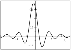
Figure 1: Graphical representation of the left hand side of Eq. (39) for k=0, a self-dual domain, and $\alpha=\pi/2$. Zeroes of the function are the radial eigenvalues $\Lambda^{--}_{0n}$.

As seen from Fig.1, in contradistinction to the eigenvalue problem in infinite volume on the space of square integrable functions the spectrum is not symmetric under reflections $\lambda\to-\lambda$. This comes from the fact that $\gamma_{5}$ does not commute with the boundary condition so that $\gamma_{5}\psi$ is not an eigenfunction if $\psi$ is an eigenfunction. An assymmetry of the spectrum is typical for the Dirac operator in odd dimensional spaces (see Des98 and references therein) and has important consequences there for the effective action. In our case the unusual boundary conditions are responsible for the assymmetry in four dimensional Euclidean space Wipf95 .

The most interesting feature of the fermionic eigenmodes becomes manifest if one considers the local chirality $X(x)$ of the lowest eigenmodes as defined by Eq. (1).

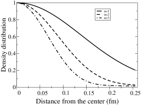
Figure 2: Normal density distribution for modes with $k=0$ and $n=1,2,3$.

IV Chirality of low lying modes

It is obvious that none of the solutions are eigenstates of $\gamma_{5}$. However at the domain center $x^{2}=0$ (or $(x-z_{j})^{2}=0$ in general) all the purely radial modes with $k=0$ have a maximum in the probability density, they are chiral and the sign of their chirality is determined by the duality of the mean field in a domain which is illustrated in Figs.2 and 3. The probability density naturally vanishes at the domain center for the modes with $k>0$ as is seen in Fig.4. To demonstrate this analytically let us turn to the local chirality parameter given in the introduction which we rewrite here in more detailed form

$$\tan\left(\frac{\pi}{4}(1-X(x))\right)=\sqrt{{\psi^{\dagger}(x)(1-\gamma_{5})\psi(x)}\over{\psi^{\dagger}(x)(1+\gamma_{5})\psi(x)}},\ -1\leq X(x)\leq 1,$$

which takes the extremal values $X=\pm 1$ at positions $x$ where $\psi(x)$ is purely right(left) handed. Because $\varphi$ and $\chi$ have the same chirality, the representation Eq.(17) immediately gives for the self-dual domain

$$\tan\left(\frac{\pi}{4}(1-X_{\rm sd}^{-\kappa}(x))\right)={{|\varphi_{00}^{-\kappa}(x)|}\over{|\chi_{00}^{-\kappa}(x)|}},$$

while for the anti-self-dual case the local chirality reads

$$\tan\left(\frac{\pi}{4}(1-X_{\rm asd}^{+\kappa}(x))\right)={{|\chi_{00}^{+\kappa}(x)|}\over{|\varphi_{00}^{+\kappa}(x)|}}.$$

Moreover due to the relation Eq.(40)

$$|\varphi_{00}^{+\kappa}(x)|=|\varphi_{00}^{-\kappa}(x)|,\ |\chi_{00}^{+\kappa}(x)|=|\chi_{00}^{-\kappa}(x)|.$$

Representations Eqs. (27) and (37) show that

$$0<\lim_{x^{2}\to 0}|\varphi_{00}^{+\kappa}(x)|<\infty,\ \lim_{x^{2}\to 0}|\chi_{00}^{+\kappa}(x)|=0,$$

which finally results in

$$X_{\rm sd}^{+\kappa}(0)=-1,\ X_{\rm asd}^{+\kappa}(0)=1.$$

The local chirality parameter $X$ as a function of distance from the domain centre for the lowest few modes is plotted in Fig.3. There is a peak in $X$ at the domain centre. Away from the centre $X$ decreases due to a competition of left and right components of the eigenmodes as the $\chi$ component becomes non-vanishing. As is seen from Fig.3 the chirality of the lowest mode ($n=1$) monotonically decreases with distance from the centre. The chirality parameter for the excited modes alternates between extremal values, the number of alternations is correlated with the radial number $n$, and the half-width decreases with growing $n$. The chirality parameter $X$ is zero at the boundary for all modes. Qualitatively this picture does not depend on the angle $\alpha$. The “width” of the peaks at half-maximum for the lowest ($n=0$) radial modes varies for different values $\alpha$ and is of the order of $0.12-0.14\ {\rm{fm}}$ if the values of $B$ and $R$ are fixed from the gluon condensate and the string tension, consistent with the lattice observations of Hor2 .

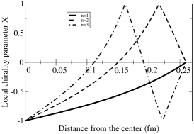
Figure 3: Chirality parameter for the three lowest radial modes $\psi_{00}^{--}$, self-dual domain, $\alpha=\pi/2$.

We can now study the chirality characteristics of the ensemble of fermion fields entering the partition function Eq.(6) with all values of $\alpha$ treated with equal probability consistent with an explicit chiral symmetry. On the lattice Hor02 ; EdH02 peaks in $X$ or $\psi^{\dagger}\psi$ would only be localiseable within a size corresponding to the lattice spacing. To take this into account, we average $X(x)$ over a small neighbourhood of the domain centre. Thus we compute the probability to find a given value of $\bar{X}$, the smeared $X$, among the chiralities for the lowest modes. The result given in Fig.5 was obtained for three sets of modes: with $n\leq 2,k=0$ (solid line), $n\leq 4,k=0$ (dashed line) and $n\leq 6,k=0$ (dot-dashed line), and all possible values of $\alpha$ and spin-colour polarizations. The solid line, formed from the lowest modes, evidently indicates two narrow peaks with $\bar{X}\approx\pm 0.87$. This double peaking is not unexpected in view of the above discussed chirality properties. Including higher modes broadens the peaks and shifts their maxima. This feature as well as the above mentioned values for the half-width and the density of domains is in qualitative and quantitative agreement with recent lattice results EdH02 ; Hor2 . It should be stressed that orbital excitations ($k>0$) are not included in the histograms. because the probability density for orbital modes vanishes at the centre. However there are maxima in the probability density for these modes in peripheral regions of the domain. The local chirality $X$ is significantly smaller in peak value than those for the radial modes at the centre. Inclusion of orbital modes will broaden the peaks more and build up the central plateau.

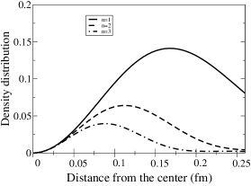
Figure 4: Plot of the radial dependence of the normal density distribution for the modes with $k=1$ and $n=1,3,5$.

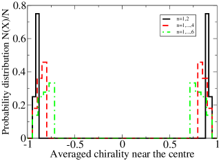
Figure 5: Histogram of chirality parameter $\bar{X}$ averaged over the central region with radius $0.025$fm. Plots given in solid, dashed and dot-dashed lines incorporate all modes with $n\leq 2$, $n\leq 4$ and $n\leq 6$ respectively.

V Discussion and conclusions

The statement that signals for spontaneous chiral symmetry breaking should be identifiable in the specific chirality properties of fermionic eigenmodes for some “dominant” gluonic background field is generally accepted. Such signals are now being seen on the lattice, but nevertheless there are not so many analytically explicit examples of this relationship available. Instanton motivated models are certainly the most advanced example of this kind. But one aspect of instanton models lies in the ‘dual’ use to which the exact fermion zero modes of the classical instanton background are subject: these modes have definite chirality and do not contribute in the infinite volume limit, but are used to model pseudo zero modes which should characterise the non-semi-classical system of strongly overlapping instantons and anti-instantons.

We have studied the spectrum of quark modes in a domainlike structured gluon background field. Such a background is argued to characterise the bulk average properties of the vacuum in the presence of strong intermediate range fluctuations and is not the result of a semi-classical approximation. The spectrum exhibits definite chirality properties. In particular, there are no zero modes because of the conditions which fermion fields must satisfy on the boundaries of domains. Nonetheless at the centre of domains all radial modes are purely chiral and the sign of their chirality depends on whether the underlying gluon field is self-dual or anti-self-dual. Moreover, the sign of chirality at the centre persists over the whole domain for the lowest modes. Studying the local chirality parameter $X$ in a chirally symmetric ensemble of domains we obtain qualitatively similar results to those seen in lattice calculations. We stress that this comparison with lattice results takes place at the level of an ensemble of configurations not on a configuration by configuration basis.

Insofar as these lattice results for chirality are argued as supporting the evidence for spontaneous chiral symmetry breaking, the same can be said of the domain model. We note the absence of any explicit zero modes in achieving this. Namely, the range of configurations needed to produce the types of effects seen on the lattice are not restricted to instanton-like fields. It suffices that a given gluon background admit strongly chiral low-lying non-zero modes. In this respect, the more significant property of the gluon background is the “locking” of chromoelectric and chromomagnetic fields into self-dual or anti-self-dual fields in relatively large but finite regions of space restricted by the hypersurfaces on which a pure gauge singularities are assumed to be situated. It should be stressed that in the thermodynamic limit the number of domains is growing but their sizes stay fixed around some finite mean value.

The solutions obtained in this paper provide a basis for computation of chiral condensate $\langle\bar{\psi}\psi\rangle$, in particular in the presence of an explicit CP violating $\theta$ term. In view of the assymmetry of the spectrum, the specific chiral properties of the eigenmodes and noninteger mean topological charge associated with a domain are expected to simultaneously enhance the role of the axial anomaly in the spontaneous breakdown of chiral flavour symmetry and factor in the solution of the $U_{\rm A}(1)$ problem Des98 ; Cre78 ; Dash71 .

Appendix A Conventions

We use a chiral representation for the antihermitian Dirac matrices in four Euclidean space,

$$\{\gamma_{\mu},\gamma_{\nu}\}=-2\delta_{\mu\nu},\ \gamma_{\mu}^{+}=-\gamma_{\mu},$$

$$\gamma_{i}=\left(\begin{array}[]{cc}0&\sigma_{i}\\ -\sigma_{i}&0\end{array}\right),\ \gamma_{4}=i\left(\begin{array}[]{cc}0&\bf{1}\\ \bf{1}&0\end{array}\right),$$

$$\gamma_{5}=\gamma_{1}\gamma_{2}\gamma_{3}\gamma_{4}={\rm diag}(1,1,-1,-1).$$

The background field is specified as

$$\hat{B}_{\mu}(x)=-\frac{1}{2}\hat{n}B_{\mu\nu}x_{\nu}$$

$$B_{ij}=\varepsilon_{ijk}B_{k},\ B_{i}=\frac{1}{2}\varepsilon_{ijk}B_{jk},\ E_{i}=B_{i4}=\pm B_{i},$$

$$B_{\mu\nu}B_{\mu\rho}=\delta_{\nu\rho}B^{2},\ \tilde{B}_{\mu\nu}=\frac{1}{2}\varepsilon_{\mu\nu\alpha\beta}B_{\alpha\beta}=\pm B_{\mu\nu},$$

In addition the following conventions and relations have been used

$$\sigma_{\mu\nu}=\frac{1}{2i}[\gamma_{\mu},\gamma_{\nu}],\ \Sigma_{i}=\frac{1}{2}\varepsilon_{ijk}\sigma_{jk},$$

$$\sigma_{ij}B_{ij}=2\Sigma_{i}B_{i},\ \Sigma_{\pm}=\frac{1}{2}\left(1\pm\frac{\Sigma_{i}B_{i}}{B}\right)$$

$$\sigma_{i4}=-\frac{1}{2}\gamma_{5}\varepsilon_{i4\mu\nu}\sigma_{\mu\nu}=-\frac{1}{2}\gamma_{5}\varepsilon_{ijk}\sigma_{jk}=-\gamma_{5}\Sigma_{i},$$

$$\gamma_{5}\sigma_{\alpha\beta}=-\tilde{\sigma}_{\alpha\beta},\ {\rm Tr}\gamma_{\mu}\gamma_{\nu}\gamma_{\alpha}\gamma_{\beta}\gamma_{5}=4\varepsilon_{\mu\nu\alpha\beta},$$

and in particular

$$\sigma_{\alpha\beta}B_{\alpha\beta} = \sigma_{ij}B_{ij}+2\sigma_{i4}B_{i4}=2\Sigma_{i}B_{i}\mp 2B_{i}\gamma_{5}\Sigma_{i}$$

$$= 4P_{\mp}\Sigma_{i}B_{i}=4BP_{\mp}(\Sigma_{+}-\Sigma_{-}).$$

We use the following hyperspherical coordinate system in $R^{4}$

$$x_{1}=r\sin\eta\cos\phi,\ x_{2}=r\sin\eta\sin\phi,$$

$$x_{3}=r\cos\eta\cos\chi,\ x_{4}=r\cos\eta\sin\chi,$$ (42)

and define the angular momentum operators as follows

$$L_{i} = -i\epsilon_{ijk}x_{j}\partial_{k},$$

$$M_{i} = -i(x_{4}\partial_{i}-x_{i}\partial_{4}),$$

respectively for spatial rotations and Euclidean “boosts”. As mentioned, it is more convenient to work in the basis

$${\bf K}_{1,2}=({\bf L}\pm{\bf M})/2$$

which generates the following Lie algebra

$$\left[K_{1}^{i},K_{1}^{j}\right]=i\epsilon^{ijk}K_{1}^{k},\ \left[K_{2}^{i},K_{2}^{j}\right]=i\epsilon^{ijk}K_{2}^{k},\ \left[K_{1}^{i},K_{2}^{j}\right]=0.$$

Thus the ladder operators

$$K_{1,2}^{\pm}=(K_{1,2}^{1}\pm iK_{1,2}^{2}),$$

satisfy the algebra

$$\left[K_{1,2}^{3},K_{1,2}^{\pm}\right]=\pm K_{1,2}^{\pm}$$

and correspond to raising and lowering operators of $m_{1},m_{2}$.

The angular eigenfunctions corresponding to the ${\bf K}_{1,2}$ generators are

$$C_{km_{1}m_{2}}(\eta,\phi,\chi) = (-1)^{|m_{1}+m_{2}|}(2\pi)^{-1}\Theta_{k}^{m_{1}-m_{2},m_{1}+m_{2}}(\eta),$$

$$\times \exp i[(m_{1}-m_{2})\chi+(m_{1}+m_{2})\phi]$$

$$\Theta_{k}^{k-r-s,s-r}(\eta) = \sqrt{2(k+1)(k-r)!(k-s)!r!s!}$$

$$\times \sum_{n=0}^{r}{{(-1)^{r-n}\cos^{k-r-s+2n}\eta\sin^{r+s-2n}\eta}\over{(k-r-s+n)!n!(r-n)!(s-n)!}},$$

$$s=(k+m_{2})/2,\ r=(k-m_{1})/2,$$

where $k,m_{1},m_{2}$ are respectively the orbital angular momentum and the two azimuthal quantum numbers, relevant for an $O(4)=O(3)\times O(3)$ symmetry. They take the following values

$$k=0,1,2,\dots,\ m_{1},m_{2}=-\frac{k}{2},\dots,\frac{k}{2}.$$

Appendix B Dirac eigenvalue problem in a domain.

Here we give further details of the solution of Eq.(I). Using the notation given in the main body, we can decompose the field $\varphi$ over a set of chiral and colour-spin projectors

$$\varphi=P_{\pm}\Phi_{0}+P_{\mp}O_{+}\Phi_{+1}+P_{\mp}O_{-}\Phi_{-1},$$

where (lower)upper signs correspond to the (anti-)self-dual field background field, and fields $\Phi_{\zeta}$ must satisfy the second order equation

$$(-D^{2}+2\zeta\hat{B}-\lambda^{2})P_{\mp}O_{\zeta}\Phi_{\zeta}=0.$$ (43)

We remind that implicitly $\Phi_{\zeta}^{\alpha}$ is the color vector in the fundamental representation.

If we were solving the problem for square integrable eigenfunctions in infinite volume then all three components $\Phi_{\zeta}$ would enter the final set of eigenfunctions, moreover as is seen from Eq.(43), the equation for the component $\Phi_{-1}$ would produce zero modes with chirality $\mp 1$. The spectrum in this case would be discrete and all nonzero eigenvalues of Dirac operator come in pairs: if $\psi$ is an eigen function with eigenvalue $\lambda$ then $\gamma_{5}\psi$ is an eigenfunction with eigen value $-\lambda$ – pretty standard state of affairs.

However the bag-like boundary conditions Eq.(8) we must satisfy in the present case change the structure of eigenfunctions and eigenvalues drastically. First of all, because of the identities

$$\gamma_{\mu}B_{\mu\rho}x_{\rho}P_{\mp}\Sigma_{+}=iB\!\not\!xP_{\mp}\Sigma_{+},$$

$$\gamma_{\mu}B_{\mu\rho}x_{\rho}P_{\mp}\Sigma_{-}=-iB\!\not\!xP_{\mp}\Sigma_{-}.$$

and

$$\gamma_{\mu}B_{\mu\rho}x_{\rho}P_{\pm}\Sigma_{+}=\left\{\frac{2i}{x^{2}}B[x_{i}^{2}-(B_{i}x_{i})^{2}/B^{2}]-iB\right\}\!\not\!xP_{\pm}\Sigma_{+}$$

$$\gamma_{\mu}B_{\mu\rho}x_{\rho}P_{\pm}\Sigma_{-}=-\left\{\frac{2i}{x^{2}}B[x_{i}^{2}-(B_{i}x_{i})^{2}/B^{2}]-iB\right\}\!\not\!xP_{\pm}\Sigma_{-},$$

which can be straightforwardly derived by expanding both sides over a complete set of Dirac matrices, the bag-like boundary condition can be satisfied only for the trivial solution $\Phi_{0}(x)\equiv 0$. The significance of this observation is that for (anti-)self-dual domains the boundary condition can only be implemented on eigenspinors $\psi=i\!\not\!\eta\chi+\phi$ for (positive) negative chirality $\varphi$ and $\chi$. The function $\psi$ in turn is not an eigenspinor of $\gamma_{5}$, which is natural because the boundary condition violates chiral symmetry. Furthermore, zero modes are removed from the spectrum because they must be chiral but this is forbidden by boundary conditions. And, finally, if $\psi$ is an eigenfunction with eigenvalue $\lambda$ then $\gamma_{5}\psi$ is not an eigenfunction any more, and there is no eigenvalue $-\lambda$ in the spectrum.

In order to find equations for components $\Phi^{\alpha}_{\zeta}$ of the corresponding spinors we use that

$$\varphi_{-\pm}=P_{-}O_{\pm}\Phi_{\pm 1}=\left(0,0,N_{\mp}\Phi^{3}_{\pm 1},N_{\pm}\Phi^{4}_{\pm 1}\right)^{\rm T},$$

$$\varphi_{+\pm}=P_{+}O_{\pm}\Phi_{\pm 1}=\left(N_{\mp}\Phi^{1}_{\pm 1},N_{\pm}\Phi^{2}_{\pm 1},0,0\right)^{\rm T}.$$ (44)

In hyperspherical coordinates Eqs.(42) the equations for the spinor components read (here and below we write down equations for the self-dual case only)

$$\left\{-\left[\frac{1}{r^{3}}\partial_{r}r^{3}\partial_{r}-\frac{4}{r^{2}}{\bf K}_{1}^{2}+2\frac{\hat{n}}{|\hat{n}|}\hat{B}K_{2z}-\frac{1}{4}\hat{B}^{2}r^{2}\right]+2\hat{B}-\lambda^{2}\right\}N_{-}\Phi_{+1}^{3}=0,$$

$$\left\{-\left[\frac{1}{r^{3}}\partial_{r}r^{3}\partial_{r}-{\frac{4}{r^{2}}}{\bf K}_{1}^{2}+2\frac{\hat{n}}{|\hat{n}|}\hat{B}K_{2z}-\frac{1}{4}\hat{B}^{2}r^{2}\right]+2\hat{B}-\lambda^{2}\right\}N_{+}\Phi_{+1}^{4}=0,$$

$$\left\{-\left[\frac{1}{r^{3}}\partial_{r}r^{3}\partial_{r}-\frac{4}{r^{2}}{\bf K}_{1}^{2}+2\frac{\hat{n}}{|\hat{n}|}\hat{B}K_{2z}-\frac{1}{4}\hat{B}^{2}r^{2}\right]-2\hat{B}-\lambda^{2}\right\}N_{+}\Phi_{-1}^{3}=0,$$

$$\left\{-\left[\frac{1}{r^{3}}\partial_{r}r^{3}\partial_{r}-\frac{4}{r^{2}}{\bf K}_{1}^{2}+2\frac{\hat{n}}{|\hat{n}|}\hat{B}K_{2z}-\frac{1}{4}\hat{B}^{2}r^{2}\right]-2\hat{B}-\lambda^{2}\right\}N_{-}\Phi_{-1}^{4}=0,$$ (45)

The anti-self-dual case is reconstructed by the change $K_{2z}\to K_{1z}$ and $\Phi_{\zeta}^{3}\to\Phi_{\zeta}^{1}$, $\Phi_{\zeta}^{4}\to\Phi_{\zeta}^{2}$. In KaNe01 we derived the general solution for equations of this type. The requirement of regularity at the origin then gives

$$\Phi_{+1}^{3,km_{1}m_{2}} = N_{-}z^{k/2}e^{-z/2}M\left(\frac{k}{2}+m_{2}-\Lambda^{2}+2,k+2,z\right){\cal C}_{km_{1}m_{2}}(\varphi,\chi,\eta),$$

$$\Phi_{+1}^{4,km_{1}m_{2}} = N_{+}z^{k/2}e^{-z/2}M\left(\frac{k}{2}-m_{2}-\Lambda^{2}+2,k+2,z\right){\cal C}_{km_{1}m_{2}}(\varphi,\chi,\eta),$$

$$\Phi_{-1}^{3,km_{1}m_{2}} = N_{+}z^{k/2}e^{-z/2}M\left(\frac{k}{2}-m_{2}-\Lambda^{2},k+2,z\right){\cal C}_{km_{1}m_{2}}(\varphi,\chi,\eta),$$

$$\Phi_{-1}^{4,km_{1}m_{2}} = N_{-}z^{k/2}e^{-z/2}M\left(\frac{k}{2}+m_{2}-\Lambda^{2},k+2,z\right){\cal C}_{km_{1}m_{2}}(\varphi,\chi,\eta),$$

where $\Lambda=\lambda/\sqrt{2\hat{B}}$, $z=\hat{B}r^{2}/2$. Thus the two independent mutually orthogonal solutions are

$$\varphi^{-+} = \left(\begin{array}[]{c}0\\ 0\\ N_{-}z^{k/2}e^{-z/2}M\left(\frac{k}{2}+m_{2}-\Lambda^{2}+2,k+2,z\right){\cal C}_{km_{1}m_{2}}\\ N_{+}z^{k^{\prime}/2}e^{-z/2}M\left(\frac{k^{\prime}}{2}-m^{\prime}_{2}-\Lambda^{\prime 2}+2,k^{\prime}+2,z\right){\cal C}_{k^{\prime}m^{\prime}_{1}m^{\prime}_{2}}\end{array}\right),$$ (50)

$$\varphi^{--} = \left(\begin{array}[]{c}0\\ 0\\ N_{+}z^{k/2}e^{-z/2}M\left(\frac{k}{2}-m_{2}-\Lambda^{2},k+2,z\right){\cal C}_{km_{1}m_{2}}\\ N_{-}z^{k^{\prime}/2}e^{-z/2}M\left(\frac{k^{\prime}}{2}+m^{\prime}_{2}-\Lambda^{\prime 2},k^{\prime}+2,z\right){\cal C}_{k^{\prime}m^{\prime}_{1}m^{\prime}_{2}}\end{array}\right),$$ (55)

where “prime” indicates that angular quantum numbers and eigenvalues in the third line need not coincide with those in the fourth in order that these spinors be eigenmodes of Eq.(14).

To obtain an explicit representation for $\chi$ we use the identity:

$$-\!\not\!\eta(x)\!\not\!D=\partial_{r}+2R^{-1}({\bf\Sigma}\cdot{\bf K}_{1}P_{+}+{\bf\Sigma}\cdot{\bf K}_{2}P_{-})-i\!\not\!\eta\frac{\hat{n}}{2}\gamma_{\mu}B_{\mu\nu}x_{\nu},$$ (56)

where the action of the last term on $P_{\mp}O_{\zeta}\Phi^{\zeta}$ can be determined via the identity

$$\frac{\hat{n}}{2}\gamma_{\mu}B_{\mu\nu}x_{\nu}P_{\mp}O_{\zeta}=i\zeta\!\not\!\eta\frac{\hat{B}R}{2}P_{\mp}O_{\zeta},$$

and the action of the ${\bf\Sigma}\cdot{\bf K}$ terms via

$${\bf\Sigma}\cdot{\bf K}_{1,2}\sum_{\zeta}O_{\zeta}\Phi_{\zeta} = \left(\Sigma_{3}K^{z}_{1,2}+\Sigma^{(+)}K^{-}_{1,2}+\Sigma^{(-)}K^{+}_{1,2})\right)\sum_{\zeta}O_{\zeta}\Phi_{\zeta}$$ (57)

$$= \frac{\hat{n}}{|\hat{n}|}K^{z}_{1,2}\left(O_{+}\Phi_{+1}-O_{-}\Phi_{-1}\right)$$

$$+N_{+}\Sigma^{(+)}K^{-}_{1,2}\Phi_{+1}+N_{-}\Sigma^{(+)}K^{-}_{1,2}\Phi_{-1}+N_{-}\Sigma^{(-)}K^{+}_{1,2}\Phi_{+1}+N_{+}\Sigma^{(-)}K^{+}_{1,2}\Phi_{-1}.$$

As well as the ladder operators $K^{\pm}$ we also have analogous operators for the spin,

$$\Sigma^{(\pm)}=\frac{1}{2}(\Sigma_{1}\pm i\Sigma_{2}).$$

For $B_{i}=B\delta_{i3}$ the following identities are also useful for implementing the above

$$\Sigma_{3}O_{\pm}=\pm\frac{\hat{n}}{|\hat{n}|}O_{\pm},\ \Sigma^{(+)}O_{\pm}=N_{\pm}\Sigma^{(+)},\ \Sigma^{(-)}O_{\pm}=N_{\mp}\Sigma^{(-)},$$

and

$$P_{-}\Sigma^{(+)}\Psi = \left(0,0,-\Psi^{4},0\right)^{\rm T},$$

$$P_{-}\Sigma^{(-)}\Psi = \left(0,0,0,-\Psi^{3}\right)^{\rm T},$$

$$P_{+}\Sigma^{(+)}\Psi = \left(-\Psi^{2},0,0,0\right)^{\rm T},$$

$$P_{+}\Sigma^{(-)}\Psi = \left(0,-\Psi^{1},0,0\right)^{\rm T}.$$ (58)

We thus get for the self-dual case

$$\chi^{-+} = \left(\begin{array}[]{c}0\\ 0\\ \frac{1}{i\lambda}[\partial_{r}-\frac{\hat{B}r}{2}-\frac{2}{r}K_{2}^{3}]N_{-}z^{k/2}e^{-z/2}M\left(\frac{k}{2}+m_{2}-\Lambda^{2}+2,k+2,z\right){\cal C}_{km_{1}m_{2}}\\ \frac{1}{i\lambda^{\prime}}[\partial_{r}-\frac{\hat{B}r}{2}+\frac{2}{r}K_{2}^{3}]N_{+}z^{k^{\prime}/2}e^{-z/2}M\left(\frac{k^{\prime}}{2}-m^{\prime}_{2}-\Lambda^{\prime 2}+2,k^{\prime}+2,z\right){\cal C}_{k^{\prime}m^{\prime}_{1}m^{\prime}_{2}}\end{array}\right)$$ (63)

$$- \frac{2}{r}\left(\begin{array}[]{c}0\\ 0\\ \frac{1}{i\lambda^{\prime}}K_{2}^{-}N_{+}z^{k^{\prime}/2}e^{-z/2}M\left(\frac{k^{\prime}}{2}-m^{\prime}_{2}-\Lambda^{\prime 2}+2,k^{\prime}+2,z\right){\cal C}_{k^{\prime}m^{\prime}_{1}m^{\prime}_{2}}\\ \frac{1}{i\lambda}K_{2}^{+}N_{-}z^{k/2}e^{-z/2}M\left(\frac{k}{2}+m_{2}-\Lambda^{2}+2,k+2,z\right){\cal C}_{km_{1}m_{2}}\end{array}\right)$$ (68)

and

$$\chi^{--} = \left(\begin{array}[]{c}0\\ 0\\ \frac{1}{i\lambda}[\partial_{r}+\frac{\hat{B}r}{2}-\frac{2}{r}K_{2}^{3}]N_{+}z^{k/2}e^{-z/2}M\left(\frac{k}{2}-m_{2}-\Lambda^{2},k+2,z\right){\cal C}_{km_{1}m_{2}}\\ \frac{1}{i\lambda^{\prime}}[\partial_{r}+\frac{\hat{B}r}{2}+\frac{2}{r}K_{2}^{3}]N_{-}z^{k^{\prime}/2}e^{-z/2}M\left(\frac{k^{\prime}}{2}+m^{\prime}_{2}-\Lambda^{\prime 2},k^{\prime}+2,z\right){\cal C}_{k^{\prime}m^{\prime}_{1}m^{\prime}_{2}}\end{array}\right)$$ (73)

$$- \frac{2}{r}\left(\begin{array}[]{c}0\\ 0\\ \frac{1}{i\lambda^{\prime}}K_{2}^{-}N_{-}z^{k^{\prime}/2}e^{-z/2}M\left(\frac{k^{\prime}}{2}+m^{\prime}_{2}-\Lambda^{\prime 2},k^{\prime}+2,z\right){\cal C}_{k^{\prime}m^{\prime}_{1}m^{\prime}_{2}}\\ \frac{1}{i\lambda}K_{2}^{+}N_{+}z^{k/2}e^{-z/2}M\left(\frac{k}{2}-m_{2}-\Lambda^{2},k+2,z\right){\cal C}_{km_{1}m_{2}}\end{array}\right).$$ (78)

By inspection, the boundary condition $\chi=-e^{-i\alpha}\varphi$ can only be fulfilled if terms with raising/lowering operators of the azimuthal quantum numbers vanish since these terms contain the projectors $N_{\pm}$ while the rest of terms entering the boundary condition contain $N_{\mp}$ (see Eqs. (50) and (55)). In particular, $m^{\prime}_{2}=-k/2,\ m_{2}=k/2$. Finally, evaluating the derivatives of the confluent hypergeometric functions with the help of relation

$$M^{\prime}_{z}(a,b,z)=\frac{a}{b}M(a+1,b+1,z)$$

leads to the solutions given in the main body of the paper.

References

• (1) A.C. Kalloniatis, S. N. Nedelko, Phys.Rev. D 64, 114025 (2001).
• (2) Some selected references are: M.J. Teper, Phys. Lett. B162, 357 (1985); E.-M. Ilgenfritz et al., Nucl. Phys. B268, 693 (1986); M.J. Teper, Nucl. Phys. B (Proc. Suppl.) 83, 146 (2000); UKQCD Collaboration, Douglas A. Smith et al., Phys. Rev. D 58, 014505 (1998); Philippe de Forcrand et al., Nucl. Phys. B (Proc. Suppl.) 63, 549 (1998) see also hep-lat/9802017. For a relationship between cooling and smearing see F. Bonnet et al., Phys. Rev. D 62, 094509 (2000); hep-lat/0106023.
• (3) T.L. Ivanenko and J.W. Negele, Nucl. Phys. B (Proc. Suppl.) 63, 504 (1998); R.G. Edwards, U.M. Heller, and R. Narayanan, Nucl. Phys. B522, 285 (1998).
• (4) J.B. Zhang, S.O. Bilson-Thompson, F.D.R. Bonnet, D.B. Leinweber,A.G. Williams, J.M. Zanotti, Phys.Rev.D 65, 074510 (2002).
• (5) Robert G. Edwards, Urs M. Heller, Phys.Rev. D 65, 014505 (2002).
• (6) T. Banks, A. Casher, Nucl.Phys.B167, 215 (1980).
• (7) I.Horvath, N. Isgur, J.McCune, H.B. Thacker, Phys.Rev. D 65, 014502 (2002).
• (8) N. Cundy, M. Teper, U. Wenger, hep-lat/0203030.
• (9) R.G. Edwards, Nucl.Phys. B (Proc.Suppl.) 106, 38 (2002).
• (10) T. DeGrand, Phys.Rev. D 64, 094508 (2001).
• (11) O. Jahn, F. Lenz, Phys. Rev. D 58, 085006 (1998); F. Lenz, S. Worlen, At the frontier of particle physics, vol. 2, 683-760, ed. by M. Shifman, World Scientific, 2001 (hep-ph/0010099).
• (12) P. van Baal, At the frontier of particle physics, vol. 2, 760-821, ed. by M. Shifman, World Scientific, 2001 (hep-ph/0008206).
• (13) C. Ford et al, Ann. Phys. (N.Y.) 269, 26 (1998).
• (14) P. Di Vecchia, G. Veneziano, Nucl.Phys.B171, 253 (1980); E. Witten, Annals Phys.128, 363 (1980).
• (15) A. Wipf and S. Duerr, Nucl. Phys. B443, 201 (1985).
• (16) S. Deser et al., Phys. Rev. D 57, 7444 (1998).
• (17) I. Horvath et al. hep-lat/0201008.
• (18) R.J. Crewther, “Chiral Properties of Quantum Chromodynamics”, Kaiserslautern NATO Inst.1979:0529 (QCD161:N16:1979); Nucl.Phys. B209, 413 (1982). See also, R.J. Crewther, Phys.Lett.B70, 349 (1977).
• (19) R. Dashen, Phys. Rev. D 3, 1879 (1971).