On Nonstandard Vacuua in Minimal Supergravity Models.

Abstract:

The plethora of scalar fields participating in the formulation of a softly broken supersymmetric theory can threat the stability of the standard vacuum. The generic situation is twofold. Directions in scalar field space may exist along which the potential becomes unbounded from below or local minima deeper than the standard one are likely to appear where charge and/or color symmetries are broken. An investigation of these matters requires a thorough study of the tree level effective potential as well as its radiative corrections. However, the presence of many different mass scales in such a generic supersymmetric theory needs an appropriate renormalization improved treatment. Combining the decoupling theorem with a conveniently chosen renormalization scale for each field configuration, the well known multimass scale problem is circumvented. In this context, the ordinary universal soft-parameters case of the minimal supersymmetric model as well as a non-universal case of a brane world minimal supergravity model are examined closely for unphysical vacuua.

1 Introduction

Supersymmetric (SUSY) theories are the best motivated extensions of the Standard Model (SM) of the electroweak and strong interactions. They provide an elegant way to stabilize the huge hierarchy between the Grand Unification (GUT) and the Fermi scale, and predict a variety of new matter states (sparticles) creating a natural framework to cancel the quadratic divergences of the radiative corrections to the Higgs boson mass. One can classify these models by the mechanism for communicating SUSY breaking from a hidden sector to the observable sector. Possibilities include gravity mediated SUSY breaking (SUGRA) [1], gauge mediated SUSY breaking, [2] and anomaly mediated SUSY breaking [3].

The so-called minimal supergravity (mSUGRA) model has traditionally been the most popular choice for phenomenological SUSY analyses. In mSUGRA, it is assumed that its most economical low energy realization, the so called Minimal Supersymmetric Standard Model (MSSM) [4], is valid from the weak scale all the way up to the GUT scale $M_{X}\simeq 2\times 10^{16}$ GeV, where this choice is usually taken due to apparent gauge coupling unification. In the MSSM one assumes a minimal gauge group, i.e. ${\rm SU(3)_{C}}\times{\rm SU(2)_{L}}\times{\rm U(1)_{Y}}$, and a minimal particle content, i.e. three generations of fermions (no right handed neutrinos included) and their spin zero partners as well as two Higgs doublet superfields to break the electroweak symmetry. In order to explicitly break supersymmetry while preventing the reappearance of quadratic divergences, a collection of soft terms [5] is added to the Lagrangian: mass terms for the gauginos ($m_{1/2}$), mass terms for the scalar fermions ($m_{0}$), mass and bilinear terms for the Higgs bosons ($B_{0}$), and trilinear couplings ($A_{0}$) between sfermions and Higgs bosons. In the general case, that is if one allows for intergenerational mixing and complex phases, the soft SUSY breaking terms will introduce a huge number of unknown parameters. This feature makes any phenomenological analysis in the general MSSM a daunting task. In this context, severe phenomenological constraints are imposed on the parameter space by flavor changing neutral currents (FCNC) and CP violation [6] as well as unphysical vacuua.

To reduce the number of free parameters, one needs an explanation of how supersymmetry is broken. In mSUGRA, supersymmetry is spontaneously broken via a hidden sector field vacuum expectation value (VEV), and the SUSY breaking is communicated to the visible sector via gravitational interactions. For a flat Kähler metric $G_{i}^{j}$ and common gauge kinetic functions $f_{AB}$, this leads to universal values for $m_{0}$, $m_{1/2}$ and $A_{0}$, $B_{0}$ at the GUT scale $M_{X}$. This assumption of universality in the scalar sector leads to the phenomenologically required suppression of flavor violating processes that are supersymmetric in origin. However, there is no known physical principle which gives rise to the desired form of $G_{i}^{j}$ and $f_{AB}$; indeed, for general forms of $G_{i}^{j}$ and $f_{AB}$, non-universal masses are expected. Hence, the universality assumption is regarded as being entirely motivated by the phenomenological need for suppression of flavor violating processes in the MSSM.

In recent years the branes, which are typical in models with extra dimensions [7], have been found to fit naturally with the idea of breaking supersymmetry via a hidden sector. The basic five-dimensional setup of brane world models [8] is that of four-dimensional hypersurfaces (branes) hosting familiar gauge and matter fields, which are embedded in a higher dimensional ambient space, the bulk, populated by gravitational and gauge-neutral fields. The bulk degrees of freedom couple to the fields living on branes through various types of interactions, but the effects of SUSY-breaking will be communicated gravitationally to the observable world through the five-dimensional interior bulk. This scenario thereby places the question of SUSY-breaking in an entirely new geometric context.

Brane world SUSY breaking generally gives rise to tree-level soft scalar masses for visible sector squark and slepton fields. These masses are generally not universal. Without additional assumptions about flavor, these non-universal scalar mass matrices are not necessarily aligned with the quark and lepton mass matrices, and dangerous sflavor violation can occur. A model to overcome this flavor problem has been recently proposed. The authors of Ref. [9] have suggested a gravity mediated SUSY breaking in 5D spacetime with two 4D branes B1 and B2 separated in the extra dimension. The SUSY breaking effects from the hidden sectors localized on the branes are transmitted through gravitational couplings both to the visible sector fields located on the same brane and to bulk gauginos. Thus, if the SUSY breaking scales are $m_{1}$ and $m_{2}$ at two separated branes B1 and B2 respectively, the localized chiral multiplets at B1 (B2) could get soft SUSY breaking effects of order $m_{1}$ ($m_{2}$). Assuming that the SUSY breaking scales at B1 and B2 are $m_{1}$ ($\sim$ 10–20 TeV) $>$ $m_{2}$ ($\sim$ 1 TeV), the superpartners of the first two generations can be easily made sufficiently heavy to overcome the SUSY flavor problem by locating them on B1. In order to keep the radiative corrections to the Higgs masses under control, the third family must reside on B2. The two Higgs multiplets should reside in the bulk, so that the first two and the third generations of the quarks and leptons can couple to them at B1 and B2, respectively.

Beyond the SUSY flavor requirements, an additional constraint on mSUGRA parameters can be obtained by demanding that the global minimum of the scalar potential is indeed the minimum that leads to appropriate electroweak symmetry breaking [10]. From a theoretical point of view, the plethora of new scalar fields which are introduced in MSSM may lead to many possible directions in field space where field configurations could be developed deeper than the standard minimum. The generic situation [11, 12, 13, 14, 15] is that the scalar potential can receive negative contributions from quadratic or cubic term in the supersymmetry breaking Lagrangian if the usually dominated quartic $D$ and $F$ terms are suppressed. A systematic classification of all possible dangerous directions in the scalar field space that can potentially lead to undesirable minima has been done by the authors of Ref. [12]. These directions have been categorized either as field directions that are unbounded from below (UFB) or as directions that lead to charge or color breaking minima (CCB).

The purpose of this work is to extend and complement the work done on this subject by analyzing the impacts the one loop radiative corrections have on these unphysical configurations for the models described above. Yet, the effective potential in which the vacuum structure is encoded, is a poorly known object beyond the tree-level approximation. One reason for this is the dependence of its loop corrections upon the very many different mass scales present in these models, so that a renormalization group analysis becomes rather tricky. In general, when one deals with a system possessing a large mass scale $Q_{M}$, compared with the scale $Q_{\mu}$ at which one discusses physics, large logarithms such as $\ln(Q_{M}/Q_{\mu})$ always appear which affect the convergence of the loop expansion. In this situation, one considers resuming the perturbation series by using the renormalization group equation (RGE). Nonetheless, in many realistic applications one often has to deal with an additional mass scale $Q_{m}$ with the hierarchy $Q_{\mu}\ll Q_{m}\ll Q_{M}$. For instance, one can regard $Q_{\mu},Q_{m},Q_{M}$ as the weak, supersymmetry-breaking and unification scales respectively. When we study such a system, we face the problem of multimass scales [16]: There appear several types of logarithms $\ln(Q_{M}/Q_{\mu})$ and $\ln(Q_{m}/Q_{\mu})$, while we are able to sum up just a single logarithm by means of the RGE.

In the present work, trying to circumvent this problem, a generalized improving procedure based on Refs [17, 18] is applied to the relevant effective potential. The main idea of the method is to make use of the decoupling theorem [19] combined with a conveniently chosen renormalization scale $Q^{*}$ for each field configuration. By this procedure, it is made possible to treat essentially a single log factor at any renormalization scale, since all the heavy particles (heavier than that scale) decouple and all the light particles (lighter than that scale) yield more or less the same log factors.

The rest of this paper is organized as follows. After setting our notation and conventions in Sec. 2, an estimation of the physical vacuum is attempted in various effective low energy SUSY models in Sec. 3. Next, section 4 describes briefly the most dangerous directions that could lead to unphysical situations and Sec. 5 is an outline of our calculational scheme. In Sec. 6 we give a brief summary of our results and section 7 summarizes our conclusions. Finally, detailed formulae for the various mass matrix elements involved in one loop expressions of the effective potential are presented in Appendices.

2 The Physical Set-up

Let us briefly review some of the basic ingredients required for our analysis. A globally supersymmetric and $SU(3)_{C}\otimes SU(2)_{L}\otimes U(1)_{Y}$ gauge invariant Lagrangian with minimal content can be constructed from the usual $R$-symmetry conserving superpotential

$$\mathcal{W}=\mbox{\boldmath$Y_{e}$}{\hat{L}}^{j}{\hat{E}}^{c}{\hat{\cal H}}_{1}^{i}\epsilon_{ij}+\mbox{\boldmath$Y_{d}$}{\hat{Q}}^{ja}{\hat{D}}_{a}^{c}{\hat{\cal H}}_{1}^{i}\epsilon_{ij}+\mbox{\boldmath$Y_{u}$}{\hat{Q}}^{ja}{\hat{U}}_{a}^{c}{\hat{\cal H}}_{2}^{i}\epsilon_{ij}+\mu{\hat{\cal H}}_{1}^{i}{\hat{\cal H}}_{2}^{j}\epsilon_{ij}$$ (1)

where ${\hat{Q}}^{T}=(\hat{u}~{}~{}\hat{d})$, ${\hat{U}}^{c}$, ${\hat{D}}^{c}$ are the Quark Superfields, ${\hat{L}}^{T}=(\hat{\nu}~{}~{}\hat{\ell})$, ${\hat{E}}^{c}$ are the Lepton Superfields and ${\hat{\cal H}}^{T}_{1}=(\hat{H}_{1}~{}~{}\hat{h}_{1})$, ${\hat{\cal H}}^{T}_{2}=(\hat{h}_{2}~{}~{}\hat{H}_{2})$ are the Higgs Superfields. Generally the Yukawa matrices $Y_{u}$, $Y_{d}$, $Y_{e}$ and the parameter $\mu$ are complex.

In order to explicitly break supersymmetry as required by experiment, while keeping quadratic divergences suppressed, a collection of soft terms is added to the Lagrangian. These include: mass terms for all scalar fermions and gauginos, bilinear terms for the Higgs bosons and trilinear interactions between sfermions and Higgses. Consequently, the most general soft SUSY breaking Lagrangian with real mass terms in this minimal scheme is

$$\mathcal{L}_{SOFT} = -\frac{1}{2}M_{1}(\tilde{B}\tilde{B})-\frac{1}{2}M_{2}(\tilde{W^{\Gamma}}\tilde{W^{\Gamma}})-\frac{1}{2}M_{3}(\tilde{G^{R}}\tilde{G^{R}})$$ (2)

$$-m_{H_{1}}^{2}|{\cal H}_{1}|^{2}-m_{H_{2}}^{2}|{\cal H}_{2}|^{2}-m^{2}_{\tilde{Q}}|\tilde{Q}|^{2}-m^{2}_{\tilde{D}^{c}}|\tilde{D}^{c}|^{2}-m^{2}_{\tilde{U}^{c}}|\tilde{U}^{c}|^{2}$$

$$-m^{2}_{\tilde{L}}|\tilde{L}|^{2}-m^{2}_{\tilde{E}^{c}}|\tilde{E}^{c}|^{2}-(\mbox{\boldmath$h_{e}$}\tilde{L}^{j}\tilde{E}^{c}{\cal H}_{1}^{i}\epsilon_{ij}+\mbox{\boldmath$h_{d}$}\tilde{Q}^{ja}\tilde{D}_{a}^{c}{\cal H}_{1}^{i}\epsilon_{ij}$$

$$+\mbox{\boldmath$h_{u}$}\tilde{Q}^{ja}\tilde{U}_{a}^{c}{\cal H}_{2}^{i}\epsilon_{ij}+\mbox{H.c.})-(B\mu{\cal H}_{1}^{i}{\cal H}_{2}^{j}\epsilon_{ij}+\mbox{H.c.})$$

Here ${\cal H}_{1}$, ${\cal H}_{2}$ are the ordinary Higgs boson doublets, $\tilde{Q}$, $\tilde{D}^{c}$, $\tilde{U}^{c}$, $\tilde{L}$, $\tilde{E}^{c}$ are the squark-slepton scalar fields and $\mbox{\boldmath$h$}\equiv\mbox{\boldmath$Y$}\mbox{\boldmath$A$}$, where $A$ is a $3\times 3$ matrix containing the “soft” trilinear scalar couplings. All extra soft parameters except masses are generally complex.

Altogether one would then need more than 100 real parameters to describe SUSY breaking in full generality. Clearly, some simplifying assumptions are necessary if we want to make comprehensive scans in parameter space. Specifically, we shall work with real and diagonal Yukawa couplings where all non-zero entries are positive. Also $\mu$, $B$ and all trilinear soft couplings $A$ are assumed to be real. In our analysis we shall also keep Yukawas and trilinear soft couplings from light families, since their contributions to the one-loop effective potential (our main objective) are not always negligible for an arbitrary field configuration. For clarity reasons, we simplify the notation using $Y_{u}^{1}=Y_{u},~{}Y_{u}^{3}=Y_{t},~{}Y_{e}^{1}=Y_{e},~{}Y_{d}^{3}=Y_{b}$ and similarly for the trilinear couplings.

A dramatic decrease of the unknown parameters arises when the minimal model just presented is embedded into various supergravity scenarios. The simplest case of the MSSM results from coupling with $N=1$ Supergravity. This leads to the following “universal” scenario at a very large scale $M_{X}\simeq 2\times 10^{16}$ GeV with: $(1)$ Common gaugino mass : $m_{1/2}$, $(2)$ Common scalar mass : $m_{0}$, $(3)$ Common trilinear scalar coupling : $A_{0}$. This reduces the number of free parameters describing SUSY breaking to just four : The gaugino mass $m_{1/2}$, the scalar mass $m_{0}$, the trilinear and bilinear soft breaking parameters $A_{0}$ and $B$, which is conventionally trade with the Higgs VEV ratio $\tan\beta=\langle H_{2}^{0}\rangle/\langle H_{1}^{0}\rangle$. We also assume unification of the gauge couplings at the scale $M_{X}$, while no specific relation is assumed for the Yukawa couplings there.

However, more complicated alternatives also exist which give definite predictions for scalar, gaugino masses and soft trilinear terms appearing in Eq. (2). As we have mentioned in the introduction, one such possibility is the recently proposed 5D supergravity model of Ref. [9]. In this model the chiral matter content resides on two 4D branes separated in the extra dimension. Higgs bosons as well as gravity and gauge multiplets reside in the bulk. It is then shown that the SUSY breaking effects from the hidden sectors localized on the branes are transmitted to the visible sector fields located on the same brane and bulk gauginos through gravitational couplings. Trying to overcome the SUSY flavor problem, two SUSY breaking scales $m_{1},m_{2}$ are introduced at the separated branes $B_{1}$ and $B_{2}$, respectively. Then the localized chiral multiplets at $B_{1}(B_{2})$ could get soft SUSY breaking effects of order $m_{1}(m_{2})$. Assuming that the first two generations reside at $B_{1}$ and the third one is at $B_{2}$, the following non universal soft terms are derived

$$m_{0,i}^{2} = \frac{8m_{1}^{2}}{9}(\delta_{i1}+\delta_{i2})+\frac{8m_{2}^{2}}{9}\delta_{i3}$$ (3)

$$A_{0,i} = \frac{4m_{1}}{3}(\delta_{i1}+\delta_{i2})+\frac{4m_{2}}{3}\delta_{i3}$$ (4)

where $i$ runs on three generations. Mass terms for the gauginos can be generated at tree level in a $D=5$ off-shell SUGRA formalism [20]. If SUSY is spontaneously broken at brane $B_{1}$, heavy gaugino masses given by $m_{1/2}\simeq m_{1}\,(M_{*}/M_{P})$, where $M_{*}$ is a 5D SUGRA fundamental scale and $M_{P}$ is the reduced 4D Planck scale, could give rise to large radiative corrections to the Higgs mass and spoil the naturalness solution. However, a not so “large” extra dimension, for example of the order of $L^{-1}\sim 10^{16}$ GeV (or $M_{*}\simeq 10L^{-1}\sim 10^{17}$ GeV) suppresses the gaugino masses to 1 TeV scale. Note that the cutoff scale $\Lambda_{c}$ introduced to obtain an effective 4D theory from the 5D one, is of the order of the extra dimension. Hence, the effective theory below $\Lambda_{c}\sim M_{X}$ resembles the familiar gravity mediated scenario of MSSM.

In order to discuss the physical implications of these models at low-energies, we have to determine the evolution of the various “couplings” at experimentally accessible energies. For that reason, we use two loop RGEs with all thresholds of the various particles included [21, 22].

3 Estimating the physical vacuum at low energies

Regardless of the physical scenarios describing physics at high energies, low energy world could be best described by a softly broken supersymmetric theory. In such a framework, the elegant ideas of supersymmetry, unification and radiative symmetry breaking coexist. The minimal supersymmetric extension of standard model (MSSM) incorporates all the above. Because of its minimal content and the radiatively induced symmetry breaking, it is the most predictive of analogous theories. Let us denote by $\phi$ the scalar field collection of MSSM. Since MSSM is expected to be a stable theory, its full effective potential $V_{\!\mathit{full}}$ (scale independent) must have a global minimum (physical vacuum). At the physical vacuum, the only scalar fields that should acquire non-trivial expectation values (VEV) would be the neutral Higgs components. Simply speaking, the VEV configuration there should read: $\left(\langle H_{1}^{0}\rangle,~{}\langle H_{2}^{0}\rangle;~{}\mbox{\boldmath$0$}\right)$.

We know that MSSM depends on a minimal set of free parameters ($A_{0}$, $m_{0}$, $m_{1/2}$, $\tan\beta$). On general grounds one expects that, for some values of them, $V_{\!\mathit{full}}$ might be unbounded from below (UFB) (no physical vacuum). For others, a global minimum may exist where additional scalar fields acquire non-trivial VEVs breaking in this way at least one of the other gauge symmetries $(U(1),SU(3))$, a fact that clear contradicts experiment. How should we protect the theory from cases like that? The most straightforward way is direct minimization of $V_{\!\mathit{full}}$ for each “point” $(A_{0},m_{0},m_{1/2},\tan\beta)$ and exclusion of the cases that give non-physical results.

Let us employ this procedure for a physically stable “point” where only $SU(2)$ is broken. To compute the VEVs we group the scalar fields into two subsets: $\mbox{\boldmath$\phi$}=\{H_{i}^{0};\chi_{k}\}$ where $i=1,2$ and $k$ runs on the rest scalars. Applying the stationary conditions we get:

$$\left.\frac{\partial V_{\!\mathit{full}}(H_{1}^{0},H_{2}^{0};\mbox{\boldmath$0$})}{\partial H_{i}^{0}}\right|_{(\langle H_{1}^{0}\rangle,\langle H_{2}^{0}\rangle)}=0~{}~{}\mathrm{and}~{}~{}\left.\frac{\partial V_{\!\mathit{full}}(\langle H_{1}^{0}\rangle,\langle H_{2}^{0}\rangle;\mbox{\boldmath$\chi$})}{\partial\chi_{k}}\right|_{\mbox{\boldmath$\chi$}=\mbox{\boldmath$0$}}=0$$ (5)

From a more practical point of view, one must construct an approximation of these abstract conjectures using loop expansion [23]. Indeed, at one-loop level the effective potential [24] becomes scale dependent and we can write

$$V_{\!\mathit{full}}\approx V_{1-\mathit{loop}}(H_{1}^{0},H_{2}^{0},\mbox{\boldmath$\chi$};Q)\equiv\Omega^{{}^{\prime}}+V^{(0)}+V^{(1)}$$ (6)

where $Q$ is the renormalization scale and $\Omega^{{}^{\prime}}$ is a field independent quantity [25] that should be added to preserve scale invariance at one-loop level. On the other hand, $V^{(0)}$ and $V^{(1)}$ are the classical and one-loop corrections to the scalar potential respectively.

Since $V^{(0)}$ is at least a second degree polynomial in $\chi_{k}$, its first derivatives with respect to $\chi_{k}$ vanish at physical vacuum and the 1-loop approximation to Eq. (5) will become

$$\left.\frac{\partial V_{1-\mathit{loop}}(H_{1}^{0},H_{2}^{0},\mbox{\boldmath$0$};Q)}{\partial H_{i}^{0}}\right|_{(\langle H_{1}^{0}\rangle,\langle H_{2}^{0}\rangle)}\approx 0~{}~{}\mathrm{and}~{}~{}\left.\frac{\partial V^{(1)}(\langle H_{1}^{0}\rangle,\langle H_{2}^{0}\rangle,\mbox{\boldmath$\chi$};Q)}{\partial\chi_{k}}\right|_{\mbox{\boldmath$\chi$}=\mbox{\boldmath$0$}}\approx 0$$ (7)

In order to proceed further, we consider the “reduced” function $V_{1-\mathit{loop}}(H_{1}^{0},H_{2}^{0},\mbox{\boldmath$0$};Q)$ and expand around the exact one-loop solution $(v_{1},v_{2})$, $\langle H_{1}^{0}\rangle=\upsilon_{1}+\delta\upsilon_{1}$, $\langle H_{2}^{0}\rangle=\upsilon_{2}+\delta\upsilon_{2}$ where $\delta\upsilon_{i}$ are of higher-loop order. We get

$$\left.\frac{\partial V_{1-\mathit{loop}}(H_{1}^{0},H_{2}^{0},\mbox{\boldmath$0$};Q)}{\partial H_{i}^{0}}\right|_{(\upsilon_{1},\upsilon_{2})}=0$$ (8)

Solving this system of equations, we get the one-loop approximation of the so called physical vacuum. As an example, we will present the well known expressions for the physical vacuum at tree level. The associated “reduced” function is

$$V^{(0)}(H_{1}^{0},H_{2}^{0},\mbox{\boldmath$0$};Q)=m_{1}^{2}|H_{1}^{0}|^{2}+m_{2}^{2}|H_{2}^{0}|^{2}+2m_{3}^{2}(H_{1}^{0}H_{2}^{0})+\frac{g^{2}+g_{2}^{2}}{8}(|H_{1}^{0}|^{2}-|H_{2}^{0}|^{2})^{2}$$ (9)

and its value at the minimum is [13]

$$V_{\mathit{ph}}^{(0)}=-\frac{\left[m_{1}^{2}-m_{2}^{2}+(m_{1}^{2}+m_{2}^{2})\cos 2\beta\right]^{2}}{2(g^{2}+g_{2}^{2})}$$ (10)

where $\tan\beta$ stands for the VEV’s ratio at tree level.

We stress here that the “reduced” function $V_{1-\mathit{loop}}(H_{1}^{0},H_{2}^{0},\mbox{\boldmath$0$};Q)$ appearing in (8) can be used solely as far as the computation of $\upsilon_{1},\upsilon_{2}$ is concerned. It is completely unsuitable for drawing any conclusions about the kind of $V_{\!\mathit{full}}$’s stationary points. Nevertheless, these “reduced” functions can help us to study more general cases. Practically, one selects a “direction” in the field space whose “reduced” function collects the deepest values of $V_{\!\mathit{full}}$, at the approximation level we work, and excludes its trace from the model’s parameter space whenever it leads to a non-physical picture.

4 Classification of dangerous directions in a nutshell

Scalar potential in SUSY models receives contributions from three sources: $D$-terms, $F$-terms and soft-breaking terms. $D$-terms provide a quartic contribution $V\sim\lambda\phi^{4}$ with $\lambda\geq 0$. The special case $\lambda=0$ can only occur along special directions in field space known as “$D$-flat directions”. Along such a flat direction the quartic potential takes the form $V\sim(\phi_{1}^{2}-\phi_{2}^{2})^{2}\to 0$ as $|\phi_{1}|\to|\phi_{2}|$, which may render $|\phi_{i}|$ running off to infinity. Whether or not this occurs, will depend on the magnitude of the other contributions ($F$-terms, soft terms).

$F$-terms, in turn, due to their supersymmetric nature contribute quadratic, cubic, and quartic terms to the potential. This does not mean, however, that the minimum of the potential lies at the origin. Rather, it means that directions in field space with non-zero quartic $F$ contributions will be well-behaved far away from the origin. Still, there will be a subset of the $D$-flat directions which are also $F$-flat and whose behavior will be completely controlled by soft-breaking terms.

The soft mass contributions, on the other hand, are problematic, as they can have either sign. Because they contribute to only the quadratic and cubic pieces of $V$, one can analyze their structure most readily along flat directions in which the quartic pieces all vanish. Then, one finds two distinct types of problems which may arise: potentials that are unbounded from below (UFB), or potentials which break charge and/or color (CCB) at their minima. Following Ref. [12, 13], we will present a tree level based classification of the various dangerous directions in various low energy supersymmetric models with universal or non-universal soft terms.

4.1 UFB cookbook

In order to present the most dangerous of the UFB directions, it is useful to notice some general properties: Soft trilinear scalar terms $AY\tilde{F}H\tilde{F}^{c}$ cannot influence dramatically a UFB direction, since for large enough values of the fields the relevant $F$-terms dominate. The only negative contributions in $V^{(0)}$ that can affect a UFB direction are: $m^{2}_{2}|H_{2}|^{2}$, $-2|m_{3}^{2}||H_{1}H_{2}|$. Since these terms are quadratic, along a UFB direction all the quartic positive terms coming from $F$- and $D$-terms must be vanishing or kept under control.

•   UFB-1 The first possibility is to play with just $H_{1},H_{2}$. This is the ordinary example of a UFB direction found in the neutral Higgs potential along the direction $|H_{1}|=|H_{2}|$. As with all UFB potentials, there is no quartic contribution to the potential along this direction (a cubic piece is also absent here). In the present framework, since we are mainly interested in the effect of one-loop corrections, we will also allow the charged Higgs components to participate. This is calculationally tractable only for this case contrary to the subsequent ones. Our choice for the “reduced” function will be

$$V_{\mathit{UFB-1}} = V^{(0)}(H_{1},h_{1},H_{2},h_{2})+V^{(1)}(H_{1},h_{1},H_{2},h_{2}),$$ (11)

$$V^{(0)} = m_{1}^{2}\left(|H_{1}|^{2}+|h_{1}|^{2}\right)+m_{2}^{2}\left(|H_{2}|^{2}+|h_{2}|^{2}\right)+2m_{3}^{2}\left(H_{1}H_{2}-h_{1}h_{2}\right)$$ (12)

$$+ \frac{g_{2}^{2}}{2}\left|H_{1}h_{2}+h_{1}H_{2}\right|^{2}+\frac{g^{2}+g_{2}^{2}}{8}\left(|H_{1}|^{2}+|h_{1}|^{2}-|H_{2}|^{2}-|h_{2}|^{2}\right)^{2}$$

and $V^{(1)}$ necessary ingredients are presented in Appendix C.

•   UFB-3 One other possibility is to take $H_{1}=0$, $H_{2}\neq 0$. We shall try to control the term $\left|\mu H_{2}\right|^{2}$ by introducing some squarks or sleptons. Notice that a nontrivial $\tilde{U}^{c}_{ra}$ (specific $r,a$) will produce dominant $F$-terms, so it must be excluded. Using the fact that $\tilde{Q}^{T}\equiv(~{}\tilde{u}~{}~{}\tilde{d}~{})$ and $\tilde{L}^{T}\equiv(~{}\tilde{\nu}~{}~{}\tilde{\ell}~{})$, the remaining $F$-terms are

$$\left|Y_{u}^{r}\tilde{u}^{a}_{r}H_{2}\right|^{2}+\left|Y_{e}^{r}\tilde{\nu}_{r}\tilde{E}^{c}_{r}+Y_{d}^{r}\tilde{u}_{r}^{a}\tilde{D}^{c}_{ra}\right|^{2}+\left|\mu H_{2}+Y_{e}^{r}\tilde{\ell}_{r}\tilde{E}^{c}_{r}+Y_{d}^{r}\tilde{d}_{r}^{a}\tilde{D}^{c}_{ra}\right|^{2}$$

If we impose $\tilde{u}_{r}^{a}=0$, then the non-trivial terms will become

$$|Y_{e}^{r}\tilde{\nu}_{r}\tilde{E}^{c}_{r}|^{2}+\left|\mu H_{2}+Y_{e}^{r}\tilde{\ell}_{r}\tilde{E}^{c}_{r}+Y_{d}^{r}\tilde{d}_{r}^{a}\tilde{D}^{c}_{ra}\right|^{2}$$

Further suppression can be achieved in two ways:

$~{}~{}~{}\mathbf{a)}$

$\tilde{E}^{c}_{r}=0,~{}~{}~{}\mbox{and}~{}~{}~{}\tilde{D}^{c}_{ra}\neq 0~{}~{}~{}\mbox{and}~{}~{}~{}\tilde{d}^{a}_{r}\neq 0~{}~{}~{}\mbox{for~{}a~{}specific~{}value~{}of~{}}r,a.$
In this case we do not eliminate quartic terms, but we try to neutralize their effect using additional scalars. It is not difficult to see that the strongest constraint arise for $r=3$ ($a$ whatever). An intuitive argument in favor of this is considering the soft squark contribution $m^{2}_{\tilde{D}^{c}}|\tilde{D}^{c}|^{2}$ to $V^{(0)}$. As we approach lower values of $V^{(0)}$, the relevant quartic $F$-term deactivation leads to $|\tilde{D}^{c}|^{2}\rightarrow|\mu H_{2}|/Y_{d}$. So, sbottom gives the less positive contribution. Control of $D$-terms also necessitates the presence of some slepton doublet provided that it does not introduce additional $F$-terms. $H_{1}$ or charged Higgs $h_{1},h_{2}$ cannot play this role due to non-trivial quartic terms. Thus, the simplest choice which gives a minimal positive soft contribution and suppresses the quartic $D$-term $|H_{2}\tilde{\ell}_{r}|^{2}$ is $\tilde{L}^{T}_{r}\equiv(~{}\tilde{\nu}_{r}~{}~{}0~{})\neq 0$ for some specific $r$. Our “reduced” function will then be

$$V_{UFB-3a} = V^{(0)}(H_{2},\tilde{d}_{3},\tilde{D}^{c}_{3},\tilde{\nu}_{3})+V^{(1)}(H_{2},\tilde{d}_{3},\tilde{D}^{c}_{3},\tilde{\nu}_{3}),~{}~{}~{}~{}(a=1)$$ (13)

$$V^{(0)} = (m_{2}^{2}-\mu^{2})|H_{2}|^{2}+m^{2}_{\tilde{L}_{3}}|\tilde{\nu}_{3}|^{2}+m^{2}_{\tilde{Q}_{3}}|\tilde{d}_{3}|^{2}+m^{2}_{\tilde{D}^{c}_{3}}|\tilde{D}^{c}_{3}|^{2}$$ (14)

$$+ \left|\mu H_{2}+Y_{b}\tilde{d}_{3}\tilde{D}^{c}_{3}\right|^{2}+\frac{g^{2}}{8}\left(|\tilde{\nu}_{3}|^{2}-\frac{1}{3}|\tilde{d}_{3}|^{2}-\frac{2}{3}|\tilde{D}^{c}_{3}|^{2}-|H_{2}|^{2}\right)^{2}$$

$$+ \frac{g_{2}^{2}}{8}\left(|\tilde{\nu}_{3}|^{2}-|\tilde{d}_{3}|^{2}-|H_{2}|^{2}\right)^{2}+\frac{g_{3}^{2}}{6}\left(|\tilde{d}_{3}|^{2}-|\tilde{D}^{c}_{3}|^{2}\right)^{2}.$$

$~{}~{}~{}\mathbf{b)}$

$\tilde{D}^{c}_{ra}=0,~{}~{}~{}\mbox{and}~{}~{}~{}\tilde{\ell}_{r}\neq 0~{}~{}~{}\mbox{and}~{}~{}~{}\tilde{\nu}_{r}=0~{}~{}~{}\mbox{and}~{}~{}~{}\tilde{E}^{c}_{r}\neq 0~{}~{}~{}\mbox{for~{}some~{}specific~{}}r.$
Similarly as in the case (a), the strongest constraint comes for $r=3$. Further control of $D$-terms requires a slepton doublet from another family ($h_{2}$ is inappropriate since it introduces quartic terms). So we take $\tilde{L}^{T}_{s}\equiv(~{}\tilde{\nu}_{s}~{}~{}0~{})\neq 0$ and $\tilde{E}^{c}_{s}=0$ for some specific $s\neq r$. Choosing $s=2$, we get the following “reduced” function

$$V_{\mathit{UFB-3b}} = V^{(0)}(H_{2},\tilde{\ell}_{3},\tilde{E}^{c}_{3},\tilde{\nu}_{2})+V^{(1)}(H_{2},\tilde{\ell}_{3},\tilde{E}^{c}_{3},\tilde{\nu}_{2}),$$ (15)

$$V^{(0)} = (m_{2}^{2}-\mu^{2})|H_{2}|^{2}+m^{2}_{\tilde{L}_{3}}|\tilde{\ell}_{3}|^{2}+m^{2}_{\tilde{L}_{2}}|\tilde{\nu}_{2}|^{2}+m^{2}_{\tilde{E}^{c}_{3}}|\tilde{E}^{c}_{3}|^{2}$$ (16)

$$+ \left|\mu H_{2}+Y_{\tau}\tilde{\ell}_{3}\tilde{E}^{c}_{3}\right|^{2}+\frac{g^{2}}{8}\left(|\tilde{\nu}_{2}|^{2}+|\tilde{\ell}_{3}|^{2}-2|\tilde{E}^{c}_{3}|^{2}-|H_{2}|^{2}\right)^{2}$$

$$+ \frac{g_{2}^{2}}{8}\left(|\tilde{\nu}_{2}|^{2}-|\tilde{\ell}_{3}|^{2}-|H_{2}|^{2}\right)^{2}$$

while $V^{(1)}$ pieces are shown in Appendix D.

4.2 CCB cookbook

CCB most readily occurs along directions which are $D$-flat, though not necessarily $F$-flat (the $\phi^{4}$ contributions to the potential are suppressed by Yukawas). In order to gain intuition about CCB, let us present some general comments: The most dangerous CCB directions involve only one particular trilinear coupling of one generation. Two or more trilinear couplings with different values of $Y$ can not interfere constructively in the same region of field space to deepen the potential. The CCB directions we explore are not $F$-flat, so the most restrictive are those with the smallest non-vanishing $F$-terms. Since they are proportional to the respective Yukawa coupling, we expect cases with the lightest $Y$ to be more restrictive. The most dangerous CCB directions are:

•   CCB-Ea Our goal here is to keep only the “light” $A_{e}$ trilinear coupling. For that reason we assume $H_{1}\neq 0$, $\tilde{E}^{c}_{r}\neq 0$, $\tilde{L}_{r}^{T}=(~{}\tilde{\nu}_{r}~{}\tilde{\ell}_{r}~{})\neq 0$ (for some specific $r$). The relevant $F$-terms are

$$|Y_{e}^{r}\tilde{\nu}_{r}\tilde{E}^{c}_{r}|^{2}+|Y_{e}^{r}\tilde{\ell}_{r}\tilde{E}^{c}_{r}|^{2}+|\mu H_{1}|^{2}+|Y_{e}^{r}H_{1}\tilde{E}^{c}_{r}|^{2}+|Y_{e}^{r}\tilde{\ell}_{r}H_{1}|^{2}$$

Obviously further suppression is possible so we choose $\tilde{\nu}_{r}=0$ (the case $\tilde{\ell}_{r}$ = 0 kills the $A_{e}$ trilinear term) and introduce some squarks (sleptons will add a new $A$) to control the pure Higgs $F$-term. We can take $\tilde{Q}_{s}^{aT}=(~{}\tilde{u}_{s}^{a}~{}\tilde{d}_{s}^{a}~{})\neq 0$, and $\tilde{U}^{c}_{sa}\neq 0$ (for some specific $s,a$). Then the relevant $F$-term becomes

$$\left|\mu H_{1}-Y_{u}^{s}\tilde{u}_{s}^{a}\tilde{U}^{c}_{sa}\right|^{2}+|Y_{u}^{s}\tilde{d}_{s}^{a}\tilde{U}^{c}_{sa}|^{2}$$

and the minimal choice is for $\tilde{d}_{s}^{a}=0$. Using a similar intuitive argument as in UFB case, we conclude that $Y_{t}$ gives the smaller positive $F$-term. Choosing $r=1$ (lighter Yukawa), $s=3$, $a=1$ makes further control of $D$-terms unnecessary. Putting altogether, the “reduced” function becomes

$$V_{\mathit{CCB-Ea}} = V^{(0)}(H_{1},\tilde{\ell}_{1},\tilde{E}^{c}_{1},\tilde{u}_{3},\tilde{U}^{c}_{3})+V^{(1)}(H_{1},\tilde{\ell}_{1},\tilde{E}^{c}_{1},\tilde{u}_{3},\tilde{U}^{c}_{3}),$$ (17)

$$V^{(0)} = (m_{1}^{2}-\mu^{2})|H_{1}|^{2}+m_{\tilde{E}^{c}_{1}}^{2}|\tilde{E}^{c}_{1}|^{2}+m_{\tilde{L}_{1}}^{2}|\tilde{\ell}_{1}|^{2}+m_{\tilde{Q}_{3}}^{2}|\tilde{u}_{3}|^{2}+m_{\tilde{U}^{c}_{3}}^{2}|\tilde{U}^{c}_{3}|^{2}$$ (18)

$$+ 2Y_{e}A_{e}\tilde{\ell}_{1}\tilde{E}^{c}_{1}H_{1}+\left|\mu H_{1}-Y_{t}\tilde{u}_{3}\tilde{U}^{c}_{3}\right|^{2}+|Y_{e}\tilde{\ell}_{1}\tilde{E}^{c}_{1}|^{2}+|Y_{e}\tilde{E}^{c}_{1}H_{1}|^{2}+|Y_{e}\tilde{\ell}_{1}H_{1}|^{2}$$

$$+ \frac{g^{2}}{8}\left(|\tilde{\ell}_{1}|^{2}-2|\tilde{E}^{c}_{1}|^{2}-\frac{1}{3}|\tilde{u}_{3}|^{2}+\frac{4}{3}|\tilde{U}^{c}_{3}|^{2}+|H_{1}|^{2}\right)^{2}$$

$$+ \frac{g_{2}^{2}}{8}\left(|\tilde{\ell}_{1}|^{2}-|\tilde{u}_{3}|^{2}-|H_{1}|^{2}\right)^{2}+\frac{g_{3}^{2}}{6}\left(|\tilde{u}_{3}|^{2}-|\tilde{U}^{c}_{3}|^{2}\right)^{2}.$$

•   CCB-Eb The other way to keep $A_{e}$ is by two Higgses $H_{1}\neq 0,H_{2}\neq 0$. Now one should allow the same sleptons $\tilde{E}^{c}_{r}\neq 0$, $\tilde{L}_{r}^{T}=(~{}\tilde{\nu}_{r}~{}\tilde{\ell}_{r}~{})\neq 0$ (for some specific $r$). However, here we cannot use squarks or sleptons to compensate the $H_{1}$ $F$-term, because this will introduce an additional trilinear coupling. The relevant $F$-terms will be

$$|Y_{e}^{r}\tilde{\nu}_{r}\tilde{E}^{c}_{r}|^{2}+\left|Y_{e}^{r}\tilde{\ell}_{r}\tilde{E}^{c}_{r}+\mu H_{2}\right|^{2}+|\mu H_{1}|^{2}+|Y_{e}^{r}\tilde{E}^{c}_{r}H_{1}|^{2}+|Y_{e}^{r}\tilde{\ell}_{r}H_{1}|^{2}.$$

By taking $\tilde{\nu}_{r}=0$, we ensure minimal $F$-terms without killing the trilinear contribution. In the lighter case ($r=1$), further control of $D$-terms is not necessary, so our “reduced” function will be

$$V_{\mathit{CCB-Eb}} = V^{(0)}(H_{1},H_{2},\tilde{\ell}_{1},\tilde{E}^{c}_{1})+V^{(1)}(H_{1},H_{2},\tilde{\ell}_{1},\tilde{E}^{c}_{1}),$$ (19)

$$V^{(0)} = m_{1}^{2}|H_{1}|^{2}+m_{2}^{2}|H_{2}|^{2}+m_{\tilde{L}_{1}}^{2}|\tilde{\ell}_{1}|^{2}+m_{\tilde{E}^{c}_{1}}^{2}|\tilde{E}^{c}_{1}|^{2}+2m_{3}^{2}H_{1}H_{2}$$ (20)

$$+ 2Y_{e}\tilde{\ell}_{1}\tilde{E}^{c}_{1}(\mu H_{2}+A_{e}H_{1})+|Y_{e}\tilde{\ell}_{1}\tilde{E}^{c}_{1}|^{2}+|Y_{e}\tilde{E}^{c}_{1}H_{1}|^{2}+|Y_{e}\tilde{\ell}_{1}H_{1}|^{2}$$

$$+ \frac{g^{2}}{8}\left(|H_{1}|^{2}+|\tilde{\ell}_{1}|^{2}-2|\tilde{E}^{c}_{1}|^{2}-|H_{2}|^{2}\right)^{2}+\frac{g_{2}^{2}}{8}\left(|H_{2}|^{2}+|\tilde{\ell}_{1}|^{2}-|H_{1}|^{2}\right)^{2}$$

Expressions of $V^{(1)}$ are presented in Appendix E.

5 Calculational Scheme

Let us now describe the method used to probe the dangerous directions just presented. As is well known, one-loop effective potential depends on the eigenvalues of the tree level mass matrices. To be more accurate, these corrections are derived under the assumption that the potential is resting at a tree level minimum (eigenvalues of $\partial_{ij}V^{(0)}$ positive). However, in a UFB case we need to define the one-loop corrections away from a classical minimum. Hence several eigenvalues of the scalar mass matrix may be negative leading to a complex valued function. These contributions are a signal that the sum of one-particle irreducible diagrams $V_{\rm 1PI}$ does not give the effective potential. Formally, in a case like that we must use the convex envelope of $V_{\rm 1PI}$, which in the vicinity of a classical minimum matches the usual loop expansion. Trying to estimate the one loop corrections despite non-convexity of the effective potential, we adopt a moderate approach, namely $V^{(1)}$ everywhere is given by the real part of the ordinary one-loop expressions [26, 27]. Thus, in a mass-independent renormalization scheme ($\overline{\rm DR}$) [28] $V^{(1)}$ is given by ($\tilde{Q}=Qe^{3/4}$)

$$V^{(1)} = k\sum_{\stackrel{{\scriptstyle\scriptstyle p}}{{(M_{p}^{2}\not=0)}}}V_{1}^{(p)}~{}~{}~{}\mbox{with}~{}~{}~{}V_{1}^{(p)}=\frac{(-1)^{2S_{p}}}{4}(2S_{p}+1)\,C_{p}\,\mathcal{N}_{p}\,M_{p}^{4}(\phi)\ln{\frac{|M_{p}^{2}(\phi)|}{\tilde{Q}^{2}}}$$ (21)

where $k=(16\pi^{2})^{-1}$. $M_{p}$ stands for the tree level mass eigenvalue of the ${\rm p}^{\rm th}$ particle, $\mathcal{N}_{p}$ is the number of its helicity states and the associated spin, color degrees of freedom are denoted by $S_{p}$, $C_{p}$ respectively. It is evident from (21) that in the case of a single mass scale a judicious choice of the renormalization scale ($Q^{2}=M^{2}(\phi)$) eliminates all large logs. However, in the case of many different mass scales any renormalization scale will leave large logs remnants behind, so that we need higher loop corrections in the loop expansion to trust the results.

The heart of the problem lies in the renormalization scheme we use ($\overline{\rm DR}$). For a mass independent scheme the decoupling of various mass states is not automatic and has to be incorporated. Hiding all heavy particle loop contributions in a redefinition of some lower energy parameters, we secure that all masses smaller than a given scale (decoupling scale) behave as massless, while larger masses decouple and never generate problems in perturbation theory. Below a decoupling scale the theory is an effective field theory with new RGEs, while threshold effects take care of the matching between both theories at the boundary scale.

A simple way to realize this scenario is to treat the thresholds as steps in the particle content of the RGE $\beta$-functions [22]. Usually one integrates the RGEs from a superlarge scale $M_{X}$ to any desirable value of $Q$. As we come down from $M_{X}$, as long as we are at scales larger than the heaviest particle threshold, we include contributions from all particles in the model. When we cross the heaviest particle threshold, we switch to a new effective field theory with the heaviest particle integrated out and of course a new $\beta$. For field configurations in the low energy regime ($\lesssim 300$ GeV), the condition to determine the exact point of decoupling is simply $\tilde{Q}^{2}=|m^{2}(Q)|$, where $m^{2}(Q)$ is the running soft parameter corresponding to the particle. Obviously, the step functions in RGEs will have the form $\theta_{m}=\theta(\tilde{Q}^{2}-|m^{2}(Q)|)$. Alternatively, for all other field configurations, the decoupling points are fixed by $\tilde{Q}^{2}=|M^{2}(\phi;Q)|$, where $M^{2}$ is the field dependent mass eigenvalue of a particle. Analogously, the step functions in RGEs will now become $\theta_{M}=\theta(\tilde{Q}^{2}-|M^{2}(\phi;Q)|)$, where $\phi$ are in principle all the relevant fields along the dangerous direction under consideration. Additionally, knowing that the minimum of $V^{(0)}$ lies at a non trivial field configuration, a suitable generalization of vacuum subtraction in Eq. (6) is given (at one-loop order) by [25]

$$-\Omega^{{}^{\prime}}=V^{(0)}(\langle H_{1}\rangle,\langle H_{2}\rangle;\mbox{\boldmath$0$})+V^{(1)}(\langle H_{1}\rangle,\langle H_{2}\rangle,\mbox{\boldmath$0$};Q)$$ (22)

Finally, we also replace the potential (21) by [17]

$$V^{(1)}=k\sum_{i}V_{i}^{(1)}\theta_{i}~{}~{}~{}~{}~{}~{}\mbox{where}~{}~{}~{}~{}~{}~{}\theta_{i}\equiv\theta\Big{(}\tilde{Q}^{2}-|M_{i}^{2}(\phi;Q)|\Big{)}$$ (23)

One other issue is that of choosing the renormalization point. Following [18], we use a prescription that preserves the hierarchy ($|V^{(0)}|\gtrsim|V^{(1)}|)$ and has a continuous field dependence

$$\tilde{Q}^{*}=10^{\omega(x)}\sqrt{\mathbf{\Phi}\cdot\mathbf{\Phi}},~{}~{}~{}~{}~{}~{}~{}~{}~{}~{}~{}~{}~{}~{}~{}~{}\mathbf{\Phi}\cdot\mathbf{\Phi}=\sum_{i}\phi_{i}^{2}$$ (24)

where $x=\log(\sqrt{\mathbf{\Phi}\cdot\mathbf{\Phi}}/\Lambda)$ ($\Lambda=1$ GeV makes the log argument dimensionless), $\phi_{i}$ are the scalar fields involved in the dangerous direction under consideration and our ansatz for $\omega(x)$ is given in Appendix F.

We stress here that not only the effective potential in Eq. (23), but also the $\beta$ functions in RGEs do depend on the same step functions

$$\frac{d\xi}{d\ln Q}=\beta_{\xi}\left(\theta_{i}(\tilde{Q}^{2}-|M_{i}^{2}(\phi;Q)|)\right)$$ (25)

Formally, we can integrate these implicitly field dependent RGEs to the appropriate renormalization scale $\tilde{Q}^{*}$ and then construct the required effective potential. However, from a practical point of view using all the relevant scalar fields involved in Eq. (25) requires excessive computational time. The computation of the field dependent mass eigenvalues $M_{i}^{2}(\phi;Q)$ is very complicated due to higher dimensional mass matrices and has to be repeated for each integration step taken internally by our numerical integrator. A possible way out is to restrict ourselves to the neutral Higgs subset of $\phi$’s solely in Eq. (25). In that case the mass eigenvalues are trivially given by solving algebraic equations, but the most important is that the computational time is reduced by several times. We stress here that this kind of approximation is applied only to the $\beta$ functions in RGEs (Eq. (25)) and not to the effective potential (Eq.(23)) otherwise loop expansion is in danger. We have also checked the results of the two alternatives just described for some representative points of the parameter space and found no significant difference. So, finally in our investigation we have adopted the second way which is the quickest.

To complete the picture, one also needs some “boundary scale” $Q_{\mathit{high}}$ where the starting values of the running parameters (couplings, fields) should be provided for the evolution at $Q^{*}$. Notice that now, due to field dependent thresholds in $\beta$ functions, the RGE evolution for $Q<Q_{\mathit{high}}$ depends on the field point we are. A convenient choice for $Q_{\mathit{high}}$, besides the unification scale, is an intermediate scale higher than the largest field dependent mass eigenvalue at the current field point. Valid choices for $Q_{\mathit{high}}$ are $Q_{\mathit{high}}\gtrsim 2.12\phi_{\infty}$, where $\phi_{\infty}$ stands for the upper bound order of magnitude of the allowed values for the scalar fields [18]. Besides, we also need to know the values of the running parameters and fields there. For the fields the most plausible option is to take $\phi(Q_{\mathit{high}})=\phi_{0}$ where $\phi_{0}$, is the field point we examine. Since $Q_{\mathit{high}}$ is above all thresholds, the required values for the couplings there should not depend on the background fields and a reasonable choice is

$$\lambda_{\alpha}(Q_{\mathit{high}};\mbox{\boldmath$\phi_{0}$})=\lambda_{\alpha}(Q_{\mathit{high}};\langle H_{1}\rangle,\langle H_{2}\rangle,\mbox{\boldmath$0$})$$ (26)

where the RHS is obtained by running [22] the couplings from their known values at $M_{Z}$ when the potential is resting at its physical vacuum. Evolving this set of values $\{\mbox{\boldmath$\phi_{0}$},~{}\lambda_{\alpha}(Q_{\mathit{high}};\langle H_{1}^{0}\rangle,\langle H_{2}^{0}\rangle,\mbox{\boldmath$0$})\}$ from $Q_{\mathit{high}}$ to $Q^{*}$ using field dependent thresholds, the effective potential at the current field point can be constructed.

Minimization of the effective potential is performed numerically. Since analytic expressions for the derivatives are not available, we resort to methods that require only function evaluations. One such very efficient method is the downhill Simplex method [29]. A simplex (or polytope) in $n$ dimensional Euclidean space is a construct with $n+1$ vertices defining a volume element. For instance, in two dimensions the simplex is a triangle, in three dimensions is a tetrahedron and so on. Using a population of $n+1$ points (simplex vertices), the algorithm brings the simplex in the area of a minimum and adapts it to the local geometry. The initial Simplex may be constructed from the current point (first vertex) by taking a single step along each of the $n$ dimensions.

6 Results

Using the procedure outlined above and Merlin package [30], we explored regions of MSSM parameter space for unphysical vacuua. We begin our discussion for the allowed parameter space in the ($m_{0},m_{1/2}$) plane.

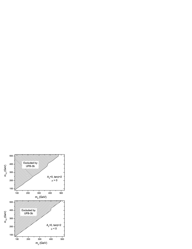
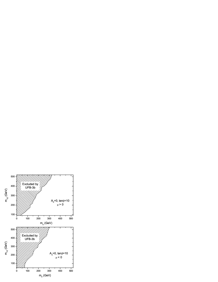
Figure 1: Exclusion plots in the $m_{0}$ vs $m_{1/2}$ plane for the UFB-3b direction

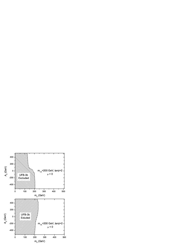
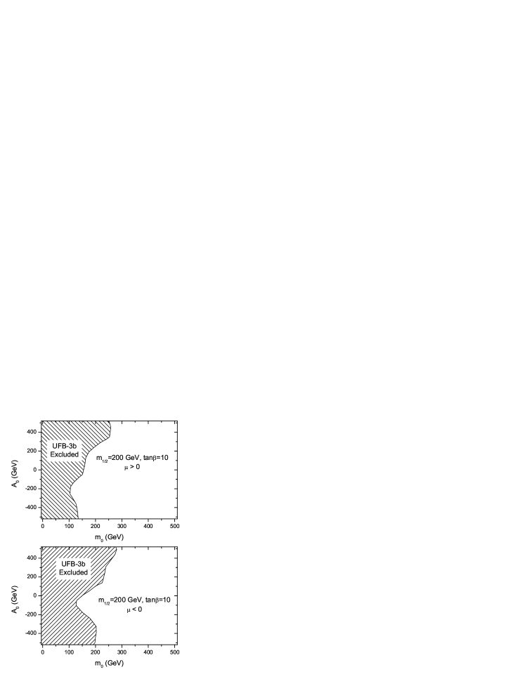
Figure 2: Exclusion plots in the $m_{0}$ vs $A_{0}$ plane for the UFB-3b direction

We fix $\tan\beta$ to be $2$ or $10$, and take $A_{0}=0$. Our search was performed in the range $(0,500)$ GeV for both axis and the grid was scanned with $25$ GeV resolution. In Fig. 1 the shaded regions to the left of the solid line display points where UFB-3b escapes were discovered. These parameter values with $m_{0}$ smaller than $m_{1/2}$ indicate that much of the mSUGRA parameter space associated with light sleptons is ruled out. It is also worth noting that higher values of $\tan\beta$ weaken these constraints.

Although Fig. 1 is plotted for $A_{0}=0$, a similar excluded region results for other choices of the $A_{0}$ parameter. An analogous plot in Fig. 2 displays the effect of variation in the trilinear $A_{0}$ parameter in combination with $m_{0}$ for fixed $m_{1/2}$ at $200$ GeV. Again, as usual, we fixed $\tan\beta$ to be $2$ or $10$. Performing a numerical minimization along the UFB-3b direction, unphysical configurations were found only for initial values taken from the shaded regions. Similarly, we find out that the vacuum constraints disfavor light slepton cases.

We have also examined a more general non-universal case coming from string models, which encompasses the special case where supersymmetry is broken in the dilaton sector. In the latter case one is led to GUT scale soft terms related by $m_{1/2}=-A_{0}=\sqrt{3}m_{0}$. However, in our examination we treat $m_{0}$ as a free parameter. We performed scans in the ($m_{0},m_{1/2}$) plane with the usual values for $\tan\beta$ ($2$ or $10$). Numerical minimization showed that for small $m_{0}$ much of the parameter space is excluded by the UFB-3b constraint, as shown in Fig. 3. Furthermore, it is easy to see that the so-called dilaton dominated scenario corresponds to a straight line located entirely inside the forbidden region.

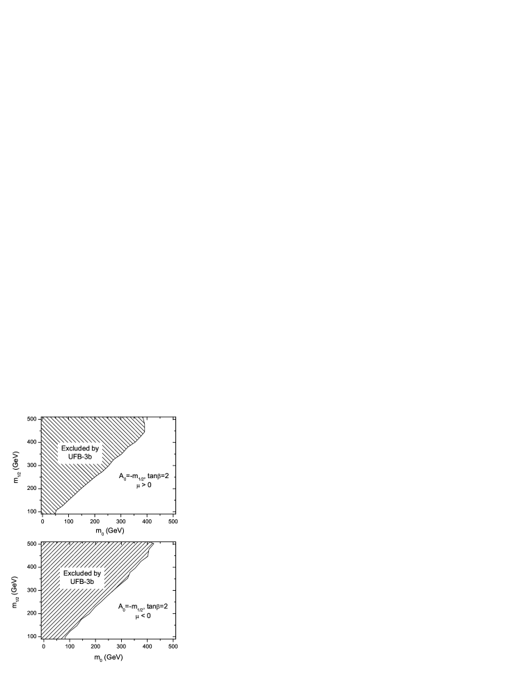
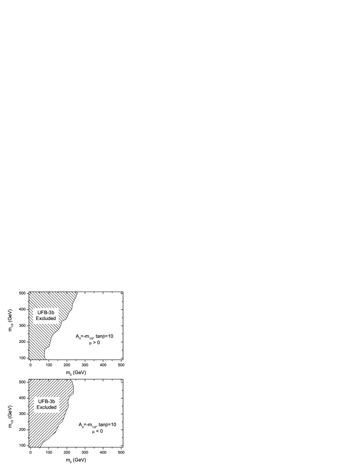
Figure 3: Exclusion plots in the $m_{0}$ vs $m_{1/2}$ plane with the additional constraint $A_{0}=-m_{1/2}$ for the UFB-3b direction

A similar scan in the parameter space of the MSSM has also been performed along the dangerous direction CCB-Eb. We considered again the three different regions depicted in Figs 1-3. Using the simplex minimization procedure and the one-loop expressions in Appendix E, we found no dangerous CCB minima. Tree level constraints described in Appendix B have also considered, as the numerical procedure scanned various field configurations and found that they are not violated for fields $|\phi|\sim A_{e}/Y_{e}\sim 10^{3}/10^{-5}$ GeV $\sim 10^{8}$ GeV. In great measure this is due to the large and positive contribution to the potential of the soft masses and especially $m_{1}^{2}$. Let us stress here that our renormalization scale choice depends on the field point we are. If at some field point $\phi_{0}$ the renormalization scale $Q^{*}_{0}=Q^{*}(\phi_{0})$ does reverse the inequality of a tree level constraint, then the tree level potential constructed from “soft” parameters at the specific scale $Q^{*}_{0}$ will be deeper than the physical vacuum for fields $|\phi_{d}|\sim A_{e}(Q^{*}_{0})/Y_{e}(Q^{*}_{0})$. In other words, tree level constraints signal an unphysical situation only if they are violated for fields of the order $\sim A_{e}(Q^{*})/Y_{e}(Q^{*})$.

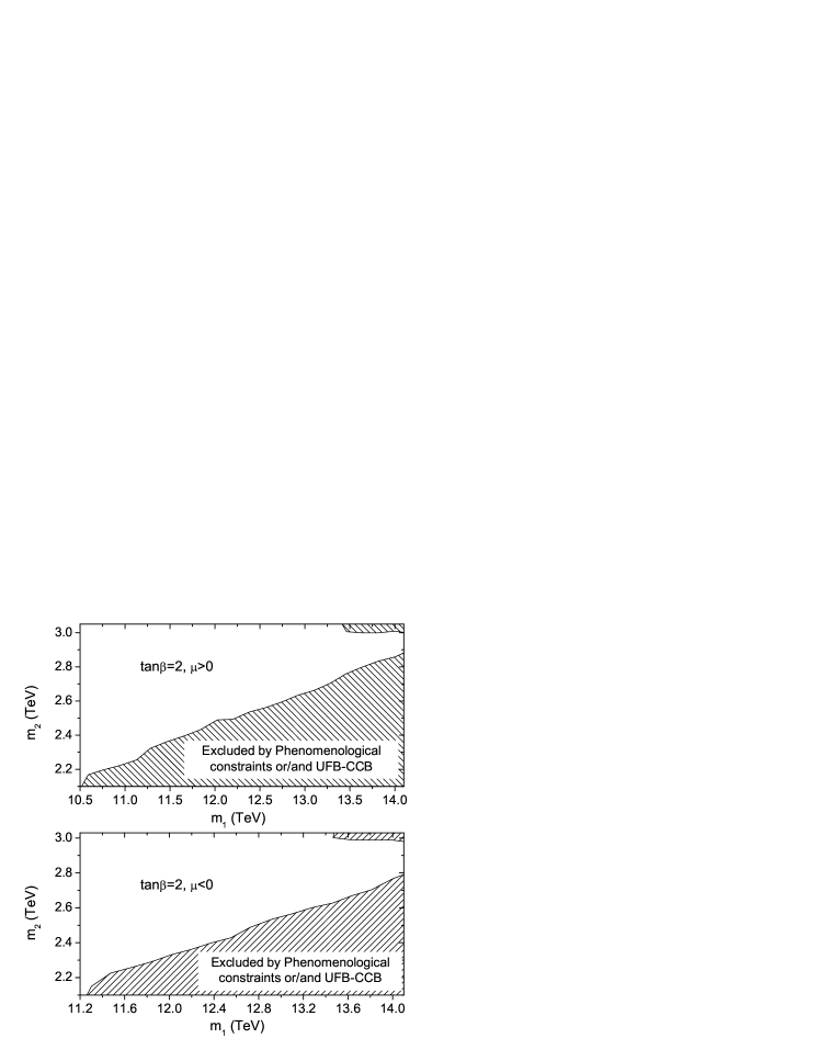
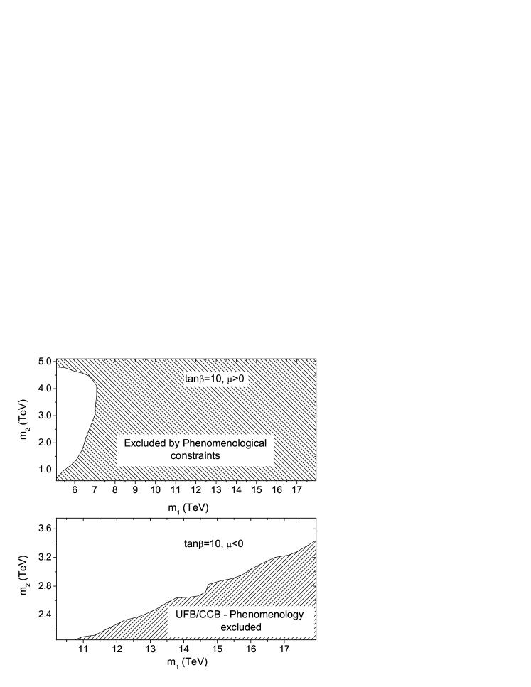
Figure 4: Exclusion plots for the $m_{1}$ vs $m_{2}$ plane in a brane world model.

We next focus our attention on the non-universal brane model and perform a scan for unphysical vacuua. In that case, due to non-universality, sparticles may generate too large flavor-changing (FC) effects but the specific brane model offers a mechanism for suppressing these dangerous processes. In this scenario, pushing the SUSY breaking scale at the first brane high enough ($m_{1}\simeq 10-20$ TeV), the masses of the first and second generations scalars will become sufficiently heavy to avoid the flavor problem. On the other hand, introducing a second SUSY breaking scale ($m_{2}$) attached to the second brane constrains the heavy scalars to be not much heavier than $1$ TeV or so to preserve the gauge hierarchy. We have performed scans in the $(m_{1},m_{2})$ plane for the values described above. Our results for $\tan\beta=2,10$ are shown in Fig. 4, where one can also see the regions excluded by phenomenological constraints or/and by unphysical vacuua driven radiatively by negative scalar mass eigenvalues. Note that in the case $\tan\beta=10,~{}\mu>0$ the parameter space is strongly restricted allowing only a very small “window” for phenomenology.

Unfortunately, an analytical treatment of these issues is tedious and leads to very unwieldy expressions [31]. Relaxing our preciseness requirements, we can intuitively realize the strength of a dangerous direction by resorting to the familiar tree level expressions. Constraints based on tree level logic have been thoroughly studied in the past [12, 13, 15] and our intention here is not to reproduce these analyses, but merely to use them as an alternative confirmation since our renormalized effective potential respects perturbation series hierarchy. Indeed, as one can see in Appendix A, the global minimum of Eq. (12) (UFB-1 case) is not deeper than the physical vacuum, a fact that has been also numerically justified at one-loop level.

One way to test reliability of the effective potential is by checking scale invariance [27, 31, 32]. In our case the chosen scale can not vary arbitrarily, since this endangers convergence of loop expansion. For very large values of scale $\theta$ steps in $V^{(1)}$ allow all heavy masses and loop corrections become huge. We have tried several scale prescriptions (various $\omega$ choices) and found that only the location of a UFB-3b escape is sensitive to scale variations. We believe that this sensitivity is due to cancellations that take place along a UFB-3b escape and higher loop effects. Since our expressions are only one-loop scale invariant, the higher loop difference is amplified by these cancellations and appears as a small “rotation” of the escape trajectory. The important point is that the physical picture remains unchanged: whatever $\omega(x)$ one chooses (within perturbativity constraints) cannot render an unstable potential stable and vice versa.

In the present work we mainly focus on an explicit treatment of the effect one loop radiative corrections may have on various UFB and CCB dangerous directions in supergravity models. Due to the intrinsic complexity of this subject, as well as the theoretical problem of multiple mass scales these issues have not been straightly touched upon in the past. Here for the first time, implementing a sophisticated threshold technique [17, 18] outlined in Sec. 5, we were able both to overcome the multiscale problem and deal explicitly with the radiative corrections. We believe that this is a more complete approach leading to more reliable results and corresponding plots. Practically, our improved results are in broad agreement with previous investigations [13, 15]. However, a more detailed comparison is highly non-trivial due to the variety of methods implemented by the various authors.

7 Conclusions

Minimal SUGRA scenarios provide a well motivated and phenomenologically viable framework of how weak scale supersymmetry might occur. Unfortunately, one has to pay the price of introducing extra degrees of freedom and new parameters leading to the appearance of new sources of flavor changing and CP violating processes, large number of new parameters and complicated scalar sector of the theory. On the other hand, the way low energy is related to the fundamental theory may shed some light to the solution of these problems.

In this paper, trying to constrain the parameter space of some mSUGRA models as described in introduction, we follow a strategy of finding regions in the general scalar field configuration space which have inferior values than the physical vacuum. The argument is that, if this configuration is not a minimum, an unbounded from below direction or a global minimum with charge and/or color broken surely exists somewhere and the associated point in parameter space should be excluded from consideration.

We have analyzed the relevant potentials employing the full one-loop radiative corrections in the calculation. Because of the various mass scales present in these models, renormalization group improvement of the potential has ambiguities and should be carefully treated. Implementing the decoupling theorem in a manner proposed by the authors of Ref. [17, 18], we treat the various particle thresholds as steps in the $\beta$-functions as well as in the one loop corrections of the scalar potential. We stress here the role played by the renormalization scale choice, as given in Sec. 5. It should be wisely chosen in order to eliminate heavy particles whose participation puts in danger the convergence of the loop expansion (i.e. $|V^{(1)}|\lesssim|V^{(0)}|$).

Employing the framework just stated and using numerical minimization procedure, we have performed an analysis of how the most dangerous directions put restrictions on the whole parameter space of the various models described. In both the MSSM case and the brane world scenario considered, these constraints turn out to be very strong, producing important bounds not only on the value of $A$ (soft trilinear coupling), but also on the values of $m_{1/2}$ (gaugino masses) and $m_{0}$ (scalar masses). Our analysis is summarized in Figs 1-4. As a general trend, the smaller the value of $m_{0}$ the more restrictive the constraints become.

Finally, we note that the more or less strict constraints derived here from non-standard vacuua are avoided if we adopt the idea [33] that we may indeed exist in a false vacuum and the tunneling rate from our present vacuum to a non-standard one might be small relative to the age of the universe. However, it is difficult to realize the circumstances under which the idea that we may live in a false, metastable vacuum could be reconciled with the existence of a small positive dark energy in the universe, either in the form of a constant vacuum energy/cosmological constant or in the form of a new scalar quintessence field, as the recent discoveries suggest [34].

Appendix A Analytic treatment of UFB-1 at tree level

In this appendix we compute the global minimum of the tree level effective potential along the UFB-1 direction. Assuming for simplicity real fields, the solution is based on the new “polar” variables $(R_{1},R_{2},\varphi,\theta)$ where

$$H_{1}=R_{1}\cos\varphi\qquad h_{1}=R_{1}\sin\varphi\qquad H_{2}=R_{2}\cos\theta\qquad h_{2}=R_{2}\sin\theta$$ (27)

Of course $R_{1}>0,R_{2}>0$ for an invertible transformation, thus the trivial case should be examined separately. If we take both or at least one $R$ trivial, we also find a trivial value for the potential extremum which is clearly above the physical vacuum shown in Eq. (10). Hence it is sufficient to minimize the function

$$V^{(0)}=m_{1}^{2}R_{1}^{2}+m_{2}^{2}R_{2}^{2}+2m_{3}^{2}R_{1}R_{2}\cos(\varphi+\theta)+\frac{{g_{2}^{2}}}{2}R_{1}^{2}R_{2}^{2}\sin^{2}(\varphi+\theta)+\frac{{g^{2}+g_{2}^{2}}}{8}(R_{1}^{2}-R_{2}^{2})^{2}$$ (28)

Solution of the minimization conditions leads to the following cases:

(I)

$R_{1}R_{2}\cos(\varphi+\theta)=2m_{3}^{2}/g_{2}^{2},~{}~{}~{}\partial_{R_{1}}V^{(0)}=0~{}\mbox{and}~{}\partial_{R_{2}}V^{(0)}=0~{}\mbox{with}~{}R_{1},R_{2}\neq 0$
Solving with respect to $R_{1},R_{2}$ we get $R_{1}^{2}=(m_{2}^{2}-m_{1}^{2})/g^{2}-(m_{1}^{2}+m_{2}^{2})/g_{2}^{2}$, and $R_{2}^{2}=(m_{1}^{2}-m_{2}^{2})/g^{2}-(m_{1}^{2}+m_{2}^{2})/g_{2}^{2}$. However, stability along $R_{1}=\pm R_{2},~{}\theta=\phi=0$ direction dictates positiveness of the $m_{1}^{2}+m_{2}^{2}$ combination $(m_{1}^{2}+m_{2}^{2}>2|m_{3}^{2}|)$ so one of $R_{1}^{2},R_{2}^{2}$ will be negative. Thus, no stationary solution exists or the potential is unbounded from below.

(II)

$\sin(\varphi+\theta)=0,~{}\partial_{R_{1}}V^{(0)}=0~{}\mbox{and}~{}\partial_{R_{2}}V^{(0)}=0~{}\mbox{with}~{}R_{1},R_{2}\neq 0$
In our conventions we always have $m_{3}^{2}<0$, so smaller values for $V^{(0)}$ are obtained for $\cos(\varphi+\theta)>0$. So we should take here $\cos(\varphi+\theta)=1$ (i.e. $\theta=-\varphi$). The rest of the extremum conditions will become

$$\begin{array}[]{c}m_{1}^{2}R_{1}+m_{3}^{2}R_{2}+\hat{g}^{2}R_{1}(R_{1}^{2}-R_{2}^{2})=0\\ m_{2}^{2}R_{2}+m_{3}^{2}R_{1}-\hat{g}^{2}R_{2}(R_{1}^{2}-R_{2}^{2})=0\\ \end{array}$$ (29)

where $\hat{g}^{2}=(g^{2}+g_{2}^{2})/4$. Solutions for the above system are well known [35]. If we define $t=R_{2}/R_{1}$ (obviously $t=1$ does not satisfy Eq. (29)), the solution in the ordinary case of radiative $SU(2)$ breaking $(m_{1}^{2}+m_{2}^{2}\pm 2m_{3}^{2}>0,~{}m_{1}^{2}>m_{2}^{2},~{}m_{1}^{2}m_{2}^{2}-m_{3}^{4}<0)$ is:

$$t = \frac{-m_{1}^{2}-m_{2}^{2}-\sqrt{(m_{1}^{2}+m_{2}^{2}+2m_{3}^{2})(m_{1}^{2}+m_{2}^{2}-2m_{3}^{2})}}{2m_{3}^{2}}$$

$$R_{1} = \sqrt{\frac{{m_{1}^{2}-m_{2}^{2}t^{2}}}{{\hat{g}^{2}(t^{4}-1)}}}$$ (30)

and the global minimum configuration is:

$$\left(\begin{array}[]{c}H_{1}\\ H_{2}\\ h_{1}\\ h_{2}\\ \end{array}\right)_{min}=\left(\begin{array}[]{c}R_{1}\cos\varphi\\ tR_{1}\cos\varphi\\ R_{1}\sin\varphi\\ -tR_{1}\sin\varphi\\ \end{array}\right)~{}~{}~{}~{}~{}~{}~{}~{}~{}~{}~{}\varphi\mbox{ arbitrary.}$$ (31)

It is trivial to show that the value at the minimum for this configuration coincides with the physical vacuum one of Eq. (10).

Appendix B Tree level constraints for CCB-Eb direction

Following closely the notation of [11, 12], we express all fields in Eq. (20) in terms of $|H_{1}|$, so that $|\tilde{\ell}_{1}|=\alpha|H_{1}|,~{}|\tilde{E}^{c}_{1}|=\beta|H_{1}|,~{}|H_{2}|=\gamma|H_{1}|$. Since the trilinear terms of our example have small coupling $(|Y_{e}|^{2}\ll 1)$, $D$-terms should be suppressed. This implies that $\alpha=\beta$ and $\alpha^{2}+\gamma^{2}=1$. To proceed further, two cases should be examined:

•

$\mathrm{sign}(A_{e})=-\mathrm{sign}(B)$ with $m_{3}^{2}=\mu B$, $\alpha=\sqrt{1-\gamma^{2}}$ and $0<|\gamma|<1$.
Then, all three trilinear terms can be made negative simultaneously and the tree level potential becomes

$$V_{\mathit{CCB-Eb}}^{(0)}=|Y_{e}|^{2}\alpha^{4}F(\alpha)|H_{1}|^{4}-2Y_{e}\hat{A}\alpha^{2}|H_{1}|^{3}+\hat{m}^{2}|H_{1}|^{2}$$ (32)

where $F(\alpha)=1+2/\alpha^{2}$, $\hat{A}=|A_{e}|+|\mu|\gamma$ and $\hat{m}^{2}=m_{1}^{2}+(m_{\tilde{L}_{1}}^{2}+m_{\tilde{E}^{c}_{1}}^{2})\alpha^{2}+m_{2}^{2}\gamma^{2}-2|m_{3}^{2}|\gamma$. Differentiating with respect to $|H_{1}|$ for fixed values of $\gamma$, we find besides the trivial extremum the following local minimum for Eq. (32)

$$|H_{1}|_{\mathit{ext}}=\frac{3\hat{A}}{4Y_{e}\alpha^{2}F(\alpha)}\left[1+\sqrt{1-\frac{8\hat{m}^{2}F(\alpha)}{9\hat{A}^{2}}}\right]$$ (33)

Note that the typical vevs are of order $|A_{e}|/Y_{e}$. The corresponding value of the potential is

$$V_{\mathit{ext}}=-\frac{1}{2}\alpha^{2}|H_{1}|_{\mathit{ext}}^{2}\left[Y_{e}\hat{A}|H_{1}|_{\mathit{ext}}-\frac{\hat{m}^{2}}{\alpha^{2}}\right]$$ (34)

and the constraint to avoid a deeper configuration than the physical vacuum Eq. (10) of the theory reads $\hat{A}^{2}\leq F\hat{m}^{2}$ i.e.

$$(|A_{e}|+|\mu|\gamma)^{2}\leq\left(1+\frac{2}{\alpha^{2}}\right)\left(m_{1}^{2}+(m_{\tilde{L}_{1}}^{2}+m_{\tilde{E}^{c}_{1}}^{2})\alpha^{2}+m_{2}^{2}\gamma^{2}-2|m_{3}^{2}|\gamma\right)$$ (35)

•

$\mathrm{sign}(A_{e})=\mathrm{sign}(B)$ with $\alpha=\sqrt{1-\gamma^{2}}$ and $0<|\gamma|<1$.
Similarly the relevant constraints are

$$(|A_{e}|-|\mu|\gamma)^{2} \leq \left(1+\frac{2}{\alpha^{2}}\right)\left(m_{1}^{2}+(m_{\tilde{L}_{1}}^{2}+m_{\tilde{E}^{c}_{1}}^{2})\alpha^{2}+m_{2}^{2}\gamma^{2}-2|m_{3}^{2}|\gamma\right)$$ (36)

$$(|A_{e}|+|\mu|\gamma)^{2} \leq \left(1+\frac{2}{\alpha^{2}}\right)\left(m_{1}^{2}+(m_{\tilde{L}_{1}}^{2}+m_{\tilde{E}^{c}_{1}}^{2})\alpha^{2}+m_{2}^{2}\gamma^{2}+2|m_{3}^{2}|\gamma\right)$$ (37)

Appendix C Field dependent mass matrix elements for UFB-1

We cite here all the necessary mass matrix elements used in the definition of the one loop effective potential. Let $\psi^{r},~{}r=1,2,3$ stands for a Yukawa ($Y$) or a trilinear soft coupling ($A$). The following notation is used throughout $\psi_{u}^{r}\equiv(\psi_{u},~{}\psi_{c},~{}\psi_{t})$ and $\psi_{d}^{r}\equiv(\psi_{d},~{}\psi_{s},~{}\psi_{b})$.
• Gauge Bosons ($\Omega=C=1$)

$$\mathcal{L}_{V}=\frac{1}{2}\left(W_{\mu}^{+}~{}W_{\mu}^{-}~{}A_{\mu}~{}Z_{\mu}\right)[\mathcal{M}_{V}^{2}]\left(\begin{array}[]{c}W_{\mu}^{-}\\ W_{\mu}^{+}\\ A_{\mu}\\ Z_{\mu}\end{array}\right),~{}~{}~{}~{}~{}~{}~{}~{}[\mathcal{M}_{V}^{2}]=\left(\begin{array}[]{cccc}V_{1}&0&V_{2}&V_{3}\\ 0&V_{1}&V_{2}^{*}&V_{3}^{*}\\ V_{2}^{*}&V_{2}&V_{4}&V_{5}\\ V_{3}^{*}&V_{3}&V_{5}&V_{6}\end{array}\right)$$

$$V_{1} = \frac{g^{2}_{2}}{2}\left(|H_{1}|^{2}+|H_{2}|^{2}+|h_{1}|^{2}+|h_{2}|^{2}\right)\qquad V_{2}=-\frac{eg_{2}}{\sqrt{2}}\left(H^{*}_{1}h_{1}-H_{2}h^{*}_{2}\right)$$

$$V_{3} = \frac{eg}{\sqrt{2}}\left(H^{*}_{1}h_{1}-H_{2}h^{*}_{2}\right)\qquad\qquad\quad\,V_{4}=2e^{2}\left(|h_{1}|^{2}+|h_{2}|^{2}\right)$$

$$V_{5} = -gg_{2}\frac{g^{2}-g_{2}^{2}}{g^{2}+g_{2}^{2}}\left(|h_{1}|^{2}+|h_{2}|^{2}\right)$$

$$V_{6} = \frac{g^{2}+g_{2}^{2}}{2}\left[|H_{1}|^{2}+|H_{2}|^{2}+\left(\frac{g^{2}-g_{2}^{2}}{g^{2}+g_{2}^{2}}\right)^{2}\left(|h_{1}|^{2}+|h_{2}|^{2}\right)\right]$$

where $e=gg_{2}/\sqrt{g^{2}+g_{2}^{2}}.$
• Leptons $(\Omega=C=1)$

$$M_{e}^{2}=|Y_{e}|^{2}(|H_{1}|^{2}+|h_{1}|^{2})~{}\qquad~{}M_{\mu}^{2}=|Y_{\mu}|^{2}(|H_{1}|^{2}+|h_{1}|^{2})~{}\qquad~{}M_{\tau}^{2}=|Y_{\tau}|^{2}(|H_{1}|^{2}+|h_{1}|^{2})$$

• Quarks ($\Omega=2,~{}C=3$)

$$\mathcal{L}_{L}=-\sum_{r,a=1}^{3}\left(u_{ra}^{c}~{}d_{ra}^{c}\right)[\mathcal{M}_{Q}]_{r}\left(\begin{array}[]{c}u_{r}^{a}\\ d_{r}^{a}\end{array}\right)~{}~{}\mbox{where}~{}~{}[\mathcal{M}_{Q}]_{r}=\left(\begin{array}[]{cc}-Y_{u}^{r}H_{2}&Y_{u}^{r}h_{2}\\ -Y_{d}^{r}h_{1}&Y_{d}^{r}H_{1}\end{array}\right)$$

The necessary eigenvalues should be computed from $\mathcal{M}_{Q}\mathcal{M}_{Q}^{{\dagger}}$.
• Higgsinos ($\Omega=C=1$)

$$\mathcal{L}_{\tilde{H}}=-\frac{1}{2}\chi^{T}[\mathcal{M}_{\tilde{H}}]\chi~{}~{}\mbox{where}~{}~{}~{}\chi^{T}=\left(\tilde{H}^{0}_{1}~{}\tilde{H}_{1}^{-}~{}\tilde{H}_{2}^{+}~{}\tilde{H}^{0}_{2}~{}\tilde{B}~{}\tilde{W}^{+}~{}\tilde{W}^{-}~{}\tilde{W}^{(3)}\right)\mbox{ and}$$

$~{}[\mathcal{M}_{\tilde{H}}]=\left(\begin{array}[]{cc}S_{1}&S_{2}^{*}\\ S_{2}^{\dagger}&S_{4}\end{array}\right)\mbox{with}~{}~{}~{}~{}S_{1}=\left(\begin{array}[]{rccr}0&0&0&-\mu\\ 0&0&\mu&0\\ 0&\mu&0&0\\ -\mu&0&0&0\end{array}\right),$

$$S_{2}=\left(\begin{array}[]{cccc}\frac{g}{\sqrt{2}}H_{1}&0&-g_{2}h_{1}&-\frac{g_{2}}{\sqrt{2}}H_{1}\\ \frac{g}{\sqrt{2}}h_{1}&-g_{2}H_{1}&0&\frac{g_{2}}{\sqrt{2}}h_{1}\\ -\frac{g}{\sqrt{2}}h_{2}&0&-g_{2}H_{2}&-\frac{g_{2}}{\sqrt{2}}h_{2}\\ -\frac{g}{\sqrt{2}}H_{2}&-g_{2}h_{2}&0&\frac{g_{2}}{\sqrt{2}}H_{2}\end{array}\right),~{}~{}~{}S_{4}=\left(\begin{array}[]{cccc}M_{1}&0&0&0\\ 0&0&M_{2}&0\\ 0&M_{2}&0&0\\ 0&0&0&M_{2}\end{array}\right).$$

• Sleptons $(\tilde{L}^{T}\equiv(~{}\tilde{\nu}~{}~{}\tilde{\ell}~{})~{}\Omega=2,~{}C=1)$

$$\mathcal{L}_{\tilde{L}}=-\sum_{r=1}^{3}\left(\tilde{\nu}_{r}~{}\tilde{\ell}_{r}~{}\tilde{E}^{c*}_{r}\right)[\mathcal{M}_{\tilde{L}}^{2}]_{r}\left(\begin{array}[]{c}\tilde{\nu}_{r}^{*}\\ \tilde{\ell}_{r}^{*}\\ \tilde{E}^{c}_{r}\end{array}\right)~{}~{}\mbox{where}~{}~{}[\mathcal{M}_{\tilde{L}}^{2}]_{r}=\left(\begin{array}[]{ccc}B_{1}^{r}&B_{2}^{r}&A_{1}^{r}\\ B_{2}^{r*}&B_{3}^{r}&A_{2}^{r}\\ A_{1}^{r*}&A_{2}^{r*}&A_{3}^{r}\end{array}\right).$$

We give below the relevant entries

$$A_{1}^{r} = Y_{e}^{r}(\mu h^{*}_{2}-A_{e}^{r}h_{1})\qquad\qquad\qquad A_{2}^{r}=Y_{e}^{r}(\mu H^{*}_{2}+A_{e}^{r}H_{1})$$

$$A_{3}^{r} = m_{\tilde{E}^{c}_{r}}^{2}+|Y_{e}^{r}|^{2}\left(|H_{1}|^{2}+|h_{1}|^{2}\right)-\frac{g^{2}}{2}\left(|H_{1}|^{2}+|h_{1}|^{2}-|H_{2}|^{2}-|h_{2}|^{2}\right)$$

$$B_{1}^{r} = m_{\tilde{L}_{r}}^{2}+|Y_{e}^{r}h_{1}|^{2}+\frac{g^{2}+g_{2}^{2}}{4}\left(|H_{1}|^{2}-|H_{2}|^{2}\right)+\frac{g^{2}-g_{2}^{2}}{4}\left(|h_{1}|^{2}-|h_{2}|^{2}\right)$$

$$B_{2}^{r} = \left(\frac{g_{2}^{2}}{2}-|Y_{e}^{r}|^{2}\right)H^{*}_{1}h_{1}+\frac{g_{2}^{2}}{2}H_{2}h^{*}_{2}$$

$$B_{3}^{r} = m_{\tilde{L}_{r}}^{2}+|Y_{e}^{r}H_{1}|^{2}+\frac{g^{2}-g_{2}^{2}}{4}\left(|H_{1}|^{2}-|H_{2}|^{2}\right)+\frac{g^{2}+g_{2}^{2}}{4}\left(|h_{1}|^{2}-|h_{2}|^{2}\right)$$

• Squarks $(\tilde{Q}^{T}\equiv(~{}\tilde{u}~{}~{}\tilde{d}~{})~{}\Omega=2,~{}C=3)$

$$\mathcal{L}_{\tilde{Q}}=-\sum_{a,r=1}^{3}\left(\tilde{u}_{r}^{a}~{}\tilde{d}_{r}^{a}~{}\tilde{U}^{c*}_{ra}~{}\tilde{D}^{c*}_{ra}\right)[M_{\tilde{Q}}^{2}]_{r}\left(\begin{array}[]{c}\tilde{u}_{r}^{a*}\\ \tilde{d}_{r}^{a*}\\ \tilde{U}^{c}_{ra}\\ \tilde{D}^{c}_{ra}\end{array}\right)~{}~{}\mbox{where}~{}~{}[M_{\tilde{Q}}^{2}]_{r}=\left(\begin{array}[]{cccc}\Lambda_{1}^{r}&\Lambda_{2}^{r}&K_{5}^{r}&K_{7}^{r}\\ \Lambda_{2}^{r*}&\Lambda_{3}^{r}&K_{6}^{r}&K_{8}^{r}\\ K_{5}^{r*}&K_{6}^{r*}&K_{1}^{r}&K_{2}^{r}\\ K_{7}^{r*}&K_{8}^{r*}&K_{2}^{r*}&K_{3}^{r}\end{array}\right)$$

where

$$\Lambda_{1}^{r} = m_{\tilde{Q}_{r}}^{2}+|Y_{u}^{r}H_{2}|^{2}+|Y_{d}^{r}h_{1}|^{2}-G^{-}\left(|H_{1}|^{2}-|H_{2}|^{2}\right)-G^{+}\left(|h_{1}|^{2}-|h_{2}|^{2}\right)$$

$$\Lambda_{2}^{r} = \left(\frac{g_{2}^{2}}{2}-|Y_{d}^{r}|^{2}\right)H^{*}_{1}h_{1}+\left(\frac{g_{2}^{2}}{2}-|Y_{u}^{r}|^{2}\right)H_{2}h^{*}_{2}$$

$$\Lambda_{3}^{r} = m_{\tilde{Q}_{r}}^{2}+|Y_{d}^{r}H_{1}|^{2}+|Y_{u}^{r}h_{2}|^{2}-G^{+}\left(|H_{1}|^{2}-|H_{2}|^{2}\right)-G^{-}\left(|h_{1}|^{2}-|h_{2}|^{2}\right)$$

$$K_{1}^{r} = m_{\tilde{U}^{c}_{r}}^{2}+|Y_{u}^{r}|^{2}\left(|H_{2}|^{2}+|h_{2}|^{2}\right)+\frac{g^{2}}{3}\left(|H_{1}|^{2}+|h_{1}|^{2}-|H_{2}|^{2}-|h_{2}|^{2}\right)$$

$$K_{2}^{r} = Y_{u}^{r}Y_{d}^{r}\left(H_{1}h^{*}_{2}+H^{*}_{2}h_{1}\right)$$

$$K_{3}^{r} = m_{\tilde{D}^{c}_{r}}^{2}+|Y_{d}^{r}|^{2}\left(|H_{1}|^{2}+|h_{1}|^{2}\right)-\frac{g^{2}}{6}\left(|H_{1}|^{2}+|h_{1}|^{2}-|H_{2}|^{2}-|h_{2}|^{2}\right)$$

and by definition $G^{+}=(g^{2}+3g_{2}^{2})/12~{}~{}~{}~{}~{}G^{-}=(g^{2}-3g_{2}^{2})/12.$ Besides

$$\begin{array}[]{cccrc}K_{5}^{r}&=&-Y_{u}^{r}(\mu H^{*}_{1}+A_{u}^{r}H_{2})&K_{6}^{r}=&-Y_{u}^{r}(\mu h^{*}_{1}-A_{u}^{r}h_{2})\\ K_{7}^{r}&=&Y_{d}^{r}(\mu h^{*}_{2}-A_{d}^{r}h_{1})&K_{8}^{r}=&Y_{d}^{r}(\mu H^{*}_{2}+A_{d}^{r}H_{1})\end{array}$$

• Higgs $(\Omega=1,~{}C=1)$

$$\mathcal{L}_{H}=-\frac{1}{2}\phi^{T}[\mathcal{M}_{H}^{2}]\phi^{*}~{}~{}\mbox{where}~{}~{}[\mathcal{M}_{H}^{2}]=\left(\begin{array}[]{cc}T_{1}&T_{2}^{\dagger}\\ T_{2}&T_{1}^{*}\end{array}\right)$$

with

$$T_{1}=\left(\begin{array}[]{cccc}R_{1}&R_{2}&R_{4}&R_{5}\\ R_{2}^{*}&R_{3}&R_{6}&R_{7}\\ R_{4}^{*}&R_{6}^{*}&R_{8}&R_{9}\\ R_{5}^{*}&R_{7}^{*}&R_{9}^{*}&R_{10}\end{array}\right),\qquad\qquad T_{2}=\left(\begin{array}[]{cccc}Q_{1}&Q_{2}&Q_{4}&Q_{5}\\ Q_{2}&Q_{3}&Q_{6}&Q_{7}\\ Q_{4}&Q_{6}&Q_{8}&Q_{9}\\ Q_{5}&Q_{7}&Q_{9}&Q_{10}\end{array}\right)$$

and $\phi^{T}=\left(\varphi^{T}~{}\varphi^{T*}\right),~{}~{}\varphi^{T}=\left(H_{1}^{0}~{}H_{1}^{-}~{}H_{2}^{+}~{}H_{2}^{0}\right).$ Additionally

$$R_{1} = m_{1}^{2}+\frac{g^{2}+g_{2}^{2}}{4}\left(2|H_{1}|^{2}+|h_{1}|^{2}-|H_{2}|^{2}-|h_{2}|^{2}\right)+\frac{g_{2}^{2}}{2}|h_{2}|^{2}$$

$$R_{2} = \frac{g^{2}+g_{2}^{2}}{4}H^{*}_{1}h_{1}+\frac{g_{2}^{2}}{2}H_{2}h^{*}_{2}$$

$$R_{3} = m_{1}^{2}+\frac{g^{2}+g_{2}^{2}}{4}\left(|H_{1}|^{2}+2|h_{1}|^{2}-|H_{2}|^{2}-|h_{2}|^{2}\right)+\frac{g_{2}^{2}}{2}|H_{2}|^{2}$$

$$R_{4} = \frac{g_{2}^{2}}{2}H_{2}h^{*}_{1}-\frac{g^{2}-g_{2}^{2}}{4}H^{*}_{1}h_{2}\qquad\qquad R_{5}=-\frac{g^{2}+g_{2}^{2}}{4}H^{*}_{1}H_{2}$$

$$R_{6} = -\frac{g^{2}+g_{2}^{2}}{4}h^{*}_{1}h_{2}\qquad\qquad~{}~{}~{}~{}~{}~{}~{}~{}~{}~{}~{}~{}\,R_{7}=-\frac{g^{2}-g_{2}^{2}}{4}H_{2}h^{*}_{1}+\frac{g_{2}^{2}}{2}H^{*}_{1}h_{2}$$

$$R_{8} = m_{2}^{2}+\frac{g^{2}+g_{2}^{2}}{4}\left(|H_{2}|^{2}+2|h_{2}|^{2}-|H_{1}|^{2}-|h_{1}|^{2}\right)+\frac{g_{2}^{2}}{2}|H_{1}|^{2}$$

$$R_{9} = \frac{g_{2}^{2}}{2}H^{*}_{1}h_{1}+\frac{g^{2}+g_{2}^{2}}{4}H_{2}h^{*}_{2}$$

$$R_{10} = m_{2}^{2}+\frac{g^{2}+g_{2}^{2}}{4}\left(2|H_{2}|^{2}+|h_{2}|^{2}-|H_{1}|^{2}-|h_{1}|^{2}\right)+\frac{g_{2}^{2}}{2}|h_{1}|^{2}$$

and the matrix element for $T_{2}$ are

$$\begin{array}[]{llll}~{}~{}~{}~{}Q_{1}=&\displaystyle\frac{g^{2}+g_{2}^{2}}{4}(H_{1})^{2}&Q_{2}=&\displaystyle\frac{g^{2}+g_{2}^{2}}{4}H_{1}h_{1}\\[8.53581pt] ~{}~{}~{}~{}Q_{3}=&\displaystyle\frac{g^{2}+g_{2}^{2}}{4}(h_{1})^{2}&Q_{4}=&-\displaystyle\frac{g^{2}-g_{2}^{2}}{4}H_{1}h_{2}\\[8.53581pt] ~{}~{}~{}~{}Q_{5}=&\displaystyle m_{3}^{2}-\frac{g^{2}+g_{2}^{2}}{4}H_{1}H_{2}+\frac{g_{2}^{2}}{2}h_{1}h_{2}&Q_{6}=&\displaystyle-m_{3}^{2}-\frac{g^{2}+g_{2}^{2}}{4}h_{1}h_{2}+\frac{g_{2}^{2}}{2}H_{1}H_{2}\\[8.53581pt] ~{}~{}~{}~{}Q_{7}=&\displaystyle-\frac{g^{2}-g_{2}^{2}}{4}H_{2}h_{1}&Q_{8}=&\displaystyle\frac{g^{2}+g_{2}^{2}}{4}(h_{2})^{2}\\[8.53581pt] ~{}~{}~{}~{}Q_{9}=&\displaystyle\frac{g^{2}+g_{2}^{2}}{4}H_{2}h_{2}&Q_{10}=&\displaystyle\frac{g^{2}+g_{2}^{2}}{4}(H_{2})^{2}\\[8.53581pt] \end{array}$$

Appendix D Field dependent mass matrix elements for UFB-3b

Here we present the mass matrix elements needed in the one loop effective potential expression. We use the same notation as in Appendix C.
• Gauge Bosons $(\Omega_{W^{\pm}}=2,~{}\Omega_{A,Z}=1,~{}C=1)$

$$\mathcal{L}_{V}=M_{W^{\pm}}^{2}W_{\mu}^{+}W^{-\mu}+\frac{1}{2}\left(A_{\mu}~{}Z_{\mu}\right)[M^{2}_{(A,Z)}]\left(\begin{array}[]{c}A^{\mu}\\ Z^{\mu}\end{array}\right),\qquad[M^{2}_{(A,Z)}]=\left(\begin{array}[]{cc}V_{2}&V_{3}\\ V_{3}&V_{4}\end{array}\right)$$

$$M_{W^{\pm}}^{2} = \frac{g_{2}^{2}}{2}\left(|H_{2}|^{2}+|\tilde{\nu}_{2}|^{2}+|\tilde{\ell}_{3}|^{2}\right)$$

$$V_{2} = 2e^{2}\left(|\tilde{\ell}_{3}|^{2}+|\tilde{E}^{c}_{3}|^{2}\right)~{}~{}~{}~{}~{}~{}~{}~{}~{}~{}V_{3}=gg_{2}\left[|\tilde{\ell}_{3}|^{2}-2\sin^{2}\theta_{W}\left(|\tilde{E}^{c}_{3}|^{2}+|\tilde{\ell}_{3}|^{2}\right)\right]$$

$$V_{4} = \frac{g^{2}+g_{2}^{2}}{2}\left[|H_{2}|^{2}+|\tilde{\nu}_{2}|^{2}+(1-2\sin^{2}\theta_{W})^{2}|\tilde{\ell}_{3}|^{2}+4\sin^{4}\theta_{W}|\tilde{E}^{c}_{3}|^{2}\right]$$

where $e=gg_{2}/\sqrt{g^{2}+g_{2}^{2}}$ and $\sin\theta_{W}=e/g_{2}.$
• Quarks $(\Omega=2,~{}C=3)$

$$M_{u}^{2}=|Y_{u}H_{2}|^{2}~{}\qquad~{}M_{c}^{2}=|Y_{c}H_{2}|^{2}~{}\qquad~{}M_{t}^{2}=|Y_{t}H_{2}|^{2}$$

• Leptons - Higgsinos $(\Omega=1,~{}C=1)$

$$\mathcal{L}_{(L,\tilde{H})}=-\frac{1}{2}\psi_{1}^{T}[M_{1}^{f}]\psi_{1}-\frac{1}{2}\psi_{2}^{T}[M_{2}^{f}]\psi_{2}$$

where $\psi_{1}^{T}=\left(\nu_{\mu}~{}\tau~{}\tau^{c}~{}\tilde{H}_{2}^{0}~{}\tilde{H}_{1}^{0}~{}\tilde{B}~{}\tilde{W}^{(3)}\right)$ and $\psi_{2}^{T}=\left(\nu_{\tau}~{}\mu~{}\mu^{c}~{}\tilde{H}_{2}^{+}~{}\tilde{H}_{1}^{-}~{}\tilde{W}^{+}~{}\tilde{W}^{-}\right).$ Besides

$$[M_{1}^{f}]=\left(\begin{array}[]{ccccccc}0&0&0&0&0&\frac{g}{\sqrt{2}}\tilde{\nu}^{*}_{2}&-\frac{g_{2}}{\sqrt{2}}\tilde{\nu}^{*}_{2}\\ 0&0&0&0&Y_{\tau}\tilde{E}^{c}_{3}&\frac{g}{\sqrt{2}}\tilde{\ell}^{*}_{3}&\frac{g_{2}}{\sqrt{2}}\tilde{\ell}^{*}_{3}\\ 0&0&0&0&Y_{\tau}\tilde{\ell}_{3}&-\sqrt{2}g\tilde{E}^{c*}_{3}&0\\ 0&0&0&0&\mu&-\frac{g}{\sqrt{2}}H^{*}_{2}&\frac{g_{2}}{\sqrt{2}}H^{*}_{2}\\ 0&Y_{\tau}\tilde{E}^{c}_{3}&Y_{\tau}\tilde{\ell}_{3}&\mu&0&0&0\\ \frac{g}{\sqrt{2}}\tilde{\nu}^{*}_{2}&\frac{g}{\sqrt{2}}\tilde{\ell}^{*}_{3}&-\sqrt{2}g\tilde{E}^{c*}_{3}&-\frac{g}{\sqrt{2}}H^{*}_{2}&0&-M_{1}&0\\ -\frac{g_{2}}{\sqrt{2}}\tilde{\nu}^{*}_{2}&\frac{g_{2}}{\sqrt{2}}\tilde{\ell}^{*}_{3}&0&\frac{g_{2}}{\sqrt{2}}H^{*}_{2}&0&0&-M_{2}\end{array}\right)$$

$$[M_{2}^{f}]=\left(\begin{array}[]{ccccccc}0&0&0&0&-Y_{\tau}\tilde{E}^{c}_{3}&0&-g_{2}\tilde{\ell}^{*}_{3}\\ 0&0&0&0&0&-g_{2}\tilde{\nu}^{*}_{2}&0\\ 0&0&0&0&-Y_{\mu}\tilde{\nu}_{2}&0&0\\ 0&0&0&0&-\mu&0&-g_{2}H^{*}_{2}\\ -Y_{\tau}\tilde{E}^{c}_{3}&0&-Y_{\mu}\tilde{\nu}_{2}&-\mu&0&0&0\\ 0&-g_{2}\tilde{\nu}^{*}_{2}&0&0&0&0&-M_{2}\\ -g_{2}\tilde{\ell}^{*}_{3}&0&0&-g_{2}H^{*}_{2}&0&-M_{2}&0\end{array}\right)$$

• Squarks $(\tilde{Q}^{T}\equiv(~{}\tilde{u}~{}~{}\tilde{d}~{}),~{}\Omega=2,~{}C=3)$

$$\mathcal{L}_{\tilde{Q}}=-\sum_{r,a=1}^{3}\left(\tilde{U}^{c}_{ra}~{}\tilde{u}_{r}^{a*}\right)[M_{1}^{2}]\left(\begin{array}[]{c}\tilde{U}^{c*}_{ra}\\ \tilde{u}_{r}^{a}\end{array}\right)-\sum_{r,a=1}^{3}\left(\tilde{D}^{c}_{ra}~{}\tilde{d}_{r}^{a*}\right)[M_{2}^{2}]\left(\begin{array}[]{c}\tilde{D}^{c*}_{ra}\\ \tilde{d}_{r}^{a}\end{array}\right)$$

where $[M_{1}^{2}]=\left(\begin{array}[]{cc}K_{1}^{r}&K_{4}^{r}\\ K_{4}^{r*}&\Lambda_{1}^{r}\end{array}\right)$ and $[M_{2}^{2}]=\left(\begin{array}[]{cc}K_{2}^{r}&K_{5}^{r}\\ K_{5}^{r*}&\Lambda_{2}^{r}\end{array}\right).$ The relevant quantities are

$$K_{1}^{r} = m_{\tilde{U}^{c}_{r}}^{2}+|Y_{u}^{r}H_{2}|^{2}-\frac{g^{2}}{3}\left(2|\tilde{E}^{c}_{3}|^{2}+|H_{2}|^{2}-|\tilde{\nu}_{2}|^{2}-|\tilde{\ell}_{3}|^{2}\right)$$

$$K_{4}^{r} = -Y_{u}^{r}A_{u}^{r}H_{2}$$

$$\Lambda_{1}^{r} = m_{\tilde{Q}_{r}}^{2}+|Y_{u}^{r}H_{2}|^{2}+\frac{g^{2}}{6}\left(|\tilde{E}^{c}_{3}|^{2}-|\tilde{\ell}_{3}|^{2}\right)+\frac{g^{2}-3g_{2}^{2}}{12}\left(|H_{2}|^{2}+|\tilde{\ell}_{3}|^{2}-|\tilde{\nu}_{2}|^{2}\right)$$

$$K_{2}^{r} = m_{\tilde{D}^{c}_{r}}^{2}+\frac{g^{2}}{6}\left(2|\tilde{E}^{c}_{3}|^{2}+|H_{2}|^{2}-|\tilde{\nu}_{2}|^{2}-|\tilde{\ell}_{3}|^{2}\right)$$

$$K_{5}^{r} = Y_{d}^{r}(\mu H^{*}_{2}+Y_{\tau}\tilde{\ell}^{*}_{3}\tilde{E}^{c*}_{3})$$

$$\Lambda_{2}^{r} = m_{\tilde{Q}_{r}}^{2}+\frac{g^{2}}{6}\left(|\tilde{E}^{c}_{3}|^{2}-|\tilde{\ell}_{3}|^{2}\right)+\frac{g^{2}+3g_{2}^{2}}{12}\left(|H_{2}|^{2}+|\tilde{\ell}_{3}|^{2}-|\tilde{\nu}_{2}|^{2}\right)$$

• Sleptons - Higgses $(\tilde{L}^{T}\equiv(~{}\tilde{\nu}~{}~{}\tilde{\ell}~{}))$

$$\mathcal{L}_{(\tilde{L},H)}=-M^{2}|\tilde{\nu}_{1}|^{2}-\left(\tilde{E}^{c}_{1}~{}\tilde{\ell}_{1}^{*}\right)[M_{s_{1}}^{2}]\left(\begin{array}[]{c}\tilde{E}^{c*}_{1}\\ \tilde{\ell}_{1}\end{array}\right)-\chi^{T}[M_{s_{2}}^{2}]\chi^{*}-\frac{1}{2}\phi^{T}[M_{s_{3}}^{2}]\phi^{*}$$

where $\chi^{T}=\left(H_{2}^{+}~{}\tilde{E}^{c}_{2}~{}\tilde{\nu}_{3}~{}H_{1}^{-*}~{}\tilde{\ell}_{2}^{*}\right)$ and $\phi^{T}=\left(\xi^{T}~{}\xi^{T*}\right),~{}\xi^{T}=\left(H_{1}^{0}~{}H_{2}^{0}~{}\tilde{E}^{c}_{3}~{}\tilde{\nu}_{2}~{}\tilde{\ell}_{3}\right).$

$$M^{2}=m_{\tilde{L}_{1}}^{2}+\frac{g^{2}}{2}\left(|\tilde{\ell}_{3}|^{2}-|\tilde{E}^{c}_{3}|^{2}\right)+\frac{g^{2}+g_{2}^{2}}{4}\left(|\tilde{\nu}_{2}|^{2}-|\tilde{\ell}_{3}|^{2}-|H_{2}|^{2}\right)~{}~{}~{}~{}~{}~{}(\Omega=2,~{}C=1).$$

On the other hand $[M_{s_{1}}^{2}]=\left(\begin{array}[]{cc}A_{1}&A_{2}\\ A_{2}^{*}&A_{3}\end{array}\right)~{}(\Omega=2,~{}C=1)$ with

$$A_{1} = m_{\tilde{E}^{c}_{1}}^{2}+\frac{g^{2}}{2}\left(2|\tilde{E}^{c}_{3}|^{2}+|H_{2}|^{2}-|\tilde{\nu}_{2}|^{2}-|\tilde{\ell}_{3}|^{2}\right)~{}~{}~{}~{}~{}~{}~{}~{}A_{2}=Y_{e}(\mu H^{*}_{2}+Y_{\tau}\tilde{\ell}^{*}_{3}\tilde{E}^{c*}_{3})$$

$$A_{3} = m_{\tilde{L}_{1}}^{2}+\frac{g^{2}}{2}\left(|\tilde{\ell}_{3}|^{2}-|\tilde{E}^{c}_{3}|^{2}\right)+\frac{g^{2}-g_{2}^{2}}{4}\left(|\tilde{\nu}_{2}|^{2}-|\tilde{\ell}_{3}|^{2}-|H_{2}|^{2}\right).$$

Similarly $[M_{s_{2}}^{2}]=\left(\begin{array}[]{ccccc}B_{1}&B_{2}&B_{3}&-m_{3}^{2}&B_{4}\\ B_{2}^{*}&B_{5}&B_{6}&B_{7}&B_{8}\\ B_{3}^{*}&B_{6}^{*}&B_{9}&B_{10}&B_{11}\\ -m_{3}^{2}&B_{7}^{*}&B_{10}^{*}&B_{12}&0\\ B_{4}^{*}&B_{8}^{*}&B_{11}^{*}&0&B_{13}\end{array}\right)~{}(\Omega=2,~{}C=1)$ with

$$B_{1} = m_{2}^{2}+\frac{g^{2}}{2}\left(|\tilde{E}^{c}_{3}|^{2}-|\tilde{\nu}_{2}|^{2}\right)+\frac{g^{2}+g_{2}^{2}}{4}\left(|\tilde{\nu}_{2}|^{2}+|H_{2}|^{2}-|\tilde{\ell}_{3}|^{2}\right)$$

$$B_{2} = \mu Y_{\mu}\tilde{\nu}^{*}_{2}~{}~{}~{}~{}~{}~{}~{}~{}~{}~{}~{}~{}~{}~{}\,B_{3}=\mu Y_{\tau}\tilde{E}^{c*}_{3}+\frac{g_{2}^{2}}{2}H^{*}_{2}\tilde{\ell}_{3}~{}~{}~{}~{}~{}~{}~{}~{}~{}B_{4}=\frac{g_{2}^{2}}{2}\tilde{\nu}^{*}_{2}H^{*}_{2}$$

$$B_{5} = m_{\tilde{E}^{c}_{2}}^{2}+|Y_{\mu}\tilde{\nu}_{2}|^{2}+\frac{g^{2}}{2}\left(2|\tilde{E}^{c}_{3}|^{2}+|H_{2}|^{2}-|\tilde{\nu}_{2}|^{2}-|\tilde{\ell}_{3}|^{2}\right)$$

$$B_{6} = Y_{\mu}Y_{\tau}\tilde{\nu}_{2}\tilde{E}^{c*}_{3}~{}~{}~{}~{}~{}~{}~{}~{}~{}B_{7}=-Y_{\mu}A_{\mu}\tilde{\nu}_{2}~{}~{}~{}~{}~{}~{}~{}~{}~{}~{}~{}~{}~{}~{}~{}~{}~{}~{}~{}~{}B_{8}=Y_{\mu}(\mu H^{*}_{2}+Y_{\tau}\tilde{\ell}^{*}_{3}\tilde{E}^{c*}_{3})$$

$$B_{9} = m_{\tilde{L}_{3}}^{2}+\left(|Y_{\tau}|^{2}-\frac{g^{2}}{2}\right)|\tilde{E}^{c}_{3}|^{2}+\frac{g^{2}+g_{2}^{2}}{4}\left(|\tilde{\nu}_{2}|^{2}+|\tilde{\ell}_{3}|^{2}-|H_{2}|^{2}\right)$$

$$B_{10} = -Y_{\tau}A_{\tau}\tilde{E}^{c}_{3}~{}~{}~{}~{}~{}~{}~{}~{}~{}~{}B_{11}=\frac{g_{2}^{2}}{2}\tilde{\nu}^{*}_{2}\tilde{\ell}^{*}_{3}$$

$$B_{12} = m_{1}^{2}+|Y_{\mu}\tilde{\nu}_{2}|^{2}+|Y_{\tau}\tilde{E}^{c}_{3}|^{2}+\frac{g^{2}}{2}\left(|\tilde{\ell}_{3}|^{2}-|\tilde{E}^{c}_{3}|^{2}\right)+\frac{g^{2}-g_{2}^{2}}{4}\left(|\tilde{\nu}_{2}|^{2}-|\tilde{\ell}_{3}|^{2}-|H_{2}|^{2}\right)$$

$$B_{13} = m_{\tilde{L}_{2}}^{2}+\frac{g^{2}+g_{2}^{2}}{4}\left(|\tilde{\nu}_{2}|^{2}+|\tilde{\ell}_{3}|^{2}+|H_{2}|^{2}\right)-\frac{g^{2}}{2}\left(|H_{2}|^{2}+|\tilde{E}^{c}_{3}|^{2}\right)$$

and $[M_{s_{3}}^{2}]=\left(\begin{array}[]{cc}D_{1}&D_{2}^{\dagger}\\ D_{2}&D_{1}^{*}\end{array}\right)~{}(\Omega=C=1)$ with

$$D_{1}=\left(\begin{array}[]{ccccc}R_{1}&0&0&0&0\\ 0&R_{2}&R_{3}&R_{4}&R_{5}\\ 0&R_{3}^{*}&R_{6}&R_{7}&R_{8}\\ 0&R_{4}^{*}&R_{7}^{*}&R_{9}&R_{10}\\ 0&R_{5}^{*}&R_{8}^{*}&R_{10}^{*}&R_{11}\end{array}\right),\qquad~{}~{}~{}\qquad D_{2}=\left(\begin{array}[]{ccccc}0&m_{3}^{2}&Q_{1}&0&Q_{2}\\ m_{3}^{2}&Q_{3}&Q_{4}&Q_{5}&Q_{6}\\ Q_{1}&Q_{4}&Q_{7}&Q_{8}&Q_{9}\\ 0&Q_{5}&Q_{8}&Q_{10}&Q_{11}\\ Q_{2}&Q_{6}&Q_{9}&Q_{11}&Q_{12}\end{array}\right)$$

$$R_{1} = m_{1}^{2}+|Y_{\tau}|^{2}\left(|\tilde{E}^{c}_{3}|^{2}+|\tilde{\ell}_{3}|^{2}\right)+\frac{g^{2}}{2}\left(|\tilde{\ell}_{3}|^{2}-|\tilde{E}^{c}_{3}|^{2}\right)+\frac{g^{2}+g_{2}^{2}}{4}\left(|\tilde{\nu}_{2}|^{2}-|\tilde{\ell}_{3}|^{2}-|H_{2}|^{2}\right)$$

$$R_{2} = m_{2}^{2}+\frac{g^{2}}{2}\left(|\tilde{E}^{c}_{3}|^{2}-|\tilde{\ell}_{3}|^{2}\right)+\frac{g^{2}+g_{2}^{2}}{4}\left(2|H_{2}|^{2}+|\tilde{\ell}_{3}|^{2}-|\tilde{\nu}_{2}|^{2}\right)$$

$$R_{3} = \mu Y_{\tau}\tilde{\ell}^{*}_{3}+\frac{g^{2}}{2}H^{*}_{2}\tilde{E}^{c}_{3}~{}~{}~{}~{}~{}~{}~{}~{}R_{4}=-\frac{g^{2}+g_{2}^{2}}{4}H^{*}_{2}\tilde{\nu}_{2}~{}~{}~{}~{}~{}~{}~{}~{}R_{5}=\mu Y_{\tau}\tilde{E}^{c*}_{3}-\frac{g^{2}-g_{2}^{2}}{4}H^{*}_{2}\tilde{\ell}_{3}$$

$$R_{6} = m_{\tilde{E}^{c}_{3}}^{2}+|Y_{\tau}\tilde{\ell}_{3}|^{2}+\frac{g^{2}}{2}\left(4|\tilde{E}^{c}_{3}|^{2}+|H_{2}|^{2}-|\tilde{\nu}_{2}|^{2}-|\tilde{\ell}_{3}|^{2}\right)$$

$$R_{7} = -\frac{g^{2}}{2}\tilde{E}^{c*}_{3}\tilde{\nu}_{2}~{}~{}~{}~{}~{}~{}~{}~{}~{}~{}~{}~{}~{}~{}~{}~{}~{}R_{8}=\left(|Y_{\tau}|^{2}-\frac{g^{2}}{2}\right)\tilde{E}^{c*}_{3}\tilde{\ell}_{3}$$

$$R_{9} = m_{\tilde{L}_{2}}^{2}+\frac{g^{2}}{2}\left(|\tilde{\ell}_{3}|^{2}-|\tilde{E}^{c}_{3}|^{2}\right)+\frac{g^{2}+g_{2}^{2}}{4}\left(2|\tilde{\nu}_{2}|^{2}-|\tilde{\ell}_{3}|^{2}-|H_{2}|^{2}\right)$$

$$R_{10} = \frac{g^{2}-g_{2}^{2}}{4}\tilde{\nu}^{*}_{2}\tilde{\ell}_{3}$$

$$R_{11} = m_{\tilde{L}_{3}}^{2}+|Y_{\tau}\tilde{E}^{c}_{3}|^{2}+\frac{g^{2}}{2}\left(2|\tilde{\ell}_{3}|^{2}-|\tilde{E}^{c}_{3}|^{2}\right)+\frac{g^{2}-g_{2}^{2}}{4}\left(|\tilde{\nu}_{2}|^{2}-2|\tilde{\ell}_{3}|^{2}-|H_{2}|^{2}\right)$$

while the corresponding elements for $D_{2}$ are

$$\begin{array}[]{llllll}Q_{1}=&Y_{\tau}A_{\tau}\tilde{\ell}^{*}_{3}&Q_{2}=&\displaystyle Y_{\tau}A_{\tau}\tilde{E}^{c*}_{3}&Q_{3}=&\displaystyle\frac{g^{2}+g_{2}^{2}}{4}(H_{2})^{2}\\[8.53581pt] Q_{4}=&\displaystyle\frac{g^{2}}{2}H_{2}\tilde{E}^{c}_{3}&Q_{5}=&\displaystyle-\frac{g^{2}+g_{2}^{2}}{4}H_{2}\tilde{\nu}_{2}&Q_{6}=&\displaystyle-\frac{g^{2}-g_{2}^{2}}{4}\tilde{\ell}_{3}H_{2}\end{array}$$

$$\begin{array}[]{llll}Q_{7}=&\displaystyle(g\tilde{E}^{c}_{3})^{2}&Q_{8}=&\displaystyle-\frac{g^{2}}{2}\tilde{E}^{c}_{3}\tilde{\nu}_{2}\\[8.53581pt] Q_{9}=&\displaystyle\mu Y_{\tau}H_{2}+\left(|Y_{\tau}|^{2}-\frac{g^{2}}{2}\right)\tilde{\ell}_{3}\tilde{E}^{c}_{3}&Q_{10}=&\displaystyle\frac{g^{2}+g_{2}^{2}}{4}(\tilde{\nu}_{2})^{2}\\[8.53581pt] Q_{11}=&\displaystyle\frac{g^{2}-g_{2}^{2}}{4}\tilde{\nu}_{2}\tilde{\ell}_{3}&Q_{12}=&\displaystyle\frac{g^{2}+g_{2}^{2}}{4}(\tilde{\ell}_{3})^{2}\\[14.22636pt] \end{array}$$

Appendix E Field dependent mass matrix elements for CCB-Eb

Using the notation of Appendix C, the mass matrix elements needed in the one loop effective potential expression are
• Gauge Bosons $(\Omega_{W^{\pm}}=2,~{}\Omega_{A,Z}=1,~{}C=1)$

$$\mathcal{L}_{V}=M_{W^{\pm}}^{2}W_{\mu}^{+}W^{-\mu}+\frac{1}{2}\left(A_{\mu}~{}Z_{\mu}\right)[M^{2}_{0}]\left(\begin{array}[]{c}A^{\mu}\\ Z^{\mu}\end{array}\right),\qquad[M^{2}_{0}]=\left(\begin{array}[]{cc}V_{2}&V_{3}\\ V_{3}&V_{4}\end{array}\right)$$

$$M_{W^{\pm}}^{2} = \frac{g_{2}^{2}}{2}\left(|H_{1}|^{2}+|H_{2}|^{2}+|\tilde{\ell}_{1}|^{2}\right)$$

$$V_{2} = 2e^{2}\left(|\tilde{\ell}_{1}|^{2}+|\tilde{E}^{c}_{1}|^{2}\right)~{}~{}~{}~{}~{}~{}~{}~{}~{}~{}~{}~{}V_{3}=gg_{2}\left[|\tilde{\ell}_{1}|^{2}-2\sin^{2}\theta_{W}\left(|\tilde{\ell}_{1}|^{2}+|\tilde{E}^{c}_{1}|^{2}\right)\right]$$

$$V_{4} = \frac{g^{2}+g_{2}^{2}}{2}\left[|H_{1}|^{2}+|H_{2}|^{2}+(1-2\sin^{2}\theta_{W})^{2}|\tilde{\ell}_{1}|^{2}+4\sin^{4}\theta_{W}|\tilde{E}^{c}_{1}|^{2}\right]$$

where $e=gg_{2}/\sqrt{g^{2}+g_{2}^{2}}$ and $\sin\theta_{W}=e/g_{2}.$
• Quarks $(\Omega=2,~{}C=3)$

$$\begin{array}[]{c}M_{u}^{2}=|Y_{u}H_{2}|^{2}~{}\qquad~{}M_{c}^{2}=|Y_{c}H_{2}|^{2}~{}\qquad~{}M_{t}^{2}=|Y_{t}H_{2}|^{2}\\[5.69054pt] M_{d}^{2}=|Y_{d}H_{1}|^{2}~{}\qquad~{}M_{s}^{2}=|Y_{s}H_{1}|^{2}~{}\qquad~{}M_{b}^{2}=|Y_{b}H_{1}|^{2}\end{array}$$

• Heavy Leptons $(\Omega=2,~{}C=1)$

$$M_{\mu}^{2}=|Y_{\mu}H_{1}|^{2}~{}\qquad~{}M_{\tau}^{2}=|Y_{\tau}H_{1}|^{2}$$

• Light Leptons - Higgsinos $(\Omega=1,~{}C=1)$

$$\mathcal{L}_{2}=-\frac{1}{2}\psi_{1}^{T}[M_{1}^{f}]\psi_{1}-\frac{1}{2}\psi_{2}^{T}[M_{2}^{f}]\psi_{2}$$

where $\psi_{1}^{T}=\left(e~{}e^{c}~{}\tilde{H}_{1}^{0}~{}\tilde{H}_{2}^{0}~{}\tilde{B}~{}\tilde{W}^{(3)}\right)$ and $\psi_{2}^{T}=\left(\nu_{e}~{}\tilde{H}_{1}^{-}~{}\tilde{H}_{2}^{+}~{}\tilde{W}^{+}~{}\tilde{W}^{-}\right).$ Also

$$[M_{1}^{f}]=\left(\begin{array}[]{cccccc}0&Y_{e}H_{1}&Y_{e}\tilde{E}^{c}_{1}&0&\frac{g}{\sqrt{2}}\tilde{\ell}^{*}_{1}&\frac{g_{2}}{\sqrt{2}}\tilde{\ell}^{*}_{1}\\ Y_{e}H_{1}&0&Y_{e}\tilde{\ell}_{1}&0&-\sqrt{2}g\tilde{E}^{c*}_{1}&0\\ Y_{e}\tilde{E}^{c}_{1}&Y_{e}\tilde{\ell}_{1}&0&\mu&\frac{g}{\sqrt{2}}H^{*}_{1}&-\frac{g_{2}}{\sqrt{2}}H^{*}_{1}\\ 0&0&\mu&0&-\frac{g}{\sqrt{2}}H^{*}_{2}&\frac{g_{2}}{\sqrt{2}}H^{*}_{2}\\ \frac{g}{\sqrt{2}}\tilde{\ell}^{*}_{1}&-\sqrt{2}g\tilde{E}^{c*}_{1}&\frac{g}{\sqrt{2}}H^{*}_{1}&-\frac{g}{\sqrt{2}}H^{*}_{2}&-M_{1}&0\\ \frac{g_{2}}{\sqrt{2}}\tilde{\ell}^{*}_{1}&0&-\frac{g_{2}}{\sqrt{2}}H^{*}_{1}&\frac{g_{2}}{\sqrt{2}}H^{*}_{2}&0&-M_{2}\end{array}\right)$$

$$[M_{2}^{f}]=\left(\begin{array}[]{ccccc}0&-Y_{e}\tilde{E}^{c}_{1}&0&0&-g_{2}\tilde{\ell}^{*}_{1}\\ -Y_{e}\tilde{E}^{c}_{1}&0&-\mu&-g_{2}H^{*}_{1}&0\\ 0&-\mu&0&0&-g_{2}H^{*}_{2}\\ 0&-g_{2}H^{*}_{1}&0&0&-M_{2}\\ -g_{2}\tilde{\ell}^{*}_{1}&0&-g_{2}H^{*}_{2}&-M_{2}&0\end{array}\right)$$

• Squarks $(\tilde{Q}^{T}\equiv(~{}\tilde{u}~{}~{}\tilde{d}~{}),~{}\Omega=2,~{}C=3)$

$$\mathcal{L}_{\tilde{Q}}=-\sum_{r,a=1}^{3}\left(\tilde{U}^{c}_{ra}~{}\tilde{u}_{r}^{a*}\right)[M_{1}^{2}]\left(\begin{array}[]{c}\tilde{U}^{c*}_{ra}\\ \tilde{u}_{r}^{a}\end{array}\right)-\sum_{r,a=1}^{3}\left(\tilde{D}^{c}_{ra}~{}\tilde{d}_{r}^{a*}\right)[M_{2}^{2}]\left(\begin{array}[]{c}\tilde{D}^{c*}_{ra}\\ \tilde{d}_{r}^{a}\end{array}\right)$$

where $[M_{1}^{2}]=\left(\begin{array}[]{cc}\Gamma_{1}^{r}&\Gamma_{2}^{r}\\ \Gamma_{2}^{r*}&\Gamma_{3}^{r}\end{array}\right)$ and $[M_{2}^{2}]=\left(\begin{array}[]{cc}\Delta_{1}^{r}&\Delta_{2}^{r}\\ \Delta_{2}^{r*}&\Delta_{3}^{r}\end{array}\right).$ The relevant quantities are

$$\Gamma_{1}^{r} = m_{\tilde{U}^{c}_{r}}^{2}+|Y_{u}^{r}H_{2}|^{2}-\frac{g^{2}}{3}\left(2|\tilde{E}^{c}_{1}|^{2}+|H_{2}|^{2}-|H_{1}|^{2}-|\tilde{\ell}_{1}|^{2}\right)$$

$$\Gamma_{2}^{r} = -Y_{u}^{r}(\mu H^{*}_{1}+A_{u}^{r}H_{2})$$

$$\Gamma_{3}^{r} = m_{\tilde{Q}_{r}}^{2}+|Y_{u}^{r}H_{2}|^{2}+\frac{g^{2}}{6}\left(|\tilde{E}^{c}_{1}|^{2}-|\tilde{\ell}_{1}|^{2}\right)+\frac{g^{2}-3g_{2}^{2}}{12}\left(|H_{2}|^{2}+|\tilde{\ell}_{1}|^{2}-|H_{1}|^{2}\right)$$

$$\Delta_{1}^{r} = m_{\tilde{D}^{c}_{r}}^{2}+|Y_{d}^{r}H_{1}|^{2}+\frac{g^{2}}{6}\left(2|\tilde{E}^{c}_{1}|^{2}+|H_{2}|^{2}-|H_{1}|^{2}-|\tilde{\ell}_{1}|^{2}\right)$$

$$\Delta_{2}^{r} = Y_{d}^{r}(\mu H^{*}_{2}+A_{d}^{r}H_{1}+Y_{e}\tilde{\ell}^{*}_{1}\tilde{E}^{c*}_{1})$$

$$\Delta_{3}^{r} = m_{\tilde{Q}_{r}}^{2}+|Y_{d}^{r}H_{1}|^{2}+\frac{g^{2}}{6}\left(|\tilde{E}^{c}_{1}|^{2}-|\tilde{\ell}_{1}|^{2}\right)+\frac{g^{2}+3g_{2}^{2}}{12}\left(|H_{2}|^{2}+|\tilde{\ell}_{1}|^{2}-|H_{1}|^{2}\right)$$

• Sleptons - Higgses $(\tilde{L}^{T}\equiv(~{}\tilde{\nu}~{}~{}\tilde{\ell}~{}))$

$$\mathcal{L}_{(\tilde{L},H)} = -\xi_{2}|\tilde{\nu}_{2}|^{2}-\xi_{3}|\tilde{\nu}_{3}|^{2}-\left(\tilde{E}^{c}_{2}~{}\tilde{\ell}^{*}_{2}\right)[M_{s_{2}}^{2}]\left(\begin{array}[]{c}\tilde{E}^{c*}_{2}\\ \tilde{\ell}_{2}\end{array}\right)$$

$$- \left(\tilde{E}^{c}_{3}~{}\tilde{\ell}^{*}_{3}\right)[M_{s_{3}}^{2}]\left(\begin{array}[]{c}\tilde{E}^{c*}_{3}\\ \tilde{\ell}_{3}\end{array}\right)-\chi^{T}[M_{c}^{2}]\chi^{*}-\frac{1}{2}\phi^{T}[M_{n}^{2}]\phi^{*}$$

where $\chi^{T}=\left(H_{1}^{-}~{}H_{2}^{+*}~{}\tilde{\nu}^{*}_{1}\right)$ and $\phi^{T}=\left(\varphi^{T}~{}\varphi^{\dagger}\right),~{}\varphi^{T}=\left(H_{1}^{0}~{}H_{2}^{0}~{}\tilde{E}^{c}_{1}~{}\tilde{\ell}_{1}\right).$

For $p=2,3$ using a compact notation we have

$$\xi_{p}=m_{\tilde{L}_{p}}^{2}+\frac{g^{2}}{2}\left(|\tilde{\ell}_{1}|^{2}-|\tilde{E}^{c}_{1}|^{2}\right)+\frac{g^{2}+g_{2}^{2}}{4}\left(|H_{1}|^{2}-|H_{2}|^{2}-|\tilde{\ell}_{1}|^{2}\right)~{}~{}~{}~{}~{}~{}(\Omega=2,~{}C=1)$$

On the other hand $[M_{s_{2}}^{2}]=\left(\begin{array}[]{cc}Z_{1}&Z_{2}\\ Z_{2}^{*}&Z_{3}\end{array}\right)~{}(\Omega=2,~{}C=1)$ with

$$Z_{1} = m_{\tilde{E}^{c}_{2}}^{2}+|Y_{\mu}H_{1}|^{2}+\frac{g^{2}}{2}\left(|H_{2}|^{2}+2|\tilde{E}^{c}_{1}|^{2}-|\tilde{\ell}_{1}|^{2}-|H_{1}|^{2}\right)$$

$$Z_{2} = Y_{\mu}(\mu H^{*}_{2}+A_{\mu}H_{1}+Y_{e}\tilde{\ell}^{*}_{1}\tilde{E}^{c*}_{1})$$

$$Z_{3} = m_{\tilde{L}_{2}}^{2}+|Y_{\mu}H_{1}|^{2}+\frac{g^{2}}{2}\left(|\tilde{\ell}_{1}|^{2}-|\tilde{E}^{c}_{1}|^{2}\right)+\frac{g^{2}-g_{2}^{2}}{4}\left(|H_{1}|^{2}-|H_{2}|^{2}-|\tilde{\ell}_{1}|^{2}\right).$$

and $[M_{s_{3}}^{2}]=\left(\begin{array}[]{cc}K_{1}&K_{2}\\ K_{2}^{*}&K_{3}\end{array}\right)~{}(\Omega=2,~{}C=1)$ with

$$K_{1} = m_{\tilde{E}^{c}_{3}}^{2}+|Y_{\tau}H_{1}|^{2}+\frac{g^{2}}{2}\left(|H_{2}|^{2}+2|\tilde{E}^{c}_{1}|^{2}-|\tilde{\ell}_{1}|^{2}-|H_{1}|^{2}\right)$$

$$K_{2} = Y_{\tau}(\mu H^{*}_{2}+A_{\tau}H_{1}+Y_{e}\tilde{\ell}^{*}_{1}\tilde{E}^{c*}_{1})$$

$$K_{3} = m_{\tilde{L}_{3}}^{2}+|Y_{\tau}H_{1}|^{2}+\frac{g^{2}}{2}\left(|\tilde{\ell}_{1}|^{2}-|\tilde{E}^{c}_{1}|^{2}\right)+\frac{g^{2}-g_{2}^{2}}{4}\left(|H_{1}|^{2}-|H_{2}|^{2}-|\tilde{\ell}_{1}|^{2}\right).$$

Similarly $[M_{c}^{2}]=\left(\begin{array}[]{ccc}B_{1}&B_{2}&B_{3}\\ B_{2}^{*}&B_{4}&B_{5}\\ B_{3}^{*}&B_{5}^{*}&B_{6}\end{array}\right)~{}(\Omega=2,~{}C=1)$ with

$$B_{1} = m_{1}^{2}+|Y_{e}\tilde{E}^{c}_{1}|^{2}+\frac{g^{2}+g_{2}^{2}}{4}\left(|H_{1}|^{2}+|H_{2}|^{2}+|\tilde{\ell}_{1}|^{2}\right)-\frac{g^{2}}{2}\left(|\tilde{E}^{c}_{1}|^{2}+|H_{2}|^{2}\right)$$

$$B_{2} = -m_{3}^{2}+\frac{g_{2}^{2}}{2}H^{*}_{1}H^{*}_{2}~{}~{}~{}~{}~{}~{}~{}~{}~{}~{}~{}~{}~{}~{}\,B_{3}=-Y_{e}(Y_{e}H^{*}_{1}\tilde{\ell}^{*}_{1}+A_{e}\tilde{E}^{c}_{1})+\frac{g_{2}^{2}}{2}H^{*}_{1}\tilde{\ell}^{*}_{1}$$

$$B_{4} = m_{2}^{2}+\frac{g^{2}}{2}\left(|\tilde{E}^{c}_{1}|^{2}-|H_{1}|^{2}\right)+\frac{g^{2}+g_{2}^{2}}{4}\left(|H_{1}|^{2}+|H_{2}|^{2}-|\tilde{\ell}_{1}|^{2}\right)$$

$$B_{5} = \mu Y_{e}\tilde{E}^{c}_{1}+\frac{g_{2}^{2}}{2}H_{2}\tilde{\ell}^{*}_{1}$$

$$B_{6} = m_{\tilde{L}_{1}}^{2}+\left(|Y_{e}|^{2}-\frac{g^{2}}{2}\right)|\tilde{E}^{c}_{1}|^{2}+\frac{g^{2}+g_{2}^{2}}{4}\left(|\tilde{\ell}_{1}|^{2}+|H_{1}|^{2}-|H_{2}|^{2}\right)$$

and $[M_{n}^{2}]=\left(\begin{array}[]{cc}S_{1}&S_{2}^{\dagger}\\ S_{2}&S_{1}^{*}\end{array}\right)~{}(\Omega=C=1)$ with

$$S_{1}=\left(\begin{array}[]{ccccc}\Theta_{1}&\Theta_{2}&\Theta_{3}&\Theta_{4}\\ \Theta_{2}^{*}&\Theta_{5}&\Theta_{6}&\Theta_{7}\\ \Theta_{3}^{*}&\Theta_{6}^{*}&\Theta_{8}&\Theta_{9}\\ \Theta_{4}^{*}&\Theta_{7}^{*}&\Theta_{9}^{*}&\Theta_{10}\end{array}\right),\qquad~{}~{}~{}\qquad S_{2}=\left(\begin{array}[]{ccccc}\Lambda_{1}&\Lambda_{2}&\Lambda_{3}&\Lambda_{4}\\ \Lambda_{2}&\Lambda_{5}&\Lambda_{6}&\Lambda_{7}\\ \Lambda_{3}&\Lambda_{6}&\Lambda_{8}&\Lambda_{9}\\ \Lambda_{4}&\Lambda_{7}&\Lambda_{9}&\Lambda_{10}\end{array}\right)$$

$$\Theta_{1} = m_{1}^{2}+|Y_{e}|^{2}\left(|\tilde{E}^{c}_{1}|^{2}+|\tilde{\ell}_{1}|^{2}\right)+\frac{g^{2}}{2}\left(|\tilde{\ell}_{1}|^{2}-|\tilde{E}^{c}_{1}|^{2}\right)+\frac{g^{2}+g_{2}^{2}}{4}\left(2|H_{1}|^{2}-|H_{2}|^{2}-|\tilde{\ell}_{1}|^{2}\right)$$

$$\Theta_{2} = -\frac{g^{2}+g_{2}^{2}}{4}H^{*}_{1}H_{2}~{}~{}~{}~{}~{}~{}~{}~{}\Theta_{3}=\left(|Y_{e}|^{2}-\frac{g^{2}}{2}\right)H^{*}_{1}\tilde{E}^{c}_{1}~{}~{}~{}~{}~{}~{}~{}~{}\Theta_{4}=\left(|Y_{e}|^{2}+\frac{g^{2}-g_{2}^{2}}{4}\right)H^{*}_{1}\tilde{\ell}_{1}$$

$$\Theta_{5} = m_{2}^{2}+\frac{g^{2}}{2}\left(|\tilde{E}^{c}_{1}|^{2}-|\tilde{\ell}_{1}|^{2}\right)+\frac{g^{2}+g_{2}^{2}}{4}\left(|\tilde{\ell}_{1}|^{2}+2|H_{2}|^{2}-|H_{1}|^{2}\right)$$

$$\Theta_{6} = \mu Y_{e}\tilde{\ell}^{*}_{1}+\frac{g^{2}}{2}H^{*}_{2}\tilde{E}^{c}_{1}~{}~{}~{}~{}~{}~{}~{}~{}~{}~{}~{}~{}~{}~{}~{}~{}~{}\Theta_{7}=\mu Y_{e}\tilde{E}^{c*}_{1}-\frac{g^{2}-g_{2}^{2}}{4}H^{*}_{2}\tilde{\ell}_{1}$$

$$\Theta_{8} = m_{\tilde{E}^{c}_{1}}^{2}+|Y_{e}|^{2}\left(|H_{1}|^{2}+|\tilde{\ell}_{1}|^{2}\right)+\frac{g^{2}}{2}\left(4|\tilde{E}^{c}_{1}|^{2}+|H_{2}|^{2}-|H_{1}|^{2}-|\tilde{\ell}_{1}|^{2}\right)$$

$$\Theta_{9} = \left(|Y_{e}|^{2}-\frac{g^{2}}{2}\right)\tilde{\ell}_{1}\tilde{E}^{c*}_{1}$$

$$\Theta_{10} = m_{\tilde{L}_{1}}^{2}+|Y_{e}|^{2}\left(|H_{1}|^{2}+|\tilde{E}^{c}_{1}|^{2}\right)+\frac{g^{2}}{2}\left(2|\tilde{\ell}_{1}|^{2}-|\tilde{E}^{c}_{1}|^{2}\right)+\frac{g^{2}-g_{2}^{2}}{4}\left(|H_{1}|^{2}-|H_{2}|^{2}-2|\tilde{\ell}_{1}|^{2}\right)$$

while the corresponding elements for $S_{2}$ are

$$\begin{array}[]{llll}\Lambda_{1}=&\displaystyle\frac{g^{2}+g_{2}^{2}}{4}(H_{1})^{2}&\Lambda_{2}=&\displaystyle m_{3}^{2}-\frac{g^{2}+g_{2}^{2}}{4}H_{1}H_{2}\\[8.53581pt] \Lambda_{3}=&\displaystyle\left(|Y_{e}|^{2}-\frac{g^{2}}{2}\right)H_{1}\tilde{E}^{c}_{1}+Y_{e}A_{e}\tilde{\ell}^{*}_{1}\\[8.53581pt] \Lambda_{4}=&\displaystyle Y_{e}\left(Y_{e}H_{1}\tilde{\ell}_{1}+A_{e}\tilde{E}^{c*}_{1}\right)+\frac{g^{2}-g_{2}^{2}}{4}H_{1}\tilde{\ell}_{1}\end{array}$$

$$\begin{array}[]{llll}\Lambda_{5}=&\displaystyle\frac{g^{2}+g_{2}^{2}}{4}(H_{2})^{2}&\Lambda_{6}=&\displaystyle\frac{g^{2}}{2}H_{2}\tilde{E}^{c}_{1}\\[8.53581pt] \Lambda_{7}=&\displaystyle-\frac{g^{2}-g_{2}^{2}}{4}H_{2}\tilde{\ell}_{1}&\Lambda_{8}=&\displaystyle(g\tilde{E}^{c}_{1})^{2}\\[8.53581pt] \Lambda_{9}=&\displaystyle Y_{e}\left(\mu H_{2}+A_{e}H^{*}_{1}\right)+\left(|Y_{e}|^{2}-\frac{g^{2}}{2}\right)\tilde{\ell}_{1}\tilde{E}^{c}_{1}&\Lambda_{10}=&\displaystyle\frac{g^{2}+g_{2}^{2}}{4}(\tilde{\ell}_{1})^{2}\end{array}$$

Appendix F Expressions for $\omega(x)$

We present below expressions of $\omega(x)$ used in the definition of the renormalization scale $Q^{*}$ given in Eq. (24) for the various cases we have considered
• UFB-1

$$\omega(x)=\left\{\begin{array}[]{cl}A_{11}(A_{12}+x)(A_{13}+x)(A_{14}+x)&,\quad x\leq 2.8\\ A_{21}(A_{22}+x)(A_{23}+x)(A_{24}+x)&,\quad 2.8<x\leq 3.0\\ A_{31}(A_{32}+x)(A_{33}+x)(A_{34}+x)&,\quad 3.0<x\leq 4.0\\ A_{41}(A_{42}+x)(A_{43}+A_{44}x+x^{2})&,\quad 4.0<x\leq 5.0\\ A_{51}(A_{52}+x)(A_{53}+A_{54}x+x^{2})&,\quad 5.0<x\leq 6.0\\ A_{61}(A_{62}+x)(A_{63}+A_{64}x+x^{2})&,\quad 6.0<x\leq 7.0\\ A_{71}(A_{72}+x)(A_{73}+A_{74}x+x^{2})&,\quad 7.0<x\leq 8.0\\ A_{81}(A_{82}+x)(A_{83}+A_{84}x+x^{2})&,\quad 8.0<x\leq 9.0\\ A_{91}(A_{92}+x)(A_{93}+A_{94}x+x^{2})&,\quad 9.0<x\end{array}\right.$$ (40)

where

$$A=\left(\begin{array}[]{cccc}-8.22877&-3.07458&-2.70973&-2.3097\\ 1.40049&-3.96386&-3.51934&-2.71471\\ 0.86922&-4.78838&-3.43647&-2.70523\\ -0.390767&-3.5568&30.1795&-10.8231\\ 0.0938483&-8.08594&24.5516&-9.49597\\ -0.184626&-4.67762&48.0765&-13.5349\\ 0.344656&-9.61596&42.2498&-12.8772\\ -0.193997&-6.81241&102.729&-19.8646\\ 0.0313323&-14.349&63.3896&-14.651\end{array}\right)$$ (41)

• UFB-3b

$$\omega(x)=\left\{\begin{array}[]{cl}U_{11}(U_{12}+x)(U_{13}+x)(U_{14}+x)&,\quad x\leq 2.8\\ U_{21}(U_{22}+x)(U_{23}+x)(U_{24}+x)&,\quad 2.8<x\leq 3.0\\ U_{31}(U_{32}+x)(U_{33}+x)(U_{34}+x)&,\quad 3.0<x\leq 4.0\\ U_{41}(U_{42}+x)(U_{43}+U_{44}x+x^{2})&,\quad 4.0<x\leq 5.0\\ U_{51}(U_{52}+x)(U_{53}+U_{54}x+x^{2})&,\quad 5.0<x\leq 6.0\\ U_{61}(U_{62}+x)(U_{63}+U_{64}x+x^{2})&,\quad 6.0<x\leq 7.0\\ U_{71}(U_{72}+x)(U_{73}+U_{74}x+x^{2})&,\quad 7.0<x\leq 8.0\\ U_{81}(U_{82}+x)(U_{83}+U_{84}x+x^{2})&,\quad 8.0<x\leq 9.0\\ U_{91}(U_{92}+x)(U_{93}+U_{94}x+x^{2})&,\quad 9.0<x\\ \end{array}\right.$$ (42)

where

$$U=\left(\begin{array}[]{cccc}-4.35862&-3.11259&-2.8&-2.26302\\ -0.900195&-3.30931&-2.8&-1.20425\\ 0.685746&-5.00903&-3.39062&-2.81418\\ -0.292473&-3.53026&28.8914&-10.313\\ 0.184148&-8.25836&19.5607&-8.57881\\ -0.144118&-4.62537&61.7438&-14.8604\\ 0.192324&-10.2975&37.4871&-11.8372\\ -0.125179&-6.15239&114.679&-20.7135\\ 0.00839312&-18.1679&59.3748&-10.8321\end{array}\right)$$ (43)

• CCB-Eb

$$\omega(x)=\left\{\begin{array}[]{cl}C_{11}(C_{12}+x)(C_{13}+x)(C_{14}+x)&,\quad x\leq 2.8\\ C_{21}(C_{22}+x)(C_{23}+C_{24}x+x^{2})&,\quad 2.8<x\leq 3.0\\ C_{31}(C_{32}+x)(C_{33}+x)(C_{34}+x)&,\quad 3.0<x\leq 4.0\\ C_{41}(C_{42}+x)(C_{43}+C_{44}x+x^{2})&,\quad 4.0<x\leq 5.0\\ C_{51}(C_{52}+x)(C_{53}+C_{54}x+x^{2})&,\quad 5.0<x\leq 6.0\\ C_{61}(C_{62}+x)(C_{63}+C_{64}x+x^{2})&,\quad 6.0<x\leq 7.0\\ C_{71}(C_{72}+x)(C_{73}+C_{74}x+x^{2})&,\quad 7.0<x\leq 8.0\\ C_{81}(C_{82}+x)(C_{83}+C_{84}x+x^{2})&,\quad 8.0<x\leq 9.0\\ C_{91}(C_{92}+x)(C_{93}+C_{94}x+x^{2})&,\quad 9.0<x\end{array}\right.$$ (44)

where

$$C=\left(\begin{array}[]{cccc}-8.31888&-3.07077&-2.70937&-2.31018\\ 1.9263&-2.71468&12.4319&-7.02268\\ 0.581498&-5.27073&-3.4845&-2.68738\\ -0.0667458&-3.55197&53.9364&-13.3041\\ -0.0145147&-3.39174&127.123&-20.1434\\ -0.0751954&-3.95696&65.0836&-15.1115\\ 0.0152963&-19.2871&39.5677&-11.2084\\ 0.11401&-11.7758&46.3403&-13.0956\\ -0.0713367&-6.7888&150.536&-23.613\end{array}\right)$$ (45)

References

- [1] H. P. Nilles, Phys. Rept. 110 (1984) 1 and references therein.
- [2] M. Dine and A.E Nelson, Phys. Rev. D 48 (1993) 1277 [hep-ph/9303230]; M. Dine, A.E. Nelson and Y. Shirman, Phys. Rev. D 51 (1995) 1362 [hep-ph/9408384]; M. Dine, A.E. Nelson, Y. Nir and Y. Shirman, Phys. Rev. D 53 (1996) 2658 [hep-ph/9507378]; G.F. Giudice and R. Rattazzi, Phys. Rept. 322 (1999) 419 [hep-ph/9801271].
- [3] L.J. Randall and R. Sundrum, Nucl. Phys. B 557 (1999) 79 [hep-th/9810155]; G.F. Giudice, M.A. Luty, H. Murayama and R. Rattazzi, J. High Energy Phys. 9812 (1998) 027 [hep-ph/9810442].
- [4] For reviews see, H.E. Haber and G.L. Kane, Phys. Rept. 117 (1985) 75; A.B. Lahanas D.V. Nanopoulos, Phys. Rept. 145 (1987) 1; S.P. Martin, “A Supersymmetry Primer,” in Perspectives on Supersymmetry, edited by G.L. Kane (World Scientific, Singapore, 1998); K. R. Dienes and C. F. Kolda, “Twenty open questions in supersymmetric particle physics” [hep-ph/9712322]; D. I. Kazakov, “Beyond the standard model (in search of supersymmetry),” Lectures given at the European School on High Energy Physics, Aug.-Sep. 2000, Caramulo, Portugal [hep-ph/0012288] and references therein.
- [5] L. Girardello and M.T. Grisaru, Nucl. Phys. B 194 (1982) 65.
- [6] R. Barbieri, L. J. Hall and A. Strumia, Nucl. Phys. B 445 (1995) 219 [hep-ph/9501334]; Nucl. Phys. B 449 (1995) 437 [hep-ph/9504373].
- [7] I. Antoniadis and K. Benakli, Int. J. Mod. Phys. A 15 (2000) 4237 [hep-ph/0007226]; V. A. Rubakov, Usp. Fiz. Nauk. 171 (2001) 913 [hep-ph/0104152] and references therein.
- [8] E. A. Mirabelli and M. E. Peskin, Phys. Rev. D 58 (1998) 065002 [hep-th/9712214]; M. Zucker, Phys. Rev. D 64 (2001) 024024 [hep-th/0009083]; Z. Lalak, Nucl. Phys. 101 (Proc. Suppl.) (2001) 366 [hep-th/0103081]; Z. Lalak, “Low energy supersymmetry in warped brane worlds,” Talk given at SUSY’01, June 11-17 2001, Duna, Russia [hep-th/0109074]; T. Gherghetta and A. Riotto, Nucl. Phys. B 623 (2002) 97 [hep-th/0110022]; A. Anisimov, M. Dine, M. Graesser and S. Thomas, Phys. Rev. D 65 (2002) 105011 [hep-th/0111235].
- [9] B. Kyae and Q. Shafi, “Non-universal soft parameters in brane world and the flavor problem in supergravity” [hep-ph/0204041].
- [10] K. Inoue, A. Kakuto, H. Komatsu and S. Takeshita, Prog. Theor. Phys. 68 (1982) 927; Prog. Theor. Phys. 71 (1984) 96; J. Ellis, J.S. Hagelin, D.V. Nanopoulos and K. Tamvakis, Phys. Lett. B 125 (1983) 275; D.J. Castaño, E.J. Piard and P. Ramond, Phys. Rev. D 49 (1994) 4882 [hep-ph/9308335]; G. L. Kane, C. F. Kolda, L. Roszkowski and J. D. Wells, Phys. Rev. D 49 (1994) 6173 [hep-ph/9312272]; A. Djouadi, M. Drees and J. L. Kneur, J. High Energy Phys. 0108 (2001) 055 [hep-ph/0107316]; H. Baer, C. Balazs, A. Belyaev, J. K. Mizukoshi, X. Tata and Y. Wang, “Updated constraints on the minimal supergravity model” [hep-ph/0205325].
- [11] J. F. Gunion, H. E. Haber and M. Sher, Nucl. Phys. B 306 (1988) 1.
- [12] J.A. Casas, A. Lleyda and C. Muñoz, Nucl. Phys. B 471 (1996) 3 [hep-ph/9507294].
- [13] H. Baer, M. Brhlik and D. Castano, Phys. Rev. D 54 (1996) 6944 [hep-ph/9607465].
- [14] J. A. Casas, “Charge and color breaking,” in Perspectives on Supersymmetry, edited by G.L. Kane (World Scientific, Singapore, 1998) [hep-ph/9707475]; C. Munoz, “Charge and color breaking in supersymmetric theories” [hep-ph/9709329]; A. Datta, A. Kundu and A. Samanta, Phys. Rev. D 63 (2001) 015008 [hep-ph/0007148]; C. Le Mouël, Nucl. Phys. B 607 (2001) 38 [hep-ph/0101351]; Phys. Rev. D 64 (2001) 075009 [hep-ph/0103341];
- [15] J.A. Casas, A. Lleyda and C. Muñoz, Phys. Lett. B 380 (1996) 59 [hep-ph/9601357]; S. A. Abel and C. A. Savoy, Phys. Lett. B 444 (1998) 119 [hep-ph/9809498]; J. A. Casas, A. Ibarra and C. Munoz, Nucl. Phys. B 554 (1999) 67 [hep-ph/9810266]; S. Abel and T. Falk, Phys. Lett. B 444 (1998) 427 [hep-ph/9810297]; M. Brhlik, Nucl. Phys. 101 (Proc. Suppl.) (2001) 395; E. Gabrielli, K. Huitu and S. Roy, Phys. Rev. D 65 (2002) 075005 [hep-ph/0108246]; A. Ibarra, J. High Energy Phys. 0201 (2002) 003 [hep-ph/0111085].
- [16] M.B. Einhorn and D.R.T. Jones, Nucl. Phys. B 230 [FS10] (1984) 261; K. Nishijima, Prog. Theor. Phys. 88 (1992) 993; Prog. Theor. Phys. 89 (1993) 917; M. Bando, T. Kugo, N. Maekawa and H. Nakano, Phys. Lett. B 301 (1992) 83 [hep-ph/9210228]; M. Bando, T. Kugo, N. Maekawa and H. Nakano, Prog. Theor. Phys. 90 (1993) 405 [hep-ph/9210229]; H. Nakano and Y. Yoshida, Phys. Rev. D 49 (1994) 5393 [hep-ph/9309215]; C. Ford, Phys. Rev. D 50 (1994) 7531 [hep-th/9404085]; C. Ford and C. Wiesendanger, Phys. Rev. D 55 (1997) 2202 [hep-ph/9604392]; Phys. Lett. B 398 (1997) 342 [hep-th/9612193].
- [17] J.A. Casas, V. Di Clemente and M. Quiros, Nucl. Phys. B 553 (1999) 511 [hep-ph/9809275].
- [18] D.V. Gioutsos, Eur. Phys. J. C 17 (2000) 675 [hep-ph/9905278].
- [19] K. Symanzik, Commun. Math. Phys. 34 (1973) 7; T. Appelquist and J. Carazzone, Phys. Rev. D 11 (1975) 2856.
- [20] M. Zucker, J. High Energy Phys. 0008 (2000) 016 [hep-th/9909144].
- [21] S. P. Martin and M. T. Vaughn, Phys. Rev. D 50 (1994) 2282 [hep-ph/9311340].
- [22] A. Dedes, A.B. Lahanas and K. Tamvakis, Phys. Rev. D 53 (1996) 3793 [hep-ph/9504239]; A. Dedes, A.B. Lahanas, J. Rizos and K. Tamvakis, Phys. Rev. D 55 (197) 2955 [hep-ph/9610271].
- [23] J. Iliopoulos, C. Itzykson and A. Martin, Rev. Mod. Phys. 47 (1975) 165.
- [24] S. Coleman and E. Weinberg, Phys. Rev. D 7 (1973) 1888.
- [25] C. Ford, D.R.T. Jones, P.W. Stephenson and M.B. Einhorn, Nucl. Phys. B 395 (1993) 17 [hep-lat/9210033].
- [26] E. J. Weinberg and A. Wu, Phys. Rev. D 36 (1987) 2474.
- [27] G. Gamberini, G. Ridolfi and F. Zwirner, Nucl. Phys. B 331 (1990) 331.
- [28] W. Siegel, Phys. Lett. B 84 (1979) 193; D. M. Capper, D. R. Jones and P. van Nieuwenhuizen, Nucl. Phys. B 167 (1980) 479; I. Jack, D. R. Jones, S. P. Martin, M. T. Vaughn and Y. Yamada, Phys. Rev. D 50 (1994) 5481 [hep-ph/9407291].
- [29] W. Press, B. Flannery, S. Teukolsky and W. Vetterling, Numerical Recipes - The Art of Scientific Computing. Second edition (Cambridge University Press, Cambridge England, 1992).
- [30] D.G. Papageorgiou, I.N. Demetropoulos and I.E. Lagaris, Comput. Phys. Commun. 109 (1998) 227; Comput. Phys. Commun. 109 (1998) 250.
- [31] P. M. Ferreira, Phys. Lett. B 509 (2001) 120 [hep-ph/0008115] [Erratum-ibid. B518, (2001) 333]; Phys. Lett. B 512 (2001) 379 [hep-ph/0102141] [Erratum-ibid. B518, (2001) 334].
- [32] S. P. Martin, “Two-loop effective potential for the minimal supersymmetric standard model” [hep-ph/0206136].
- [33] A. Riotto and E. Roulet, Phys. Lett. B 377 (1996) 60 [hep-ph/9512401]; A. Kusenko, P. Langacker and G. Segre, Phys. Rev. D 54 (1996) 5824 [hep-ph/9602414]; A. Strumia, Nucl. Phys. B 482 (1996) 24 [hep-ph/9604417]; I. Dasgupta, Phys. Lett. B 394 (1997) 116 [hep-ph/9610403]; S. A. Abel and C. A. Savoy, Nucl. Phys. B 532 (1998) 3 [hep-ph/9803218]; I. Dasgupta, R. Rademacher and P. Suranyi, Phys. Lett. B 447 (1999) 284 [hep-ph/9804229].
- [34] A. G. Riess et al., Astron. J. 116 (1998) 1009 [astro-ph/9805201]; S. Perlmutter et al., Astrophys. J. 517 (1999) 565 [astro-ph/9812133].
- [35] C. Le Mouël and G. Moultaka, Nucl. Phys. B 518 (1998) 3 [hep-ph/9711356].