Diffractive Dissociation
  from Non-Linear Evolution in DIS on Nuclei

Abstract

A process of single diffractive dissociation off nuclei is considered on a basis of solutions to the nonlinear evolution equation. The relevant saturation scales $Q_{s\,A}^{D}(x,x_{0})$ are determined and their dependences on Bjorken $x$, atomic number $A$, and minimal rapidity gap $Y_{0}\equiv\ln 1/x_{0}$ are investigated. The solutions are shown to possess a geometrical scaling in a broad kinematic region for $x$ well below $x_{0}$.

The ratio $\sigma^{diff}/\sigma^{tot}$ is computed for several nuclei. We predict that at $x\simeq 10^{-4}$ this ratio is of the order 25% which is much larger compared to the one of proton. This result indicates a possibility to observe a very strong nuclear shadowing.

TAUP 2710-02

1 Introduction

During the last years there has been a significant growth in the interest to a new phase of QCD associated with high parton density [1, 2]. This interest is mostly related to availability of new low $x$ $e-p$ DIS data. Another source of information on QCD dynamics at high parton density is due to nuclei which can provide high density effects at comparatively lower energies. The researches on nuclear shadowing has been recently accelerated due to the start of the RHIC collider.

In the present paper we concentrate on a process of single diffraction dissociation off nuclei which plays an important role in revealing QCD dynamics at high parton density. Diffractive inclusive production in DIS is believed to be very sensitive to shadowing effects [3] and, in fact, is a measure of these effects (due to the AGK cutting rules [4]). We are going to investigate the cross section of diffractive dissociation at fixed impact parameter and as a final result compute the ratio of the total inclusive diffraction to the total inclusive cross section in DIS off nuclei.

The total deep inelastic cross section is related to the dipole cross section

$$\sigma(x,Q^{2})\,\,\,=\,\,\int\,\,d^{2}r_{\perp}\int\,dz\,\,|\Psi^{\gamma^{*}}(Q^{2};r_{\perp},z)|^{2}\,\,\sigma_{\rm dipole}(r_{\perp},x)\,,$$ (1.1)

where the QED wave functions $\Psi^{\gamma^{*}}$ of the virtual photon are well known [5, 6, 7]. The dipole cross section is given by the integral over the impact parameter $b$:

$$\sigma_{\rm dipole}(r_{\perp},x)\,\,=\,\,2\,\,\int\,d^{2}b\,\,N(r_{\perp},x;b)\,,$$ (1.2)

where $N$ stands for imaginary part of the dipole-target interaction amplitude for dipole of the size $r_{\perp}$ scattered elastically at the impact parameter $b$. This function is a subject to a nonlinear quantum evolution equation first derived by Balitsky and Kovchegov (BK) [8, 9]. The BK equation was studied both asymptotically [2] and numerically [10, 11]. For the purposes of the present paper we will use a numerical solution of this equation obtained in Ref. [12].

The total cross section of single diffractive dissociation is similarly defined:

$$\sigma^{diff}(x,x_{0},Q^{2})\,\,\,=\,\,\int\,\,d^{2}r_{\perp}\int\,dz\,\,|\Psi^{\gamma^{*}}(Q^{2};r_{\perp},z)|^{2}\,\,\sigma_{\rm dipole}^{diff}(r_{\perp},x,x_{0})\,,$$ (1.3)

and

$$\sigma_{\rm dipole}^{diff}(r_{\perp},x,x_{0})\,\,=\,\,2\,\,\int\,d^{2}b\,\,N^{D}(r_{\perp},x,x_{0};b)\,.$$ (1.4)

The function $N^{D}$ is a partial cross section for the dipole-target diffractive scattering with the minimal rapidity gap $Y_{0}=\ln 1/x_{0}$. A nonlinear quantum evolution equation for $N^{D}$ was derived in Ref. [13] and then rederived in Ref. [14]:

$$N^{D}({\mathbf{x_{01}}},Y,Y_{0};b)\,=\,N^{2}({\mathbf{x_{01}}},Y_{0};b)\,{\rm e}^{-\frac{4\,C_{F}\,\alpha_{S}}{\pi}\,\ln\left(\frac{{\mathbf{x_{01}}}}{\rho}\right)(Y-Y_{0})}\,+\frac{C_{F}\,\alpha_{S}}{\pi^{2}}\,\int_{Y_{0}}^{Y}dy\,{\rm e}^{-\frac{4\,C_{F}\,\alpha_{S}}{\pi}\,\ln\left(\frac{{\mathbf{x_{01}}}}{\rho}\right)(Y-y)}$$

$$\times\int_{\rho}\,d^{2}{\mathbf{x_{2}}}\frac{{\mathbf{x^{2}_{01}}}}{{\mathbf{x^{2}_{02}}}\,{\mathbf{x^{2}_{12}}}}[\,2\,N^{D}({\mathbf{x_{02}}},y,Y_{0};{\mathbf{b-\frac{1}{2}x_{12}}})+N^{D}({\mathbf{x_{02}}},y,Y_{0};{\mathbf{b-\frac{1}{2}x_{12}}})N^{D}({\mathbf{x_{12}}},y,Y_{0};{\mathbf{b-\frac{1}{2}x_{02}}})$$

$$-4\,N^{D}({\mathbf{x_{02}}},y,Y_{0};{\mathbf{b-\frac{1}{2}x_{12}}})N({\mathbf{x_{12}}},y;{\mathbf{b-\frac{1}{2}x_{02}}})+2\,N({\mathbf{x_{02}}},y;{\mathbf{b-\frac{1}{2}x_{12}}})N({\mathbf{x_{12}}},y;{\mathbf{b-\frac{1}{2}x_{02}}})]\,.$$

(1.5)

The lhs. of Eq. (1.5) is a partial cross section of the diffractive dissociation for dipole of the size $r_{\perp}\equiv\mathbf{x_{01}}\equiv|\mathbf{x_{0}}-\mathbf{x_{1}}|$ and rapidity $Y\equiv\ln 1/x$. The rhs. of Eq. (1.5) describes quantum evolution in which the original dipole first splits to two dipoles and then the latter scatter off the target. The ultraviolet cutoff $\rho$ is defined to regularize the integral, but it does not appear in physical observables. The following numerical results are checked to be indpendent on a choice of $\rho$.

When the rapidity fills the whole rapidity gap ($Y=Y_{0}$), diffraction is reduced to pure elastic interaction

$$N^{D}(r_{\perp},x_{0},x_{0};b)\,=\,N^{2}(r_{\perp},x_{0};b)\,.$$ (1.6)

Eq. (1.6) serves as initial condition to the evolution (1.5).

For a proton target a numerical solution of Eq. (1.5) was found and investigated for the first time in Ref. [16]. In the following paper [17] the ratio $\sigma^{diff}/\sigma^{tot}$ was computed and in a certain kinematic domain shown to be energy independent in agreement with the HERA data [15]. In the present paper we report on the numerical solution of Eq. (1.5) for nucleus targets and repeat the program of Refs. [16, 17].

The paper is organized as follows. In the next Section (2) we present solutions of Eq. (1.5) for several nuclei. Section 3 is devoted to the determination of the saturation scale and its properties. Geometrical scaling is studied in Section 4. The ratio $\sigma^{diff}/\sigma^{tot}$ is computed in Section 5. Section 6 present a theoretical discussion of the saturation scale. The last Section (7) is concluding.

2 Solution of the non-linear equation

In this section we report on the numerical solution of Eq. (1.5) for several nuclear targets. We consider six real nuclei: $Ne_{20}$, $Ca_{40}$, $Zn_{70}$, $Mo_{100}$, $Nd_{150}$, and $Au_{197}$. All the details about nuclear profile functions are borrowed from Ref. [18] and are summarized in our paper [12]. As in a series of our previous papers, solutions to Eq. (1.5) are obtained by the method of iterations proposed in Ref. [11]. The constant value for the strong coupling constant $\alpha_{S}=0.25$ is always used. For the function $N$, which is an input in Eq. (1.5), we use a solution of the BK equation obtained in Ref. [12]. The solutions are computed for $10^{-4}\leq x_{0}\leq 10^{-2}$ and within the kinematic region $10^{-7}\leq x\leq x_{0}$ and transverse distances up to a few fermi.

The function $N^{D}_{A}$ is formally a function of four variables: the energy gap $x_{0}$, the energy variable $x$, the transverse distance $r_{\perp}$, and the impact parameter $b$. In order to simplify the problem we will proceed similarly to the treatment of the $b$-dependence of the function $N_{A}$ [12] and $N^{D}$ for proton [16]. Namely, we use the ansatz which preserves the very same $b$-dependence as introduced in the initial conditions:

$$N^{D}_{A}(r_{\perp},x,x_{0};b)\,=\,(1\,-\,e^{-\kappa^{D}_{A}(x,x_{0},r_{\perp})\,S_{A}(b)/S_{A}(0)})^{2},$$ (2.7)

with

$$\kappa^{D}_{A}(x,x_{0},r_{\perp})\,=\,-\,\ln(1\,-\,\sqrt{\tilde{N}^{D}_{A}(r_{\perp},x,x_{0})}).$$ (2.8)

The function $\tilde{N}^{D}_{A}(r_{\perp},x,x_{0})$ is a solution of Eq. (1.5) but with no dependence on the forth variable. The initial conditions for $\tilde{N}^{D}_{A}(r_{\perp},x,x_{0})$ are set at $b=0$.

Fig. 1 displays the solution $\tilde{N}^{D}_{A}$ as a function of the transverse distance for several values of $x$ and at fixed $x_{0}=10^{-2}$. The obtained curves reproduce the very same pattern as in the case of a proton target [16]. The results for various nuclei can be used in order to study the $A$ dependence of the diffraction dissociation. In agreement with all expectations, the unitarity bound $N^{D}_{A}=1$ is reached first by the most heavy nucleus.

Figure 1: The function $\tilde{N}^{D}_{A}(x_{0}=10^{-2})$ is plotted versus transverse distance. The curves correspond to various nuclei (from up to down): Au, Nd, Mo, Zn, Ca, Ne.

The dependence of the solutions on the gap variable $x_{0}$ is very weak and quite similar to the proton case of Ref. [16].

3 Saturation Scale

Determination of the diffractive saturation scale $Q_{s}^{D}(A,x,x_{0})$ from the solution $\tilde{N}^{D}_{A}$ is a subject of this section. Following the same spirit of our previous works [11, 12, 20, 16] we introduce several definitions of the saturation scale while a variety of thus obtained results will indicate an uncertainty of the determined values.

For the step like function it is natural to define the saturation scale as a position where $\tilde{N}_{A}^{D}=1/2$:

• Definition (a):

  $$\tilde{N}_{A}^{D}(R_{s}^{D},x,x_{0})\,=\,1/2\,,\,\,\,\,\,\,\,\,\,\,\,Q_{s}^{D}\,\equiv\,2/R_{s}^{D}\,.$$ (3.9)

The equality between the saturation radius $R_{s}^{D}$ and the saturation momentum $Q_{s}^{D}$ is motivated by the double logarithmic approximation. Though this approximation is formally not justified, we still believe it to make reliable estimates provided $Q_{s}^{D}$ is large enough. The definition (3.9) is analogous to the one proposed in Ref. [11], $N(2/Q_{s},x)=1/2$. If we recall that $N^{D}_{A}=N^{2}_{A}$ at $x=x_{0}$ and postulate $Q_{s}^{D}(A,x_{0},x_{0})=Q_{s}(A,x_{0})$ then we should require

• Definition (b):

  $$\tilde{N}^{D}_{A}(2/Q_{s}^{D},x,x_{0})\,=\,1/4\,.$$ (3.10)

An alternative definition of the saturation scale could be one motivated by the Glauber-Mueller formula [6] for $N_{A}(r_{\perp},x)$

$$N_{A}(r_{\perp},x,x_{0};b)\,=\,(1\,-\,e^{-\kappa_{A}(r_{\perp},x,x_{0})\,S_{A}(b)})\,\,,$$ (3.11)

with

$$\kappa_{A}=\frac{3\,\pi^{2}\,\,\alpha_{S}}{4}\,\,r^{2}_{\perp}\,A\,xG(x,\frac{4}{r^{2}_{\perp}})\,\,,$$ (3.12)

and $xG$ standing for the gluon density of a nucleon.

• Definition (c):

  $$\kappa^{D}_{A}(2/Q_{s}^{D},x,x_{0})\,=\,1/2\,.$$ (3.13)

The obtained saturation scales are depicted in Fig. 2 for $x_{0}=10^{-2}$ and in Fig. 3 for $x_{0}=10^{-3}$.

def (a)	def (b)	def (c)	def (d)

Figure 2: The saturation scale $Q_{s}^{D}(x_{0}=10^{-2})$ is plotted versus $x$. The curves correspond to (from up to down) Au, Mo, Ca, and Ne.

def (a)	def (b)	def (c)	def (d)

Figure 3: The saturation scale $Q_{s}^{D}(x_{0}=10^{-3})$ is plotted versus $x$. The curves correspond to (from up to down) Au, Mo, Ca, and Ne.

The saturation scales are practically $x_{0}$ independent. The definition (d) is related to scaling properties of the function $N^{D}_{A}$ and will be discussed in the next section.

It is important to learn about $x$ and $A$ dependencies of the saturation scale. To this goal, we assume the following parametrization:

$$Q_{s}^{D}(A,x,x_{0})\,=\,Q_{s\,0}^{D}\,(x_{0})\,A^{p}\,\,x^{-\lambda}\,.$$ (3.14)

In fact, the parametrization (3.14) is a good approximation for the obtained values of the saturation scales with

$$\lambda\,=\,0.37\,\pm\,0.04\,,$$

and $p$ given in Table 1. All the values in the table are central values given with errors less than 10%.

The $x_{0}$-dependence of the saturation scale is very weak. If we try to use the power law parametrization $Q_{s\,0}^{D}\,\sim x_{0}^{\beta}$ then $\beta\,=\,0.055\,\pm\,0.035\,$. The large error reflects a significant $x$-dependence of $\beta$ as well as its sensitivity to a saturation scale definition.

Nuclei $\,\,\backslash\,\,x$	$10^{-7}$	$10^{-6}$	$10^{-5}$	$10^{-4}$	$10^{-3}$
Light	0.15	0.20	0.24	0.29	0.35
Heavy	0.15	0.19	0.22	0.25	0.29
All	0.15	0.19	0.23	0.27	0.32

Table 1: The power $p(x)$ for various values of $x$.

It is important to stress that the obtained power $\lambda$ coincides with the corresponding power of the saturation scales $Q_{s}$ [20] and $Q_{s}^{D}$ [16]. The error obtained for $\lambda$ is purely numerical. We have to admit that two independent collaborations [10] found $\lambda\simeq 2\,\alpha_{S}$ which exceeds our value by about 25%. This discrepancy may result from different definitions of the saturation scale. We remind that in our approach we actually compute the saturation radius and not a momentum. A transition to the latter is likely to be more complicated compared to the relation $Q_{s}=2/R_{s}$. Yet, our estimates of the saturation scale based on the solutions in momentum space do not indicate any dramatic change in $\lambda$. In addition, we have want to emphisize that we use completely diffrent initial conditions compared to Ref. [10]. It was shown in Ref. [23] that in fact solutions to the non-linear evolution equation crucially depend on a choice of initial conditions.

4 Geometrical Scaling

In Ref. [20] the function $\tilde{N}$ was shown to display a phenomenon of geometrical scaling while Ref. [16] presents a detailed analysis of the scaling for diffractive dissociation off proton. As can be expected, the function $\tilde{N}^{D}_{A}$ displays the very same property and in this section we give a brief illustration of the phenomena. In the saturation region the scaling implies the amplitude to be a function of only one variable $\tau=r_{\perp}^{2}\cdot(Q_{s}^{D}(A,x,x_{0}))^{2}$:

$$\tilde{N}^{D}_{A}(r_{\perp},x,x_{0})\,=\,\tilde{N}^{D}_{A}(\tau)$$ (4.15)

Let us define the following derivative functions while the second equalities hold if the scaling behavior (4.15) is assumed:

$$N_{y}^{D}(r_{\perp},A,x,x_{0})\,\equiv\,-\,\frac{\partial\tilde{N}^{D}_{A}}{\partial Y}\,=\,\frac{d\tilde{N}^{D}_{A}}{d\tau}\,\tau\,\frac{\partial\ln(Q_{s}^{D})^{2}}{\partial\ln x}\,,$$ (4.16)

$$N_{r}^{D}(r_{\perp},A,x,x_{0})\,\equiv\,r_{\perp}^{2}\,\frac{\partial\tilde{N}^{D}_{A}}{\partial r_{\perp}^{2}}\,=\,\frac{d\tilde{N}^{D}_{A}}{d\tau}\,\tau\,,$$ (4.17)

$$\Re(r_{\perp},A,x,x_{0})\,\equiv\,-\frac{\partial\tilde{N}^{D}_{A}}{\partial Y_{0}}\,=\,\frac{d\tilde{N}^{D}_{A}}{d\tau}\,\tau\,\frac{\partial\ln(Q_{s}^{D})^{2}}{\partial\ln x_{0}}\,.$$ (4.18)

If the scaling behavior (4.15) takes place indeed, then both ratios $N_{y}^{D}/N_{r}^{D}$ and $\Re/N_{r}^{D}$ are $r_{\perp}$ independent functions.

Let us first consider the scaling with respect to $x$. Fig. 4 presents the derivatives $N_{y}^{D}$ and $N_{r}^{D}$ as functions of transverse distance $r_{\perp}$ at fixed $x_{0}=10^{-2}$.

$Ne\,\,\,x=10^{-3}$	$Ne\,\,\,x=10^{-4}$	$Ne\,\,\,x=10^{-5}$	$Ne\,\,\,x=10^{-6}$
$Mo\,\,\,x=10^{-3}$	$Mo\,\,\,x=10^{-4}$	$Mo\,\,\,x=10^{-5}$	$Mo\,\,\,x=10^{-6}$
$Au\,\,\,x=10^{-3}$	$Au\,\,\,x=10^{-4}$	$Au\,\,\,x=10^{-5}$	$Au\,\,\,x=10^{-6}$

Figure 4: The derivative functions $N_{r}^{D}$ (dashed line) and $N_{y}^{D}$ (solid line) as functions of transverse distance at fixed $x_{0}=10^{-2}$.

Both functions $N_{y}^{D}$ and $N_{r}^{D}$ have extremum placed at the same distance depending on $x$ and atomic number $A$. This is a consequence of the scaling behavior (4.15) and equations (4.16) and (4.17). The extremum occures at certain $\tau_{max}$, such that $\tilde{N}_{A}^{D\,\prime}(\tau_{max})=-\tau_{max}\tilde{N}_{A}^{D\,{\prime\prime}}(\tau_{max})$. In Fig. 4, $\tau_{max}$ is approached by varying $r_{\perp}$ at fixed $x$. Alternatively it can be reached by varying $x$ at fixed $r_{\perp}$.

The position of the maximum $\tau_{max}$ can be used as another definition of saturation scale:

• Definition (d):

  $$\tau(r_{\perp}=2/Q_{s}^{D})\,=\,\tau_{max}\,.$$ (4.19)

The saturation scale estimated from definition (d) is presented in Figs. 2 and 3.

For the sake of briefness we skip plots representing the ratios $N_{y}^{D}/N_{r}^{D}$ and $\Re/N_{r}^{D}$. The $r_{\perp}$ independence of the ratios is approximately reproduced. Thus the scaling with respect to $x$ variable is established. Within relative error of order 20% the resulting ratios do not depend neither on $x$ no on the atomic number $A$. This observation is consistent with the power law ansatz for the saturation scale (3.14) and the conclusions of the previous section. The results on the scaling practically do not alter when $x_{0}$ is varied.

5 $\sigma^{diff}/\sigma^{tot}$

In this section we consider a ratio of the inclusive diffractive dissociation to the total inclusive production. The mass maximally produced in the diffractive process can be related to the minimal rapidity gap $Y_{0}=\ln 1/x_{0}$:

$$M^{2}\,=\,Q^{2}\,(x_{0}/x\,-\,1)\,.$$

At $x=x_{0}$ diffraction reduces to pure elastic scattering. We set $x_{0}=10^{-2}$ as a minimal gap allowed in our calculations.

Fig. 5 displays the ratio $\sigma^{diff}/\sigma^{tot}$ as a function of $x$ for fixed values of the photon virtuality $Q^{2}$. This ratio measures the value of shadowing corrections and it grows as $x$ decreases tending to the unitarity bound 1/2. For heavier nuclei, diffraction dissociation is larger as a result of stronger nuclear shadowing.

$Q^{2}=1\,GeV^{2}$	$Q^{2}=10\,GeV^{2}$	$Q^{2}=80\,GeV^{2}$

Figure 5: The ratio of inclusive diffractive dissociation to total inclusive production is plotted versus $x$. The curves correspond to Au (solid line), Mo (dashed line), and Ne (dotted line) nuclei.

It is worth to investigate the $A$-dependence of $\sigma^{diff}/\sigma^{tot}$ which in perturbative QCD is proportional to $A^{1/3}$ (times $\sigma^{diff}/\sigma^{tot}$ for a proton). We assume the ratio $\sigma^{diff}/\sigma^{tot}$ to have the power law dependence on $A$:

$$\sigma^{diff}/\sigma^{tot}\,\,\sim\,\,A^{n(x)}\,.$$

It is clear that in deep saturation regime $n$ should vanish leading to the $A$-independent behavior ($\sigma^{diff}/\sigma^{tot}=1/2$). Fig. 6 displays the function $n(x)$ for all nuclei in consideration.

Figure 6: The exponent $n$ is plotted versus $x$ for several values of $Q^{2}$: $Q^{2}=80\,GeV^{2}$ (solid line), $Q^{2}=10\,GeV^{2}$ (dotted line), and $Q^{2}=1\,GeV^{2}$ (dashed line).

It is important to note that the results obtained are in agreement with the results of Ref. [21] where the ratio $\sigma^{diff}/\sigma^{tot}$ was considered on a basis of the Glauber-Mueller formula.

6 Theoretical discussion.

One of the most surprising results of our calculations is the geometrical scaling behavior which holds even at sufficiently short distances (large values of photon virtualities $Q^{2}$). At short distances the imaginary part of the dipole elastic amplitude has the form

$$N(A;r_{\perp},x)\,\propto\,r^{2}_{\perp}\,xG_{A}(x,\frac{4}{r^{2}_{\perp}})/\pi R^{2}_{A}\,\approx\,\,A^{\frac{1}{3}}\,r^{2}_{\perp}\,xG_{proton}(x,\frac{4}{r^{2}_{\perp}}).$$

The scaling means that this function is a function of only one variable $\tau=r^{2}_{\perp}\,Q^{2}_{s}(A;x)$. Such a nontrivial behavior should certainly result from a kind of interplay between three variables $r_{\perp}$, $x$ and $A$. For a proton target it was shown in Ref. [22] that the scaling holds in a wide range of distances even for large virtualities $Q^{2}\approx 4/r^{2}_{\perp}\,>\,Q^{2}_{s}(x)$:

$$Q^{2}_{s}\,\,\leq\,\,Q^{2}\,\,\leq\,Q^{4}_{s}/\Lambda^{2}\,.$$ (6.20)

However, for the geometrical scaling to hold in the case of nuclear targets, an additional condition on the value of the saturation scale is required. Namely, the condition $Q^{2}_{s}(A;x)\,\gg\,\Lambda^{2}\,\,A^{\frac{1}{3}}$ should be fulfilled in order to justify the interplay between $A$ and the rest of the variables. As was shown in Ref. [23], in the region of low $x$ and large photon virtualities the dipole amplitude looks as follows

$$N(A;\xi=\ln(1/(r^{2}_{\perp}\,\Lambda^{2})),y-y_{0}=\ln(x_{0}/x))\,\,\approx\,\,e^{2\,\sqrt{\bar{\alpha}_{s}\,\xi\,(y-y_{0})}\,\,+\,\,\xi_{A}\,-\,\xi}\,\,,$$ (6.21)

where $\xi_{A}=\frac{1}{3}\ln A$.

Saturation scale can be found from the condition $N\,=\,Const(A,r_{\perp},x)$, which leads to the equation for the saturation scale $\xi_{s}\,=\,\ln(Q^{2}_{s}/\Lambda^{2})$:

$$4\,\,\bar{\alpha}_{s}\,\xi_{sat}\,(y-y_{0})\,=\,(\xi_{sat}\,-\,\xi_{A})^{2}\,\,.$$ (6.22)

As a result, $\xi_{sat}(y=y_{0})=\,\xi_{A}$ while $\xi_{sat}\,=\,4\,\,\bar{\alpha}_{s}(y-y_{0})\,+\,2\,\xi_{A}$ for $\xi_{sat}\gg\xi_{A}$. Let us expand Eq. (6.21) in the vicinity of $Q^{2}\approx Q^{2}_{s}$. Introducing $\xi=\Delta\xi+\xi_{sat}$ with $\Delta\xi\,=\,\ln(Q^{2}/Q^{2}_{s})$ and considering $\Delta\xi\,\ll\,\xi_{sat}$ we get

$$2\,\sqrt{\bar{\alpha}_{s}\,\xi\,(y-y_{0})}\,+\,\xi_{A}\,-\,\xi\,=\,-\,\frac{1}{2}\,\Delta\xi\,+\,\Delta\xi\,(\frac{\xi_{A}}{\xi_{sat}})\,+\,O\left((\frac{\Delta\xi}{\xi_{sat}})^{2}\right)\,.$$ (6.23)

We are interested in the region where an approximate geomentrical scaling behavior can be seen. So, we consider $\Delta\xi\approx 1$ and for the scaling behavior to hold we have to assume that

$$\Delta\xi\,\ll\,\xi_{sat}\,\,\,\mbox{and}\,\,\xi_{A}\,\ll\,\xi_{sat}\,.$$

The first inequality leads to $Q^{2}\,<\,Q^{4}_{s}/\Lambda^{2}$ while the second one gives $Q^{2}_{s}>\Lambda^{2}\,A^{\frac{1}{3}}$.

In the particular model given by Eq. (6.21) and at low $x$, the $A$ dependence of the saturation scale squared is $Q^{2}_{s}\,\propto\,A^{\frac{2}{3}}$. For such a dependence the condition $Q^{2}_{s}>\Lambda^{2}\,A^{\frac{1}{3}}$ means that $x$ is supposed to be sufficiently small. Our numerical solution, however, shows rather different dependence on $A$ ($Q^{2}_{s}\,\propto\,A^{\frac{1}{3}}$) and the requirement $Q^{2}_{s}>\,\Lambda^{2}\,A^{\frac{1}{3}}$ has numerical justification only. We would like to recall that the above model is correct at very large photon virtualities only. A natural question arises how to extend this model to smaller virtualities in the range defined by Eq. (6.20). We will discuss this issue below.

The above discussed simple model allowed us to illustrate that the theoretical expectations for the $A$-dependence of the saturation scale are quite different from the numerical calculations. A possible reason for such different $A$-dependence is in the fact that $x=10^{-2}-10^{-5}$ are not small enough to apply this model. For rather low energies the saturation scale squared obtained from Eq. (6.22) is proportional to $A^{\frac{1}{3}}$ in agreement with the numerical calculations. In fact, we are still far away from the low $x$ region where the collective effects related to saturation are strong. This can be seen from the ratio $\sigma^{diff}/\sigma^{tot}$ which is not close to the saturation limit $1/2$ and moreover exhibits some $A$ dependence.

Now, let us try to analyze the diffraction dissociation in DIS using the same approach as in the discussed model. We consider so large initial virtualities that we can restrict ourselves to solutions of the linear DGLAP evolution equation. The diagram which contributes to high mass diffraction is shown in Fig. 7. It is well known (see Ref.[24] for example) that this diagram can be expressed in the form

$$N^{D}(y-y_{0}=\ln M^{2},\xi)\,=\,\int d\,\xi^{\prime}N(y-y_{0},\xi-\xi^{\prime})\,\,N^{2}(y_{0},\xi^{\prime})\,\,$$ (6.24)

with $N(y-y_{0},\xi-\xi^{\prime})$ given for $\xi-\xi^{\prime}\gg\xi_{sat}$ by

$$N(y-y_{0},\xi-\xi^{\prime})\,\,=\,\,\int\frac{df}{2\pi i}\,\,e^{\frac{\bar{\alpha}_{s}}{f}\,\,+\,(f-1)\,(\xi-\xi^{\prime})}\,\,\propto\,e^{2\sqrt{\bar{\alpha}_{s}\,(y-y_{0})\,(\xi-\xi^{\prime})}\,\,-\xi\,+\,\xi^{\prime}}\,\,.$$ (6.25)

It can be seen that Eq. (6.24) is a solution to Eq. (1.5) provided the non-linear terms are neglected in this equation. Moreover, Eq. (6.24) satisfies the correct initial conditions. The non-linear corrections are neglected since we wish to estimate the saturation scale which corresponds to sufficiently small $N^{D}$ (in semiclassical approach, for example, $N^{D}\,\propto\,\alpha_{S}$). It is important to emphasize that the $A$ dependence in Eq. (6.24) comes from the initial conditions only.

Assume the value of $x_{0}$ to be so small that $N(y_{0},\xi^{\prime})$ is saturated at the saturation scale $\xi^{\prime}=\xi_{sat}(y_{0})$. In this case, the typical value of $\xi^{\prime}$ in the integrand of Eq. (6.24) is $\xi^{\prime}\simeq\xi_{sat}(y_{0})$. Indeed, for $\xi^{\prime}\,<\,\xi_{sat}(y_{0})$, $N(y_{0},\xi^{\prime})\approx const(y_{0},\xi^{\prime})$ and the main contribution to the integral comes from the upper limit of the integration $\xi^{\prime}\,=\,\xi_{sat}(y_{0})$. In the region $\xi^{\prime}\,>\,\xi_{sat}(y_{0})$ the integrant falls down exponentially as a function of $\xi^{\prime}$. As a result, the diffractive amplitude $N^{D}$ is approximately equal

$$N^{D}(y-y_{0}=\ln M^{2},\xi)\,=\,N(y-y_{0},\xi-\xi_{sat}(y_{0}))\,\,N^{2}(y_{0},\xi_{sat})\,\,.$$ (6.26)

Since $N(y_{0},\xi_{sat})\,\,=\,\,Const(y_{0})$ we have

$$N^{D}(y-y_{0}=\ln M^{2},\xi)\,\propto\,e^{2\sqrt{\bar{\alpha}_{s}\,(y-y_{0})\,(\xi-\xi_{sat}(y_{0}))}\,\,-\xi\,+\,\xi_{sat}(y_{0})}\,\,.$$ (6.27)

Eq. (6.27) leads to the saturation scale given by the equation

$$4\,\bar{\alpha}_{s}(y-y_{0})\,=\xi^{D}_{sat}(y)-\xi_{sat}(y_{0})\,.$$ (6.28)

Recall that $\xi_{sat}(y_{0})=4\bar{\alpha}_{s}\,\,y_{0}+\xi_{A}\,$ ($\xi_{sat}(y_{0})\approx\xi_{A}$). Finally we obtain from Eq. (6.28) that

$$\xi^{D}_{sat}(y)=4\,\bar{\alpha}_{s}\,\,y\,\,+\,\,\xi_{A}\,.$$ (6.29)

It can be seen that this simple approach reproduces our numerical result that the saturation scale for the diffractive production in DIS has the very same $x$ dependence as the saturation scale for the total DIS cross section. However, it is important to note that the energy dependence of the saturation scale obtained from these simple theoretical estimates turns out to be quite different from the numerical results. Within the approximations made, $\xi^{D}_{sat}(y)$ does not depend on $y_{0}$ ($x_{0}$) in accordance with the numerical calculations.

Comparing Eqs. (6.22) and (6.28), the $A$-dependence of the saturation scale in total and diffractive productions appear to be quite different. Technically, this difference arises from the extra $\xi^{\prime}$ integration in Eq. (6.24) in comparison with Eq. (6.21). Keeping this in mind we are going to reconsider saturation in total cross section. To this goal, we can rewrite the dipole amplitude $N$ as an integral over the intermediate virtuality $\xi^{\prime}$. As follows from the general properties of the DGLAP equation this can be always done.

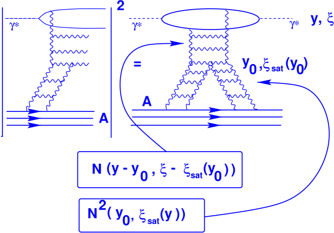
Figure 7: The diffractive production of large mass (M) ($y-y_{0}=\ln M^{2}$) in DIS.

Fig. 8 displays the DIS process in which the initial condition for the DGLAP linear evolution is fixed by the McLerran-Venugopalan model (see Ref. [1]). In other words, it is assumed that at sufficiently low energies ($y^{\prime}$ in Fig. 8), saturation at $Q^{2}_{s}(A,y^{\prime})\,\gg\,\,\Lambda^{2}$ is reached due to strong gluonic fields in a nuclear target. In this case the integral over $\xi^{\prime}$ is dominated by $\xi^{\prime}\simeq\xi_{sat}(y^{\prime})$ and the the dipole amplitude $N$ is given by

$$N(A;\xi=\ln(1/(r^{2}_{\perp}\,\Lambda^{2}),y-y^{\prime}=\ln(x^{\prime}/x))\,\,\approx\,\,e^{2\,\sqrt{\bar{\alpha}_{s}\,(\xi\,-\,\xi_{sat}(y^{\prime})(y-y^{\prime})}\,\,+\,\,\xi_{sat}(y^{\prime})\,-\,\xi}\,\,.$$ (6.30)

Since $\xi_{sat}(y^{\prime})\,\approx\,\xi_{A}$ in the initial condition for the saturation scale, the following expression is obtained:

$$\xi_{sat}(y)\,=\,4\,\bar{\alpha}_{s}\,(y-y^{\prime})\,\,+\,\,\xi_{sat}(y^{\prime})=4\,\bar{\alpha}_{s}\,(y-y^{\prime})\,\,+\,\,\xi_{A}\,\,.$$ (6.31)

The saturation scale defined in Eq. (6.31) is proportional to $A^{\frac{1}{3}}$ in a contrast to Eq. (6.22). A natural question arises: what is wrong with the first approach? Eq. (6.21) satisfies all correct initial conditions at short distances. In the integration over $\xi^{\prime}$ the main contribution comes from the upper limit of the integration $\xi^{\prime}\approx\xi_{sat}$. The integral over $\xi^{\prime}$ in the saturation region looks as follows:

$$\int^{\xi_{sat}}\,d\xi^{\prime}\,e^{\xi^{\prime}}\,\,\rightarrow\,\,e^{\xi_{sat}}.$$

For $\xi^{\prime}\,>\,\xi_{sat}$ the integral is $\int_{\xi_{sat}}\,d\xi^{\prime}\,\,e^{-\xi^{\prime}}$. This simple form of the integral is valid in the region $Q^{2}\,>\,Q^{4}_{s}/\Lambda^{2}$. This contribution is small but the estimates in the beginning of this section show that at sufficiently short distances defined by Eq. (6.22) even such a small contribution may reach so large values that we have a dense system of partons.

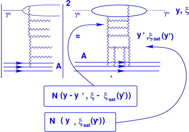
Figure 8: The total cross section for DIS with initial conditions from the McLerran-Venugopalan model.

Actually, Eq. (6.21) is

$$N(A;\xi=\ln(1/(r^{2}_{\perp}\,\Lambda^{2}),y-y_{0}=\ln(x_{0}/x))\,\,=r^{2}_{\perp}\,A\,xG(x,\frac{4}{r^{2}_{\perp}})/\pi R^{2}_{A}$$ (6.32)

in usual notations with $xG$ being in double log approximation of pQCD. Eq. (6.32) is correct at least at very short distances.

Within the same notations Eq. (6.30) looks differently

$$N(A;\xi=\ln(1/(r^{2}_{\perp}\,\Lambda^{2})),y-y_{0}=\ln(x_{0}/x))\,\,=r^{2}_{\perp}\,A\,xG(x,\frac{4}{r^{2}_{\perp}\,Q^{2}_{s}(A;y^{\prime})})/\pi R^{2}_{A}\,.$$ (6.33)

As we discussed (see Ref. [22] for more details) the geometrical scaling behavior of Eq. (6.33) is preserved till $r^{2}_{\perp}\,\approx 4\Lambda^{2}/(A^{\frac{1}{3}}\,Q^{4}_{s}(y^{\prime}))$. For shorter distances we expect the regime discussed in the beginning of this section to take place with Eq. (6.32) being correct. This should happen at $Q^{2}>Q^{4}_{sat}/(A^{\frac{1}{3}}\Lambda^{2})$ and at $x\rightarrow 0$. Unfortunately all experimentally accecible values of $x$ are not small enough for Eq. (6.21) to be seen in a nearest future.

To evaluate a typical scale of distances involved we recall that the first RHIC data are likely to reveal $Q^{2}_{s}(\mbox{Gold},x=10^{-2})\,\,\approx\,\,2\,\,GeV^{2}$ [25]. Therefore, the regime with $Q^{2}_{s}\,\propto\,A^{\frac{2}{3}}$ is expected to start at $r^{2}_{\perp}\,<\,0.01\,GeV^{-2}=4\,10^{-4}fm^{2}$. As can be seen in Fig. 1, at so short distances and at $x=10^{-2}-10^{-6}$ the diffraction amplitude is far away from the saturation region.

7 Conclusions

The non-linear evolution equation (1.5) is solved numerically for six real nuclear targets $Ne_{20}$, $Ca_{40}$, $Zn_{70}$, $Mo_{100}$, $Nd_{150}$, and $Au_{197}$. The obtained solutions display the very same pattern as in the case of proton target [16]. These solutions are used to study the $A$-dependence of single diffractive dissociation.

The saturation scale $Q_{s,\,A}^{D}$ is estimated. The fit to the parameterization $Q_{s}^{D}(A,x,x_{0})\,\sim\,A^{p}\,x^{-\lambda}\,$ reveals powers $p$ and $\lambda$. The results on $\lambda$ coincide with the corresponding power obtained for the proton case [16] while the $A$-dependence is the same as found for the saturation scale $Q_{s,\,A}$ - saturation scale obtained in total production [12]. The function $Q_{s,\,A}^{D}$ is found to be almost independent on $x_{0}$.

The geometrical scaling with respect to $x$ is well established for all nuclei considered. The scaling holds within a few percent accuracy and in the whole kinematic region investigated. As a consequence, inclusive diffractive production off nuclei is predicted to possess the scaling both with respect to $x$ and $A$. Like for a proton target the scaling phenomena with respect to $x_{0}$ set in at $x\ll x_{0}$ but is violated at $x\sim x_{0}$.

The $A$ and $x_{0}$ dependences of the determined saturation scale can be given a theoretical explanation. However, the numerically found $x$ dependence of the scale is weaker compared to the theoretical estimates.

The ratio $\sigma^{diff}/\sigma^{tot}$ was examined on a basis of the solutions obtained. At $x\simeq 10^{-4}$ a significant shadowing is expected of the order 25% and it is larger for heavy nuclei. The fact that this ratio turns out to be very close to the estimates based on the Glauber-Mueller formula [21] shows that the latter can be used as a simple approach for first estimates of possible collective effects in the saturation region of high parton density QCD.

Acnowledgements: The authors wish to thank the DESY and Hamburg University Theory Groups for their hospitality and creative atmosphere during several stages of this work. Our special thanks go to Asher Gotsman, Uri Maor and Eran Naftali for very stimulating discussion on the subject of this paper.

Part of this work done by M.L. was performed in the Technion. M.L. is very grateful to Physics Department of the Technion and especially to the members of the High Energy Group for warmness and creative atmosphere.

This research was supported in part by the BSF grant $\#$ 9800276, by the GIF grant $\#$ I-620-22.14/1999 and by Israeli Science Foundation, founded by the Israeli Academy of Science and Humanities.

References

- [1] L. V. Gribov, E. M. Levin, and M. G. Ryskin, Nucl. Phys. B 188 (1981) 555, Phys. Rep. 100 (1983) 1; A. H. Mueller and J. Qiu, Nucl. Phys. B 268 (1986) 427; L. McLerran and R. Venugopalan, Phys. Rev. D 49 (1994) 2233, 3352; D 50 (1994) 2225, D 53 (1996) 458, D 59 (1999) 094002; E. Levin and M.G. Ryskin, Phys. Rep. 189 (1990) 267; J. C. Collins and J. Kwiecinski, Nucl. Phys. B 335 (1990) 89; J. Bartels, J. Blumlein, and G. Shuler, Z. Phys. C 50 (1991) 91; E. Laenen and E. Levin, Ann. Rev. Nucl. Part. Sci. 44 (1994) 199 and references therein; Yu. Kovchegov, Phys. Rev. D 54 (1996) 5463, D 55 (1997) 5445, D 61 (2000) 074018; A. L. Ayala, M. B. Gay Ducati, and E. M. Levin, Nucl. Phys. B 493 (1997) 305, B 510 (1998) 355 A. H. Mueller, Nucl. Phys. B 572 (2000) 227, B 558 (1999) 285; J. Jalilian-Marian, A. Kovner, L. McLerran, and H. Weigert, Phys. Rev. D 55 (1997) 5414; J. Jalilian-Marian, A. Kovner, and H. Weigert, Phys. Rev. D 59 (1999) 014015; J. Jalilian-Marian, A. Kovner, A. Leonidov, and H. Weigert, Phys. Rev. D 59 (1999) 034007, Erratum-ibid. Phys. Rev. D 59 (1999) 099903; A. Kovner, J.Guilherme Milhano, and H. Weigert, Phys. Rev. D 62 (2000) 114005; H. Weigert, Nucl. Phys. A 703 (2002) 823.
- [2] Yu. Kovchegov, Phys. Rev. D 61 (2000) 074018; E. Levin and K. Tuchin, Nucl. Phys. B 573 (2000) 833; A 691 (2001) 779; E. Ferreiro, E. Iancu, K. Itakura and L. McLerran, hep-ph/0206241, Nucl. Phys. A 703 (2002) 489; E. Iancu, A.Leonidov and L. McLerran, Nucl. Phys. A 692 (2001) 583, Phys. Lett. B 510 (2001) 133.
- [3] Yu. Kovchegov and L. McLerran, Phys. Rev. D 60, 054025 (1999).
- [4] V.A. Abramovski, V.N. Gribov and O.V. Kancheli, Sov. J. Nucl. Phys. 18 (1974) 308; J. Bartels and M.G. Ryskin, Z.Phys. C 76 (1997 ) 241, hep-ph/9612226 and references therein.
- [5] A. H. Mueller, Nucl. Phys. B 415 (1994) 373.
- [6] A. H. Mueller, Nucl. Phys. B 335 (1990) 115.
- [7] N. N. Nikolaev and B. G. Zakharov, Z. Phys. C 49 (1991) 607; E. M. Levin, A. D. Martin, M. G. Ryskin, and T. Teubner, Z. Phys. C 74 (1997) 671.
- [8] Ia. Balitsky, Nucl.Phys. B 463 (1996) 99.
- [9] Yu. Kovchegov, Phys. Rev. D 60 (2000) 034008.
- [10] M. Braun, Eur. Phys. J. C 16 (2000) 337; N. Armesto and M. Braun, Eur. Phys. J. C 20 (2001) 517; K. Golec-Biernat, L. Motyka, and A. M. Stasto, Phys. Rev. D 65 (2002) 074037.
- [11] M. Lublinsky, E. Gotsman, E. Levin, and U. Maor, Nucl. Phys. A 696 (2001) 851.
- [12] E. Levin and M. Lublinsky, Nucl. Phys. A 696 (2001) 833.
- [13] Yu. Kovchegov and E. Levin, Nucl. Phys. B 577 (2000) 221.
- [14] A. Kovner and U. A. Wiedemann, Phys. Rev. D 64 (2001) 114002.
- [15] ZEUS Collaboration, J. Breitweg et al., Eur. Phys. J. C 6 (1999) 43; H1 Collaboration, C. Adloff et al., Z. Phys. C 76 (1997) 613.
- [16] E. Levin and M. Lublinsky, Eur. Phys. J. C 22 (2002) 647.
- [17] E. Levin and M. Lublinsky, Phys. Lett. B 521 (2001) 233.
- [18] C. W. De Jagier, H. De. Vries, and C. De Vries, Atomic Data and Nuclear Data Tables Vol. 14 No 5, 6 (1974) 479.
- [19] K. Golec-Biernat, J. Kwiecinski, and A. M. Stasto, Phys. Rev. Lett. 86 (2001) 596.
- [20] M. Lublinsky, Eur. Phys. J. C 21 (2001) 513.
- [21] E. Gotsman, E. Levin, M. Lublinsky, U. Maor, and K. Tuchin, Nucl. Phys. A 697 (2002) 521; Phys. Lett. B 492 (2000) 47; N. N. Nikolaev, B. G. Zakharov, and V. R. Zoller, Z. Phys. A 351 (1995) 435.
- [22] E. Iancu, K. Itakura and L. McLerran, hep-ph/0203137.
- [23] E. Levin and K. Tuchin, Nucl. Phys. A 693 (2001) 787
- [24] E. Levin and M. Wusthoff, Phys. Rev. D 50 (1994) 4306 and references thertein.
- [25] D. Kharzeev and M. Nardi, Phys. Lett. B 507 (2001) 121; D. Kharzeev and E. Levin, Phys. Lett. B 523 (2001) 79; D. Kharzeev, E. Levin and M. Nardi, hep-ph/0111315.