Supersymmetric Electroweak Corrections to Heavier Top Squark Decay into Lighter Top Squark and Neutral Higgs Boson

Qiang Li, Li Gang Jin and Chong Sheng Li

Department of Physics, Peking University, Beijing 100871, People’s Republic of China

ABSTRACT

We calculate the Yukawa corrections of order ${\cal O}(\alpha_{ew}m_{t(b)}^{2}/m_{W}^{2})$, ${\cal O}(\alpha_{ew}m_{t(b)}^{3}/m_{W}^{3})$ and ${\cal O}(\alpha_{ew}m_{t(b)}^{4}/m_{W}^{4})$ to the widths of the decays $\tilde{t}_{2}\rightarrow\tilde{t}_{1}$+$(h^{0},H^{0},A^{0})$ in the Minimal Supersymmetric Standard Model, and perform a detailed numerical analysis. We also compare the results with the ones presented in an earlier literature, where the ${\cal O}(\alpha_{s})$ SUSY-QCD corrections to the same three decay processes have been calculated. Our numerical results show that for the decays $\tilde{t}_{2}\rightarrow\tilde{t}_{1}$+$h^{0}$ , $\tilde{t}_{2}\rightarrow\tilde{t}_{1}$+$H^{0}$, the Yukawa corrections are significant in most of the parameter range, which can reach a few ten percent, and for the decay $\tilde{t}_{2}\rightarrow\tilde{t}_{1}$+$A^{0}$, the Yukawa corrections are relatively smaller, which are only a few percent. The numerical calculations also show that using the running quark masses and the running trilinear coupling $A_{t}$ , which include the QCD, SUSY-QCD, SUSY-Electroweak effects and resume all high order ($\tan\beta$)-enhanced effects, can vastly improve the convergence of the perturbation expansion. We also discuss the effects of the running of the higgsino mass parameter $\mu$ on the corrections, and find that they are significant, too, especially for large $\tan\beta$.

PACS number(s): 14.80.Cp; 14.80.Ly; 12.38.Bx

1 Introduction

Incorporation of supersymmetry is one of the most attractive and promising possibilities for new physics beyond the Standard Model (SM)[1, 2], and the Minimal Supersymmetric Standard Model (MSSM) is a popular candidate for new physics in this way. In the MSSM there are many new particles. For example, every quark has two spin zero partners called squarks $\tilde{q}_{L}$ and $\tilde{q}_{R}$, one for each chirality eigenstate, which mix to form the mass eigenstates $\tilde{q}_{1}$ and $\tilde{q}_{2}$. For the third generation quarks, due to large Yukawa couplings, there may be large mass differences between the lighter mass eigenstate and the heavier one, which implies in general a very complex decay pattern of the heavier state.

As we know, the next generation of colliders, such as the Large Hadron Collider (LHC), the upgraded Tevatron, $e^{+}e^{-}$ linear colliders, and $\mu^{+}\mu^{-}$ collider will push the discovery reach for supersymmetric (SUSY) paticles with masses up to 2.5 TeV[3, 4] and allow for precise measurement of the MSSM parameters. Thus a more accurate calculations of the deacy mechanisms beyond the tree level are necessary. The dominate decay modes of the heavier squarks are shown as below:

$$\tilde{t}_{i}\rightarrow t\tilde{x}_{k}^{0},b\tilde{x}_{k}^{+};\tilde{b}_{i}\rightarrow b\tilde{x}_{k}^{0},t\tilde{x}_{k}^{+};\ \ \tilde{t}_{i}\rightarrow t\tilde{g};\tilde{b}_{i}\rightarrow b\tilde{g};$$

$$\tilde{t}_{2}\rightarrow\tilde{t}_{1}Z^{0};\tilde{t}_{i}\rightarrow\tilde{b}_{j}W^{+};\ \ \tilde{b}_{2}\rightarrow\tilde{b}_{1}Z^{0};\tilde{b}_{i}\rightarrow\tilde{t}_{j}W^{-};$$

$$\tilde{b}_{i}\rightarrow\tilde{t}_{j}H^{-};\tilde{t}_{i}\rightarrow\tilde{b}_{j}H^{+};\ \ \ \tilde{t}_{2}\rightarrow\tilde{t}_{1}(h^{0},H^{0},A^{0}).$$

All these squark decays have been extensively discussed at the tree-level[5, 6, 7]. Up to now, one-loop QCD and supersymmetric (SUSY) QCD corrections to above decay channels have been calculated too [6, 8, 9], while the Yukawa corrections and the full electroweak one-loop radiative corrections to the squark decays into quarks plus charginos/neutralinos were given in Ref.[10] and Ref.[11], respectively. Also the Yukawa corrections to the squark decays into quarks plus gluinos were given in Refs.[12, 13], and the Yukawa corrections to the heavier squark decays into lighter squarks plus vetor bosons were given in Ref.[14]. Recently, the Yukawa corrections to the bottom squark decays into lighter top squarks plus charged Higgs bosons has been presented in Ref.[15]. So only the electroweak radiative corrections to the heavier top squark decays into lighter top squarks plus neutral Higgs bosons have not been calculated yet, including the Yukawa corrections to these processes.

In this paper, we present the calculations of the Yukawa corrections of order ${\cal O}(\alpha_{ew}m_{t(b)}^{2}/m_{W}^{2})$, ${\cal O}(\alpha_{ew}m_{t(b)}^{3}/m_{W}^{3})$, and ${\cal O}(\alpha_{ew}m_{t(b)}^{4}/m_{W}^{4})$ to the widths of the heavier top squark decays into lighter top squarks plus neutral Higgs bosons, i.e.the decays $\tilde{t}_{2}\rightarrow\tilde{t}_{1}+(h^{0},H^{0},A^{0})$. These corrections are mainly induced by the Yukawa couplings from Higgs-quark-quark couplings, Higgs-squark-squark couplings, Higgs-Higgs-squark-squark couplings, chargino(neutralino)-quark-squark couplings, and squark-squark-squark-squark couplings. As shown in Ref.[16], the Higgs-Squark-Squark couplings receive large radiative corrections, which can make the perturbation calculation of the relevant Squark or Higgs boson decay widths quite unreliable in some region of the parameter space. When the correction term is negative, the corrected width can even become negative, which clearly makes no sense. In order to solve this problem, we use the running quark masses and the running trilinear coupling $A_{t}$ [16], and vastly improve the convergence of the perturbation expansion. We also discuss the effects of the running of the higgsino mass parameter $\mu$ on the corrections, and find that they are significant, too, especially for large $\tan\beta$.

2 Notation and tree-level result

In order to make this paper self-contained, we first summarize our notation and present the relevant interaction Lagrangians of the MSSM and the tree-level decay rates for $\tilde{t}_{2}\rightarrow\tilde{t}_{1}+(h^{0},H^{0},A^{0})$.

The current eigenstates $\tilde{q}_{L}$ and $\tilde{q}_{R}$ are related to the mass eigenstates $\tilde{q}_{1}$ and $\tilde{q}_{2}$ by

$$\left(\begin{array}[]{c}\tilde{q}_{1}\\ \tilde{q}_{2}\end{array}\right)=R^{\tilde{q}}\left(\begin{array}[]{c}\tilde{q}_{L}\\ \tilde{q}_{R}\end{array}\right),\ \ \ \ \ R^{\tilde{q}}=\left(\begin{array}[]{cc}\cos\theta_{\tilde{q}}&\sin\theta_{\tilde{q}}\\ -\sin\theta_{\tilde{q}}&\cos\theta_{\tilde{q}}\end{array}\right)$$ (1)

with $0\leq\theta_{\tilde{q}}<\pi$ by convention. Correspondingly, the mass eigenvalues $m_{\tilde{q}_{1}}$ and $m_{\tilde{q}_{2}}$ (with $m_{\tilde{q}_{1}}\leq m_{\tilde{q}_{2}}$) are given by

$$\left(\begin{array}[]{cc}m_{\tilde{q}_{1}}^{2}&0\\ 0&m_{\tilde{q}_{2}}^{2}\end{array}\right)=R^{\tilde{q}}M_{\tilde{q}}^{2}(R^{\tilde{q}})^{\dagger},\ \ \ \ \ M_{\tilde{q}}^{2}=\left(\begin{array}[]{cc}m_{\tilde{q}_{L}}^{2}&a_{q}m_{q}\\ a_{q}m_{q}&m_{\tilde{q}_{R}}^{2}\end{array}\right)$$ (6)

with

$$m^{2}_{\tilde{q}_{L}} = M^{2}_{\tilde{Q}}+m_{q}^{2}+m_{Z}^{2}\cos 2\beta(I_{3L}^{q}-e_{q}\sin^{2}\theta_{W}),$$ (7)

$$m^{2}_{\tilde{q}_{R}} = M^{2}_{\{\tilde{U},\tilde{D}\}}+m_{q}^{2}+m_{Z}^{2}\cos 2\beta e_{q}\sin^{2}\theta_{W},$$ (8)

$$a_{q} = A_{q}-\mu\{\cot\beta,\tan\beta\}$$ (9)

for {up, down} type squarks. Here $M_{\tilde{q}}^{2}$ is the squark mass matrix. $M_{\tilde{Q},\tilde{U},\tilde{D}}$ and $A_{t,b}$ are soft SUSY-breaking parameters and $\mu$ is the higgsino mass parameter . $I_{3L}^{q}$ and $e_{q}$ are the third component of the weak isospin and the electric charge of the quark $q$, respectively.

Defining $H_{k}=(h^{0},H^{0},A^{0},G^{0},H^{\pm},G^{\pm})$ ($k$=1,…,6), one can write the relevant lagrangian density in the ($\tilde{q}_{1},\tilde{q}_{2}$) basis as following form ($i,j$=1,2; $\alpha$ and $\beta$ are flavor indices):

$${\cal L}_{\rm relevant}=H_{k}\bar{q}^{\beta}(a_{k}^{\alpha}P_{L}+b_{k}^{\alpha}P_{R})q^{\alpha}+(G^{\tilde{\alpha}}_{k})_{ij}H_{k}\tilde{q}_{j}^{\beta\ast}\tilde{q}^{\alpha}_{i}+g\bar{q}(a_{ik}^{\tilde{q}}P_{R}+b_{ik}^{\tilde{q}})\tilde{\chi}^{0}_{k}\tilde{q}_{i}$$

$$\hskip 42.67912pt+g\bar{t}(l_{ik}^{\tilde{b}}P_{R}+k_{ik}^{\tilde{b}}P_{L})\tilde{\chi}^{+}_{k}\tilde{b}_{i}+g\bar{b}(l_{ik}^{\tilde{t}}P_{R}+k_{ik}^{\tilde{t}}P_{L})\tilde{\chi}_{k}^{+c}\tilde{t}_{i}$$

$$\hskip 42.67912pt+(G^{\tilde{\alpha}}_{lk})_{ij}H_{l}H_{k}\tilde{q}_{j}^{\beta\ast}\tilde{q}^{\alpha}_{i}+h.c.,$$ (10)

with

$$(G^{\tilde{\alpha}}_{lk})_{ij}=[R^{\tilde{\alpha}}\hat{G}_{lk}^{\tilde{\alpha}}(R^{\tilde{\beta}})^{T}]_{ij}\hskip 8.5359pt(l,k=1,...,6)$$ (11)

$$(G^{\tilde{\alpha}}_{k})_{ij}=[R^{\tilde{\alpha}}\hat{G}_{k}^{\tilde{\alpha}}(R^{\tilde{\beta}})^{T}]_{ij}\hskip 8.5359pt(k=1,...,6)$$ (12)

where $\hat{G}^{\tilde{\alpha}}_{k}$ and $\hat{G}^{\tilde{\alpha}}_{lk}$ are the couplings in the ($\tilde{q}_{L},\tilde{q}_{R}$) basis , and their explicit forms are shown in Appendix A. The notations $a_{k}^{\alpha}$, $b_{k}^{\alpha}$ (k=1,…,6), and $a_{ik}^{\tilde{q}}$, $b_{ik}^{\tilde{q}}$ (k=1,…,4), and $l_{ik}^{\tilde{q}}$, $k_{ik}^{\tilde{q}}$ (k=1,2) used in Eq.(2) are defined also in Appendix A.

The tree-level amplitudes of the three decay processes, as shown in Fig.1(a), are given by

$$M^{(0)}_{1}=i[R^{\tilde{t}}\left(\begin{array}[]{cc}-\sqrt{2}m_{t}h_{t}\cos\alpha+\frac{gm_{z}\sin(\alpha+\beta)}{c_{W}}C_{tL}&\frac{-h_{t}}{\sqrt{2}}(A_{t}\cos\alpha+\mu\sin\alpha)\\ \frac{-h_{t}}{\sqrt{2}}(A_{t}\cos\alpha+\mu\sin\alpha)&-\sqrt{2}m_{t}h_{t}\cos\alpha+\frac{gm_{z}\sin(\alpha+\beta)}{c_{W}}C_{tR}\end{array}\right)(R^{\tilde{t}})^{T}]_{21}$$ (15)

for $\tilde{t}_{2}\rightarrow\tilde{t}_{1}h^{0}$,

$$M^{(0)}_{2}=i[R^{\tilde{t}}\left(\begin{array}[]{cc}-\sqrt{2}m_{t}h_{t}\sin\alpha-\frac{gm_{z}\cos(\alpha+\beta)}{c_{W}}C_{tL}&\frac{-h_{t}}{\sqrt{2}}(A_{t}\sin\alpha-\mu\cos\alpha)\\ \frac{-h_{t}}{\sqrt{2}}(A_{t}\sin\alpha-\mu\cos\alpha)&-\sqrt{2}m_{t}h_{t}\sin\alpha-\frac{gm_{z}\cos(\alpha+\beta)}{c_{W}}C_{tR}\end{array}\right)(R^{\tilde{t}})^{T}]_{21}$$ (18)

for $\tilde{t}_{2}\rightarrow\tilde{t}_{1}H^{0}$, and

$$\noindent M^{(0)}_{3}=\frac{gm_{t}}{2m_{W}}[R^{\tilde{t}}\left(\begin{array}[]{cc}0&A_{t}\cot\beta+\mu\\ -A_{t}\cot\beta-\mu&0\end{array}\right)(R^{\tilde{t}})^{T}]_{21}$$ (21)

for $\tilde{t}_{2}\rightarrow\tilde{t}_{1}A^{0}$. Here $h_{t}=\frac{gm_{t}}{\sqrt{2}m_{W}\sin\beta}$, $h_{b}=\frac{gm_{b}}{\sqrt{2}m_{W}\cos\beta}$, $C_{tL}=I_{3L}^{t}-e_{t}s^{2}_{W}$, $C_{tR}=e_{t}s^{2}_{w}$, $s_{W}=\sin\theta_{w}$, and $c_{w}=\cos\theta_{w}$. $I_{3L}^{t}=\frac{1}{2}$ and $e_{t}=\frac{2}{3}$ for the top squark, $I_{3L}^{b}=-\frac{1}{2}$ and $e_{b}=-\frac{1}{3}$ for the bottom squark. The tree-level decay width is thus given by

$$\Gamma^{(0)}_{s}=\frac{|M^{(0)}_{s}|^{2}\lambda^{1/2}(m_{\tilde{t}_{2}}^{2},m_{\tilde{t}_{1}}^{2},m_{H^{0}_{s}}^{2})}{16\pi m_{\tilde{t}_{2}}^{3}},$$ (22)

where $\lambda(x,y,z)=(x-y-z)^{2}-4yz$ and s=(1,2,3) corresponds to the decay into $(h^{0},H^{0},A^{0})$, respectively.

3 Yukawa corrections

The Feynman diagrams contributing to the Yukawa corrections to $\tilde{t}_{2}\rightarrow\tilde{t}_{1}H^{0}_{i}$ are shown in Figs.1(b)–(f) and Fig.2. We carried out the calculation in the t’Hooft-Feynman gauge and used the dimensional reduction, which preserves supersymmetry, for regularization of the ultraviolet divergences in the virtual loop corrections using the on-mass-shell renormalization scheme[17], in which the fine-structure constant $\alpha_{ew}$ and physical masses are chosen to be the renormalized parameters, and finite parts of the counterterms are fixed by the renormalization conditions. The coupling constant $g$ is related to the input parameters $e$, $m_{W}$ and $m_{Z}$ via $g^{2}=e^{2}/s_{w}^{2}$ and $s_{w}^{2}=1-m_{W}^{2}/m_{Z}^{2}$. As for the renormalization of the parameters in the Higgs sector and the squark sector, it will be described in detail below.

The relevant renormalization constants are defined as

$$m_{W0}^{2}=m_{W}^{2}+\delta m_{W}^{2},\hskip 14.22636ptm_{Z0}^{2}=m_{Z}^{2}+\delta m_{Z}^{2},$$

$$m_{q0}=m_{q}+\delta m_{q},\hskip 28.45274ptm_{\tilde{q}_{i}0}^{2}=m_{\tilde{q}_{i}}^{2}+\delta m_{\tilde{q}_{i}}^{2},$$

$$A_{q0}=A_{q}+\delta A_{q},\hskip 34.14322pt\mu_{0}=\mu+\delta\mu,$$

$$\theta_{\tilde{q}0}=\theta_{\tilde{q}}+\delta\theta_{\tilde{q}},\hskip 42.67912pt\tan\beta_{0}=(1+\delta Z_{\beta})\tan\beta,$$

$$\sin\alpha_{0}=(1+\delta Z_{\alpha})\sin\alpha,$$

$$\tilde{q}_{i0}=(1+\delta Z^{\tilde{q}}_{i})^{1/2}+\delta Z^{\tilde{q}}_{ij}\tilde{q}_{j},$$

$$H^{0}_{0}=(1+\delta Z_{H^{0}})^{1/2}H^{0}+\delta Z_{H^{0}h^{0}}h^{0},$$

$$h^{0}_{0}=(1+\delta Z_{h^{0}})^{1/2}h^{0}+\delta Z_{h^{0}H^{0}}H^{0},$$

$$G_{0}^{-}=(1+\delta Z_{G^{-}})^{1/2}G^{-}+\delta Z_{GH}H^{-},$$

$$A_{0}^{0}=(1+\delta Z_{A^{0}})^{1/2}A^{0}$$ (23)

with $q=t,b$. Here we introduce the mixing of $H^{-}$ and $G^{-}$[18].

Taking into account the Yukawa corrections, the renormalized amplitude for $\tilde{t}_{2}\rightarrow\tilde{t}_{1}H_{s}^{0}$ is given by

$$M^{ren}_{s}=M^{(0)}_{s}+\delta M^{(v)}_{s}+\delta M^{(c)}_{s},$$ (24)

where $\delta M^{(v)}_{s}$ and $\delta M^{(c)}_{s}$ are the vertex corrections and the counterterms, respectively.

The calculations of the vertex corrections from Fig.1(b)-1(f) result in

$$\delta M^{(v)}_{s=1,2,3}=\frac{i}{16\pi^{2}}\sum_{k=1}^{6}\sum_{j}(G_{sk}^{\tilde{t}})_{2j}(G_{k}^{\tilde{q}})_{j1}B_{0}(m^{2}_{\tilde{t}_{1}},m_{H_{k}^{0}},m_{\tilde{q}_{j}})$$

$$\hskip 45.52458pt-\frac{i}{16\pi^{2}}\sum_{k=1}^{6}\sum_{ij}(G_{s}^{\tilde{t}})_{ij}(G_{k}^{\tilde{t}})_{2i}(G_{k}^{\tilde{q}})_{j1}C_{0}(p_{\tilde{t}_{1}},p_{H_{s}^{0}},m_{H_{k}^{0}},m_{\tilde{q}_{j}},m_{\tilde{q}_{i}})$$

$$\hskip 45.52458pt+\frac{i}{16\pi^{2}}\sum_{k=1}^{6}\sum_{j}(G_{sk}^{\tilde{t}})_{j1}(G_{k}^{\tilde{q}})_{2j}B_{0}(m^{2}_{\tilde{t}_{2}},m_{H_{k}^{0}},m_{\tilde{q}_{j}})$$

$$\hskip 45.52458pt-\frac{i}{16\pi^{2}}\sum_{ij}\sin\theta_{\tilde{t}}\cos\theta_{\tilde{t}}(h_{t}^{2}R^{\tilde{b}}_{i1}R^{\tilde{b}}_{j1}-h_{b}^{2}R^{\tilde{b}}_{i2}R^{\tilde{b}}_{j2})(G_{s}^{\tilde{b}})_{ij}B_{0}(m^{2}_{H_{s}^{0}},m_{\tilde{b}_{j}},m_{\tilde{b}_{i}})$$

$$\hskip 45.52458pt-\frac{ih_{t}^{2}}{16\pi^{2}}\{\hskip 4.26773pt[3(\sin^{4}\theta_{\tilde{t}}+\cos^{4}\theta_{\tilde{t}})-2\sin^{2}\theta_{\tilde{t}}\cos^{2}\theta_{\tilde{t}}](G_{s}^{\tilde{t}})_{21}B_{0}(m^{2}_{H_{s}^{0}},m_{\tilde{t}_{1}},m_{\tilde{t}_{2}})$$

$$\hskip 71.13188pt-8\sin^{2}\theta_{\tilde{t}}\cos^{2}\theta_{\tilde{t}}(G_{s}^{\tilde{t}})_{12}B_{0}(m^{2}_{H_{s}^{0}},m_{\tilde{t}_{2}},m_{\tilde{t}_{1}})$$

$$\hskip 71.13188pt+4\sin\theta_{\tilde{t}}\cos\theta_{\tilde{t}}\cos 2\theta_{\tilde{t}}(G_{s}^{\tilde{t}})_{11}B_{0}(m^{2}_{H_{s}^{0}},m_{\tilde{t}_{1}},m_{\tilde{t}_{1}})$$

$$\hskip 71.13188pt-4\sin\theta_{\tilde{t}}\cos\theta_{\tilde{t}}\cos 2\theta_{\tilde{t}}(G_{s}^{\tilde{t}})_{22}B_{0}(m^{2}_{H_{s}^{0}},m_{\tilde{t}_{2}},m_{\tilde{t}_{2}})\hskip 4.26773pt\}$$

$$\hskip 45.52458pt+F_{\chi s}.$$ (25)

where $F_{\chi s}$ is the remains, which are given by

$$\hskip 22.76228ptF_{\chi s}=-\frac{ig^{2}h_{t}\cos(\alpha-(s-1)\frac{\pi}{2})}{16\sqrt{2}\pi^{2}}\sum_{i}\{\hskip 8.5359pt[2(a_{2i}^{\tilde{t}}{a_{1i}^{\tilde{t}}}^{*}+b_{2i}^{\tilde{t}}{b_{1i}^{\tilde{t}}}^{*})m_{t}][(2m_{\tilde{t}_{1}}^{2}+p_{\tilde{t}_{1}}p_{H_{s}^{0}})C_{11}$$

$$\hskip 34.14322pt+(2p_{\tilde{t}_{1}}p_{H_{s}^{0}}+m_{H_{s}^{0}}^{2})C_{12}+2m_{\tilde{t}_{1}}^{2}C_{21}+2m_{H_{s}^{0}}^{2}C_{22}+4p_{\tilde{t}_{1}}p_{H_{s}^{0}}C_{23}+8C_{24}]$$

$$\hskip 34.14322pt+[2(a_{2i}^{\tilde{t}}{b_{1i}^{\tilde{t}}}^{*}+b_{2i}^{\tilde{t}}{a_{1i}^{\tilde{t}}}^{*})m_{{\tilde{\chi}_{i}^{0}}}][(2m_{\tilde{t}_{1}}^{2}+p_{\tilde{t}_{1}}p_{H_{s}^{0}})C_{11}+(2p_{\tilde{t}_{1}}p_{H_{s}^{0}}+m_{H_{s}^{0}}^{2})C_{12}$$

$$\hskip 34.14322pt+(m_{\tilde{t}_{1}}^{2}C_{21}+m_{H_{s}^{0}}^{2}C_{22}+2p_{\tilde{t}_{1}}p_{H_{s}^{0}}C_{23}+4C_{24}+(m_{\tilde{t}_{1}}^{2}+p_{\tilde{t}_{1}}p_{H_{s}^{0}})C_{0}+m_{t}^{2}C_{0}]$$

$$\hskip 34.14322pt\}(p_{\tilde{t}_{1}},p_{H_{s}^{0}},m_{{\tilde{\chi}_{i}^{0}}},m_{t},m_{t})$$

$$\hskip 34.14322pt+\frac{ig^{2}h_{b}\sin(\alpha-(s-1)\frac{\pi}{2})}{16\sqrt{2}\pi^{2}}\sum_{i}\{\hskip 8.5359pt[2(l_{2i}^{\tilde{t}}{l_{1i}^{\tilde{t}}}^{*}+k_{2i}^{\tilde{t}}{k_{1i}^{\tilde{t}}}^{*})m_{b}][(2m_{\tilde{t}_{1}}^{2}+p_{\tilde{t}_{1}}p_{H_{s}^{0}})C_{11}$$

$$\hskip 34.14322pt+(2p_{\tilde{t}_{1}}p_{H_{s}^{0}}+m_{H_{s}^{0}}^{2})C_{12}+2m_{\tilde{t}_{1}}^{2}C_{21}+2m_{H_{s}^{0}}^{2}C_{22}+4p_{\tilde{t}_{1}}p_{H_{s}^{0}}C_{23}+8C_{24}]$$

$$\hskip 34.14322pt+[2(l_{2i}^{\tilde{t}}{k_{1i}^{\tilde{t}}}^{*}+k_{2i}^{\tilde{t}}{l_{1i}^{\tilde{t}}}^{*})m_{{\tilde{\chi}_{i}}^{-}}][(2m_{\tilde{t}_{1}}^{2}+p_{\tilde{t}_{1}}p_{H_{s}^{0}})C_{11}+(2p_{\tilde{t}_{1}}p_{H_{s}^{0}}+m_{H_{s}^{0}}^{2})C_{12}$$

$$\hskip 34.14322pt+(m_{\tilde{t}_{1}}^{2}C_{21}+m_{H_{s}^{0}}^{2}C_{22}+2p_{\tilde{t}_{1}}p_{H_{s}^{0}}C_{23}+4C_{24}+(m_{\tilde{t}_{1}}^{2}+p_{\tilde{t}_{1}}p_{H_{s}^{0}})C_{0}+m_{b}^{2}C_{0}]$$

$$\hskip 34.14322pt\}(p_{\tilde{t}_{1}},p_{H_{s}^{0}},m_{{\tilde{\chi}_{i}}^{-}},m_{b},m_{b})$$ (26)

for s=(1,2), and

$$F_{\chi 3}=-\frac{g^{3}m_{t}\cot\beta}{32\pi^{2}m_{W}}\sum_{i}\{\hskip 8.5359pt[2(a_{2i}^{\tilde{t}}{a_{1i}^{\tilde{t}}}^{*}-b_{2i}^{\tilde{t}}{b_{1i}^{\tilde{t}}}^{*})m_{t}](m_{A^{0}}^{2}C_{12}+p_{\tilde{t}_{1}}p_{A^{0}}C_{11})$$

$$\hskip 34.14322pt+[2(a_{2i}^{\tilde{t}}{b_{1i}^{\tilde{t}}}^{*}-b_{2i}^{\tilde{t}}{a_{1i}^{\tilde{t}}}^{*})m_{{\tilde{\chi}_{i}^{0}}}][(2m_{\tilde{t}_{1}}^{2}+p_{\tilde{t}_{1}}p_{A^{0}})C_{11}+(2p_{\tilde{t}_{1}}p_{A^{0}}+m_{A^{0}}^{2})C_{12}$$

$$\hskip 34.14322pt+m_{\tilde{t}_{1}}^{2}C_{21}+m_{A^{0}}^{2}C_{22}+2p_{\tilde{t}_{1}}p_{A^{0}}C_{23}+4C_{24}+(p_{\tilde{t}_{1}}^{2}+p_{\tilde{t}_{1}}p_{A^{0}})C_{0}-m_{t}^{2}C_{0}]$$

$$\hskip 34.14322pt\}(p_{\tilde{t}_{1}},p_{A^{0}},m_{{\tilde{\chi}_{i}^{0}}},m_{t},m_{t})$$

$$\hskip 34.14322pt-\frac{ig^{3}m_{b}\tan\beta}{32\pi^{2}m_{W}}\sum_{i}\{\hskip 8.5359pt[2(l_{2i}^{\tilde{t}}{l_{1i}^{\tilde{t}}}^{*}-k_{2i}^{\tilde{t}}{k_{1i}^{\tilde{t}}}^{*})m_{b}](m_{A^{0}}^{2}C_{12}+p_{\tilde{t}_{1}}p_{A^{0}}C_{11})$$

$$\hskip 34.14322pt+[2(l_{2i}^{\tilde{t}}{k_{1i}^{\tilde{t}}}^{*}-k_{2i}^{\tilde{t}}{l_{1i}^{\tilde{t}}}^{*})m_{{\tilde{\chi}_{i}}^{-}}][(2m_{\tilde{t}_{1}}^{2}+p_{\tilde{t}_{1}}p_{A^{0}})C_{11}+(2p_{\tilde{t}_{1}}p_{A^{0}}+m_{A^{0}}^{2})C_{12}$$

$$\hskip 34.14322pt+m_{\tilde{t}_{1}}^{2}C_{21}+m_{A^{0}}^{2}C_{22}+2p_{\tilde{t}_{1}}p_{A^{0}}C_{23}+4C_{24}+(p_{\tilde{t}_{1}}^{2}+p_{\tilde{t}_{1}}p_{A^{0}})C_{0}-m_{b}^{2}C_{0}]$$

$$\hskip 34.14322pt\}(p_{\tilde{t}_{1}},p_{A^{0}},m_{{\tilde{\chi}_{i}}^{-}},m_{b},m_{b})$$ (27)

for s=3. In above expressions $B_{0}$ and $C_{i(j)}$ are two- and three-point Feynman integrals[20], respectively. For $q=t$, we have $k=1...4$. For $q=b$, we have $k=5,6$.

The counterterms can be expressed as

$$\delta M^{(c)}_{1}=i(G_{1}^{\tilde{t}})_{21}[\frac{1}{2}(\delta Z_{1}+\delta Z_{2}+\delta Z_{h^{0}})-2\tan 2\theta_{\tilde{t}}\delta\theta_{\tilde{t}}+\frac{\delta g}{g}-\frac{\delta m_{W}^{2}}{2m_{W}^{2}}-\cos^{2}\beta\delta\beta]$$

$$\hskip 42.67912pt-i\frac{gm_{t}A_{t}\cos\alpha}{2m_{W}\sin\beta}\cos 2\theta_{\tilde{t}}[\frac{A_{t}\delta m_{t}+m_{t}\delta A_{t}}{m_{t}A_{t}}+\tan^{2}\alpha\delta Z_{\alpha}]$$

$$\hskip 42.67912pt-i\frac{gm_{t}\mu\sin\alpha}{2m_{W}\sin\beta}\cos 2\theta_{\tilde{t}}[\frac{\delta\mu}{\mu}+\frac{\delta m_{t}}{m_{t}}-\delta Z_{\alpha}]$$

$$\hskip 42.67912pt+i(G_{1}^{\tilde{t}})_{11}\delta Z_{12}+i(G_{1}^{\tilde{t}})_{22}\delta Z_{21}+i(G_{2}^{\tilde{t}})_{21}\delta Z_{H^{0}h^{0}},$$ (28)

$$\delta M^{(c)}_{2}=i(G_{2}^{\tilde{t}})_{21}[\frac{1}{2}(\delta Z_{1}+\delta Z_{2}+\delta Z_{H^{0}})-2\tan 2\theta_{\tilde{t}}\delta\theta_{\tilde{t}}+\frac{\delta g}{g}-\frac{\delta m_{W}^{2}}{2m_{W}^{2}}-\cos^{2}\beta\delta\beta]$$

$$\hskip 42.67912pt-i\frac{gm_{t}A_{t}\sin\alpha}{2m_{W}\sin\beta}\cos 2\theta_{\tilde{t}}[\frac{A_{t}\delta m_{t}+m_{t}\delta A_{t}}{m_{t}A_{t}}+\delta Z_{\alpha}]$$

$$\hskip 42.67912pt+i\frac{g\mu m_{t}\cos\alpha}{2m_{W}\sin\beta}\cos 2\theta_{\tilde{t}}[\frac{\delta\mu}{\mu}+\frac{\delta m_{t}}{m_{t}}-\tan^{2}\alpha\delta Z_{\alpha}]$$

$$\hskip 42.67912pt+i(G_{2}^{\tilde{t}})_{11}\delta Z_{12}+i(G_{2}^{\tilde{t}})_{22}\delta Z_{21}+i(G_{1}^{\tilde{t}})_{21}\delta Z_{h^{0}H^{0}},$$ (29)

$$\delta M^{(c)}_{3}=i(G_{3}^{\tilde{t}})_{21}[\frac{1}{2}(\delta Z_{1}+\delta Z_{2}+\delta Z_{A^{0}})+\frac{\delta g}{g}-\frac{\delta m_{W}^{2}}{2m_{W}^{2}}]$$

$$\hskip 42.67912pt-\frac{gm_{t}A_{t}\cos\alpha}{2m_{W}}\cot\beta[\frac{\delta(m_{t}A_{t})}{m_{t}A_{t}}-\delta Z_{\beta}]-\frac{g\mu m_{t}}{2m_{W}}[\frac{\delta\mu}{\mu}+\frac{\delta m_{t}}{m_{t}}].$$ (30)

Here we consider only the counterterms from the Yukawa couplings, and the explicit expressions of some renormalization constants calculated from the self-energy diagrams in Fig.2 are given in Appendix B. Other renormalization constants are fixed as follows.

For $\delta Z_{GH}$, using the approach discussed in the two-Higgs doublet model (2HDM) in [18], we derived below its expression in the MSSM, where the version of the Higgs potential is different from one of Ref.[18]. First, the one-loop renormalized two-point function is given by

$$i\Gamma_{GH}(p^{2})=i(p^{2}-m_{H^{-}}^{2})\delta Z_{HG}+ip^{2}\delta Z_{GH}-iT_{GH}+i\Sigma_{GH}(p^{2}),$$ (31)

where $T_{GH}$ is the tadpole function, which is given by

$$T_{GH}=\frac{g}{2m_{W}}[T_{H_{2}}\sin(\alpha-\beta)+T_{H_{1}}\cos(\alpha-\beta)].$$ (32)

Next, from the on-shell renormalization condition, we obtained

$$\delta Z_{GH}=\frac{1}{m_{H^{-}}^{2}}[T_{GH}-\Sigma_{GH}(m_{H^{-}}^{2})].$$ (33)

The explicit expressions of $\Sigma_{GH}$ and the tadpole counterterms $T_{H_{k}}$ $(k=1,2)$ are given in Appendix B.

For the renormalization of the parameter $\beta$, following the analysis of Ref.[19], we fixed the renormalization constant by the requirement that the on-mass-shell $H^{+}\bar{\tau}\nu_{\tau}$ coupling remain the same form as in Eq.(3) of Ref.[19] to all orders of perturbation theory. However, with introducing the mixing of $H^{-}$ and $G^{-}$ instead of $H^{-}$ and $W^{-}$, the expression of $\delta Z_{\beta}$ is then changed to

$$\delta Z_{\beta}=\frac{1}{2}\frac{\delta m_{W}^{2}}{m_{W}^{2}}-\frac{1}{2}\frac{\delta m_{Z}^{2}}{m_{Z}^{2}}+\frac{1}{2}\frac{\delta m_{Z}^{2}-\delta m_{W}^{2}}{m_{Z}^{2}-m_{W}^{2}}-\frac{1}{2}\delta Z_{H^{+}}+\cot\beta\delta Z_{GH}.$$ (34)

For the counterterm of squark mixing angle $\theta_{\tilde{q}}$, using the same renormalized scheme as Ref.[10], one has

$$\delta\theta_{\tilde{q}}=\frac{{\rm Re}[\Sigma_{12}^{\tilde{q}}(m_{\tilde{q}_{1}}^{2})+\Sigma_{12}^{\tilde{q}}(m_{\tilde{q}_{2}}^{2})]}{2(m_{\tilde{q}_{1}}^{2}-m_{\tilde{q}_{2}}^{2})},$$ (35)

where the explicit expressions of the $\Sigma_{ij}$ functions arising from the self-energy diagrams due to the Yukawa couplings are given in the Appendix B.

For the renormalization of soft SUSY-breaking parameter $A_{q}$, we fixed its counterterm by keeping the tree-level relation of $A_{q}$, $m_{\tilde{q}_{i}}$ and $\theta_{\tilde{q}}$ [21], and get the expression as following:

$$\delta A_{q}=\frac{m_{\tilde{q}_{1}}^{2}-m_{\tilde{q}_{2}}^{2}}{2m_{q}}(2\cos{2\theta_{\tilde{q}}}\delta\theta_{\tilde{q}}-\sin{2\theta_{\tilde{q}}}\frac{\delta m_{q}}{m_{q}})+\frac{\sin{2\theta_{\tilde{q}}}}{2m_{q}}(\delta m_{\tilde{q}_{1}}^{2}-\delta m_{\tilde{q}_{2}}^{2})$$

$$\hskip 36.98866pt+\{\cot\beta,\tan\beta\}\delta\mu+\delta\{\cot\beta,\tan\beta\}\mu.$$ (36)

As for the parameter $\mu$, there are several schemes[11, 22, 23] to fix its counterterm, and here we use the on-shell renormalization scheme in Ref.[23], which gives

$$\delta\mu=\sum_{k=1}^{2}[m_{\tilde{\chi}_{k}^{+}}(\delta U_{k2}V_{k2}+U_{k2}\delta V_{k2})+\delta m_{\tilde{\chi}_{k}^{+}}U_{k2}V_{k2}],$$ (37)

where $(U,V)$ are the two $2\times 2$ matrices diagonalizing the chargino mass matrix, and their counterterms $(\delta U,\delta V)$ are given by

$$\delta U=\frac{1}{4}(\delta Z_{R}-\delta Z_{R}^{T})U,$$ (38)

$$\delta V=\frac{1}{4}(\delta Z_{L}-\delta Z_{L}^{T})V.$$ (39)

The mass shifts $\delta m_{\tilde{\chi}_{k}^{+}}$ and the off-diagonal wave function renormalization constants $\delta Z_{R(L)}$ can be written as

$$\delta m_{\tilde{\chi}_{k}^{+}}=\frac{1}{2}{\rm Re}[m_{\tilde{\chi}_{k}^{+}}(\Pi_{kk}^{L}(m_{\tilde{\chi}_{k}^{+}}^{2})+\Pi_{kk}^{R}(m_{\tilde{\chi}_{k}^{+}}^{2}))+\Pi_{kk}^{S,L}(m_{\tilde{\chi}_{k}^{+}}^{2})+\Pi_{kk}^{S,R}(m_{\tilde{\chi}_{k}^{+}}^{2})],$$ (40)

$$(\delta Z_{R})_{ij}=\frac{2}{m_{\tilde{\chi}_{i}^{+}}^{2}-m_{\tilde{\chi}_{j}^{+}}^{2}}{\rm Re}[\Pi_{ij}^{R}(m_{\tilde{\chi}_{j}^{+}}^{2})m_{\tilde{\chi}_{j}^{+}}^{2}+\Pi_{ij}^{L}(m_{\tilde{\chi}_{j}^{+}}^{2})m_{\tilde{\chi}_{i}^{+}}m_{\tilde{\chi}_{j}^{+}}$$

$$\hskip 170.71652pt+\Pi_{ij}^{S,R}(m_{\tilde{\chi}_{j}^{+}}^{2})m_{\tilde{\chi}_{i}^{+}}+\Pi_{ij}^{S,L}(m_{\tilde{\chi}_{j}^{+}}^{2})m_{\tilde{\chi}_{j}^{+}}],$$ (41)

$$(\delta Z_{L})_{ij}=(\delta Z_{R})_{ij}\ \ (L\leftrightarrow R).$$ (42)

The explicit expressions of the chargino self-energy matrices $\Pi^{L(R)}$ and $\Pi^{S,L(R)}$ are given in Appendix B.

Finally, the renormalized decay width is then given by

$$\Gamma_{s}=\Gamma^{(0)}_{s}+\delta\Gamma^{(v)}_{s}+\delta\Gamma^{(c)}_{s}$$ (43)

with

$$\delta\Gamma^{(a)}_{s}=\frac{\lambda^{1/2}(m_{\tilde{t}_{2}}^{2},m_{\tilde{t}_{1}}^{2},m_{H^{0}_{s}}^{2})}{8\pi m_{\tilde{t}_{2}}^{3}}{\rm Re}\{M^{(0)\ast}_{s}\delta M^{(a)}_{s}\}\ \ \ \ \ (a=v,c).$$ (44)

4 Numerical results and conclusion

We now present some numerical results for the Yukawa corrections to the decays $\tilde{t}_{2}\rightarrow\tilde{t}_{1}$+$(h^{0},H^{0},A^{0})$. The SM input parameters in our calculations were taken to be $\alpha_{ew}(m_{Z})=1/128.8$, $m_{W}=80.375$GeV, $m_{Z}=91.1867$GeV[24], $m_{t}=175.6$GeV, and $m_{b}=4.25$GeV.

In order to improve the convergence of the perturbation expansion, using the method presented in Ref.[16], we take into account the QCD and SUSY QCD running quark masses $\hat{m}_{q}(Q)(\hat{m}_{t}(Q),\hat{m}_{b}(Q))$ and running trilinear coupling $\hat{A}_{t}$ in our calculation(the energy scale Q here is the mass of the heavier top squark i.e. $m_{\tilde{t}_{2}}$). In the tree-level $H^{0}_{s}\tilde{t}_{2}\tilde{t}_{1}$ couplings, we use $\hat{m}_{t}(Q)$ and $\hat{A}_{t}$ instead of the on-shell parameters. While in the calculation of the one-loop corrections, all parameters are on-shell except the Yukawa Couplings $h_{t},h_{b}$ taken as the running quark masses.

$\hat{m}_{q}(Q)$ are evaluated by the next-to-leading order formula[25, 26]

$$\hat{m}_{b}(Q)=U_{6}(Q,m_{t})U_{5}(m_{t},m_{b})m_{b}(m_{b}),$$

$$\hat{m}_{t}(Q)=U_{6}(Q,m_{t})m_{t}(m_{t}),$$ (45)

where we have assumed that there are no other colored particles with masses between scale $Q$ and $m_{t}$, and $\hat{m}_{b}(m_{b})=4.25$GeV,$\hat{m}_{t}(m_{t})=175.6$GeV[27]. The evolution factor $U_{f}$ is

$$U_{f}(Q_{2},Q_{1})=(\frac{\alpha_{s}(Q_{2})}{\alpha_{s}(Q_{1})})^{d^{(f)}}[1+\frac{\alpha_{s}(Q_{1})-\alpha_{s}(Q_{2})}{4\pi}J^{(f)}],$$

$$d^{(f)}=\frac{12}{33-2f},\hskip 28.45274ptJ^{(f)}=-\frac{8982-504f+40f^{2}}{3(33-2f)^{2}},$$ (46)

where $\alpha_{s}(Q)$ is given by the solutions of the two-loop renormalization group equations[28]. When $Q=400$GeV, the running mass $\hat{m}_{b}(Q)\sim 2.5$GeV. In addition, we also improved the perturbation calculations by the following replacement [25, 26]

$$\hat{m}_{t}(Q)\ \ \rightarrow\ \ \frac{\hat{m}_{t}(Q)}{1+\Delta m_{t}(M_{SUSYQCD})},$$ (47)

$$\hat{m}_{b}(Q)\ \ \rightarrow\ \ \frac{\hat{m}_{b}(Q)}{1+\Delta m_{b}(M_{SUSY})},$$ (48)

where

$$\Delta m_{t}=-\frac{\alpha_{s}}{3\pi}\{B_{1}(0,m_{\tilde{g}},m_{\tilde{t}_{1}})+B_{1}(0,m_{\tilde{g}},m_{\tilde{t}_{2}})-\sin 2\theta_{t}(\frac{m_{\tilde{g}}}{m_{t}})[B_{0}(0,m_{\tilde{g}},m_{\tilde{t}_{1}})-B_{0}(0,m_{\tilde{g}},m_{\tilde{t}_{2}})]\},$$ (49)

$$\Delta m_{b}=\frac{2\alpha_{s}}{3\pi}M_{\tilde{g}}\mu\tan\beta I(m_{\tilde{b}_{1}},m_{\tilde{b}_{2}},M_{\tilde{g}})+\frac{h_{t}^{2}}{16\pi^{2}}\mu A_{t}\tan\beta I(m_{\tilde{t}_{1}},m_{\tilde{t}_{2}},\mu)$$

$$\hskip 28.45274pt-\frac{g^{2}}{16\pi^{2}}\mu M_{2}\tan\beta[\cos^{2}\theta_{\tilde{t}}I(m_{\tilde{t}_{1}},M_{2},\mu)+\sin^{2}\theta_{\tilde{t}}I(m_{\tilde{t}_{2}},M_{2},\mu)$$

$$\hskip 113.81102pt+\frac{1}{2}\cos^{2}\theta_{\tilde{b}}I(m_{\tilde{b}_{1}},M_{2},\mu)+\frac{1}{2}\sin^{2}\theta_{\tilde{b}}I(m_{\tilde{b}_{2}},M_{2},\mu)]$$ (50)

with

$$I(a,b,c)=\frac{1}{(a^{2}-b^{2})(b^{2}-c^{2})(a^{2}-c^{2})}(a^{2}b^{2}\log\frac{a^{2}}{b^{2}}+b^{2}c^{2}\log\frac{b^{2}}{c^{2}}+c^{2}a^{2}\log\frac{c^{2}}{a^{2}}).$$ (51)

The running trilinear couplings $\hat{A}_{t}$ can be obtained according to the procedure of the $\overline{DR}$ renormalization where the UV divergence parameter $\Delta=2/\epsilon-\gamma+\log 4\pi$ is set to be zero [16]. First we compute the running stop masses $\hat{m}^{2}_{\tilde{t}_{i}}(Q)=\hat{m}^{2}_{\tilde{t}_{i}}+\delta{\hat{m}}^{2}_{\tilde{t}_{i}}$ and the running mixing angle of the top squarks $\hat{\theta}_{\tilde{t}}(Q)=\hat{\theta}_{\tilde{t}}+\delta\hat{\theta}_{\tilde{t}}$, where the counterterms $\delta{\hat{m}}^{2}_{\tilde{t}_{i}}$ and $\delta\hat{\theta}_{\tilde{t}}$ are given by

$$\delta{\hat{m}}^{2}_{\tilde{t}_{i}}=Re[\Sigma^{\tilde{g}(g)}_{ii}(m^{2}_{\tilde{t}_{i}})+\Sigma^{\tilde{t}(\tilde{g})}_{ii}(m^{2}_{\tilde{t}_{i}})+\Sigma^{\tilde{t}(\tilde{t})}_{ii}],$$

$$\delta\hat{\theta}_{\tilde{t}}=\frac{1}{2}\frac{Re\{\Sigma^{\tilde{t}}_{12}(m^{2}_{\tilde{t}_{1}})+\Sigma^{\tilde{t}}_{12}(m^{2}_{\tilde{t}_{2}})\}}{m^{2}_{\tilde{t}_{1}}-m^{2}_{\tilde{t}_{2}}}.$$ (52)

Here the explicit expressions of the $\Sigma_{ij}$ functions arising from the QCD self-energy diagrams are given in Ref[26]. Then we can get the running parameter $\hat{A}_{t}$ from the formula

$$\hat{m}_{t}\hat{A}_{t}=(\hat{m}^{2}_{\tilde{t}_{1}}(Q)-\hat{m}^{2}_{\tilde{t}_{2}}(Q))\sin\hat{\theta}_{\tilde{t}}(Q)\cos\hat{\theta}_{\tilde{t}}(Q)+\hat{m}_{t}\mu\cot\beta.$$ (53)

The two-loop leading-log relations[29] of the neutral Higgs boson masses and mixing angles in the MSSM were used. For $m_{H^{+}}$ the tree-level formula was used. Other MSSM parameters were determined as follows:

(i) For the parameters $M_{1}$, $M_{2}$ and $\mu$ in the chargino and neutralino matrix, we take $M_{2}$ and $\mu$ as the input parameters, and then use the relation $M_{1}=(5/3)(g^{\prime 2}/g^{2})M_{2}\simeq 0.5M_{2}$[2, 30] to determine $M_{1}$. The gluino mass $m_{\tilde{g}}$ was related to $M_{2}$ by $m_{\tilde{g}}=(\alpha_{s}(m_{\tilde{g}})/\alpha_{2})M_{2}$[7].

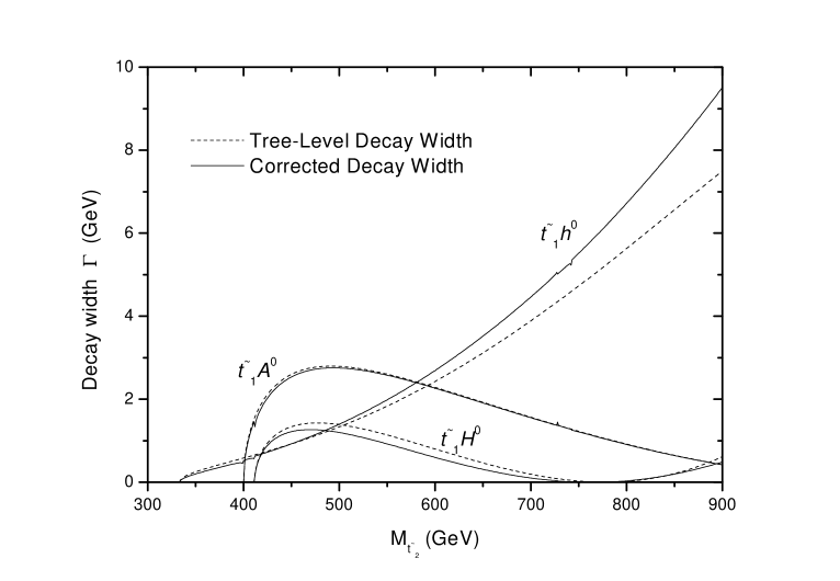
Figure 10: The decay width of $\tilde{t}_{2}\rightarrow\tilde{t}_{1}H^{0}_{i}$ as a function of $m_{\tilde{t_{2}}}$, assuming $\tan\beta=3$,$\cos\theta_{\tilde{t}}=0.26$, $m_{\tilde{t}_{1}}=250$GeV, $\mu=550$GeV, $m_{\tilde{g}}=600$GeV, $A_{t}=A_{b}$, $m_{A^{0}}=150$GeV and $M_{\tilde{D}}=1.12M_{\tilde{Q}}$. The solid lines correspond to the Yukawa-corrected decay widths, The dashed lines correspond to the tree-level decay widths.

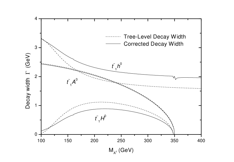
Figure 11: The decay width of $\tilde{t}_{2}\rightarrow\tilde{t}_{1}H^{0}_{i}$ as a function of $m_{A^{0}}$, assuming $\tan\beta=3$,$\cos\theta_{\tilde{t}}=0.26$, $m_{\tilde{t}_{1}}=250$GeV, $\mu=550$GeV, $m_{\tilde{g}}=600$GeV, $A_{t}=A_{b}$ and $M_{\tilde{D}}=1.12M_{\tilde{Q}}$. The solid lines correspond to the Yukawa-corrected decay widths, The dashed lines correspond to the tree-level decay widths.

(ii) For the parameters $m^{2}_{\tilde{Q},\tilde{U},\tilde{D}}$ and $A_{t,b}$ in squark mass matrices, we assumed $M_{\tilde{Q}}=1.5M_{\tilde{U}}=1.5M_{\tilde{D}}$ and $A_{t}=A_{b}$ to simplify the calculations, except for Figs.10-11, where we assumed $M_{\tilde{D}}=1.12M_{\tilde{Q}}$ and $A_{t}=A_{b}$ in order to compare with the SUSY-QCD results in Ref.[8].

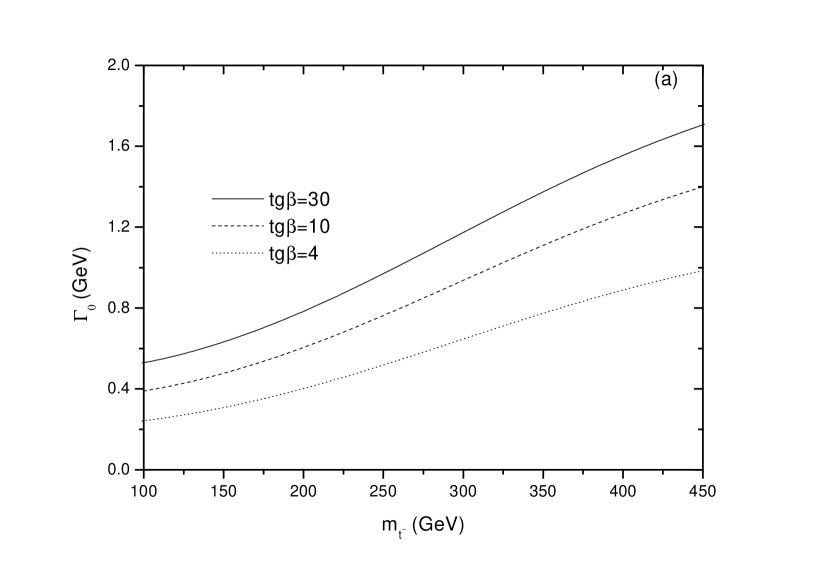
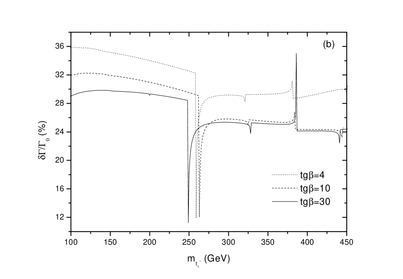
Figure 3: The tree-level decay width $(a)$ of $\tilde{t}_{2}\rightarrow\tilde{t}_{1}h^{0}$ and its Yukawa corrections $(b)$ as functions of $m_{\tilde{t}_{1}}$ for $\tan\beta=4$, $10,$ and $30$, respectively, assuming $m_{A^{0}}=150$GeV, $\mu=M_{2}=200$GeV, $A_{t}=A_{b}=600$GeV and $M_{\tilde{Q}}=1.5M_{\tilde{U}}=1.5M_{\tilde{D}}$.

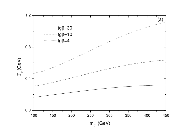
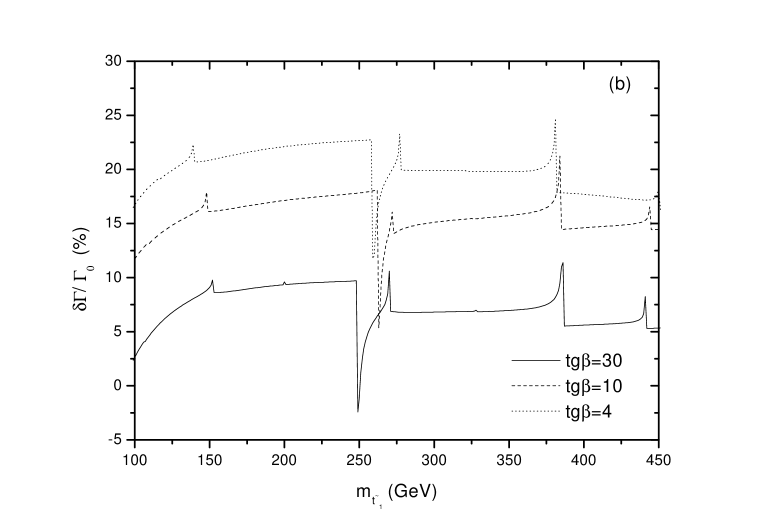
Figure 4: The tree-level decay width $(a)$ of $\tilde{t}_{2}\rightarrow\tilde{t}_{1}H^{0}$ and its Yukawa corrections $(b)$ as functions of $m_{\tilde{t}_{1}}$ for $\tan\beta=4$, 10, and 30, respectively, assuming $m_{A^{0}}=150$GeV, $\mu=M_{2}=200$GeV, $A_{t}=A_{b}=600$GeV and $M_{\tilde{Q}}=1.5M_{\tilde{U}}=1.5M_{\tilde{D}}$.

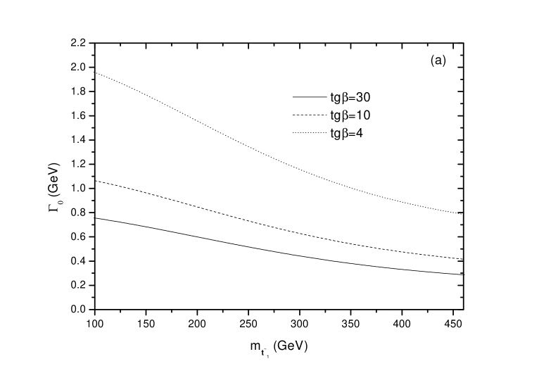
Figure 5: The tree-level decay width $(a)$ of $\tilde{t}_{2}\rightarrow\tilde{t}_{1}A^{0}$ and its Yukawa corrections $(b)$ as functions of $m_{\tilde{t}_{1}}$ for $\tan\beta=4$, $10,$ and $30$, respectively, assuming $m_{A^{0}}=150$GeV, $\mu=M_{2}=200$GeV, $A_{t}=A_{b}=600$GeV and $M_{\tilde{Q}}=1.5M_{\tilde{U}}=1.5M_{\tilde{D}}$.

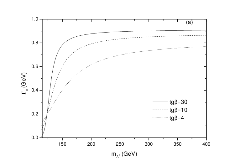
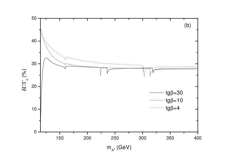
Figure 6: The tree-level decay width $(a)$ of $\tilde{t}_{2}\rightarrow\tilde{t}_{1}h^{0}$ and its Yukawa corrections $(b)$ as functions of $m_{A^{0}}$ for $\tan\beta=4$, $10,$ and $30$, respectively, assuming $m_{\tilde{t}_{1}}=200$GeV, $\mu=M_{2}=200$GeV, $A_{t}=A_{b}=600$GeV and $M_{\tilde{Q}}=1.5M_{\tilde{U}}=1.5M_{\tilde{D}}$.

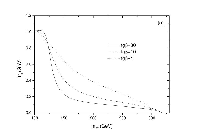
Figure 7: The tree-level decay width $(a)$ of $\tilde{t}_{2}\rightarrow\tilde{t}_{1}H^{0}$ and its Yukawa corrections $(b)$ as functions of $m_{A^{0}}$ for $\tan\beta=4$, $10$, and $30$, respectively, assuming $m_{\tilde{t}_{1}}=200$GeV, $\mu=M_{2}=200$GeV, $A_{t}=A_{b}=600$GeV and $M_{\tilde{Q}}=1.5M_{\tilde{U}}=1.5M_{\tilde{D}}$.

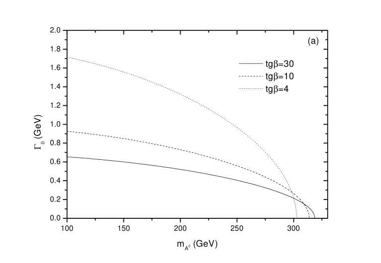
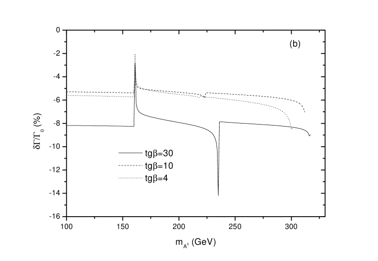
Figure 8: The tree-level decay width $(a)$ of $\tilde{t}_{2}\rightarrow\tilde{t}_{1}A^{0}$ and its Yukawa corrections $(b)$ as functions of $m_{A^{0}}$ for $\tan\beta=4$, $10,$ and $30$, respectively, assuming $m_{\tilde{t}_{1}}=200$GeV, $\mu=M_{2}=200$GeV, $A_{t}=A_{b}=600$GeV, and $M_{\tilde{Q}}=1.5M_{\tilde{U}}=1.5M_{\tilde{D}}$.

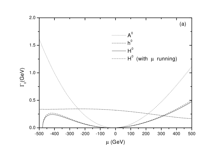
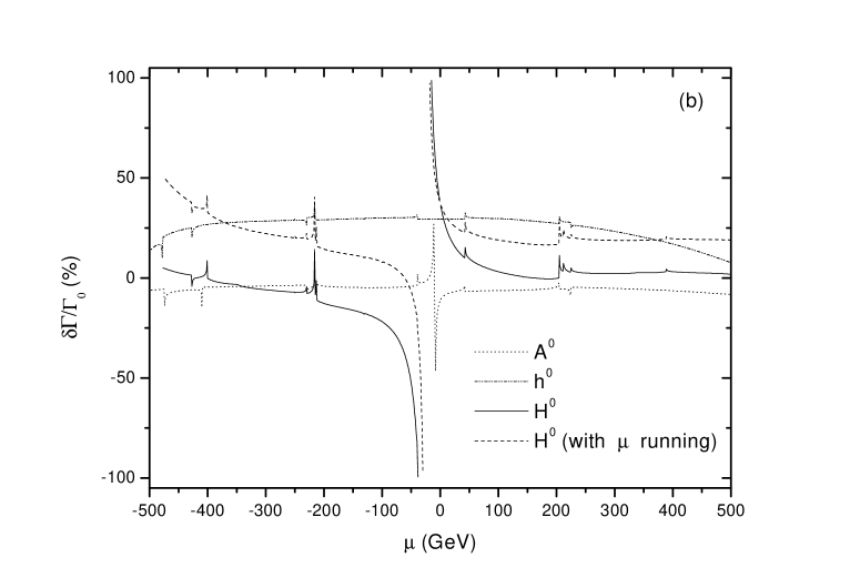
Figure 9: The tree-level decay width $(a)$ of $\tilde{t}_{2}\rightarrow\tilde{t}_{1}H^{0}_{i}$ and its Yukawa corrections $(b)$ as functions of $\mu$, assuming $\tan\beta=30$, $m_{\tilde{t}_{1}}=250$GeV, $M_{2}=100$GeV, $A_{t}=250GeV$,$A_{b}=-250$GeV, $m_{A^{0}}=150$GeV and $M_{\tilde{Q}}=1.5M_{\tilde{U}}=1.5M_{\tilde{D}}$.

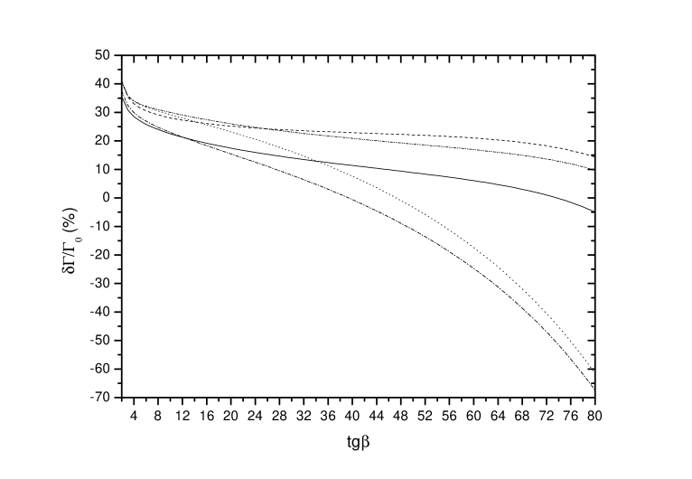
Figure 12: The Yukawa corrections of $\tilde{t}_{2}\rightarrow\tilde{t}_{1}H^{0}$ as a function of $\tan\beta$, assuming $m_{\tilde{t}_{1}}=250$GeV, $M_{2}=200$GeV, $A_{t}=A_{b}=900$GeV, $\mu=200$GeV, $m_{A^{0}}=150$GeV and $M_{\tilde{Q}}=1.5M_{\tilde{U}}=1.5M_{\tilde{D}}$. The dotted line corresponds to the corrections using the on-shell parameters; the dashed line corresponds to the corrections using the running parameters $\hat{m}_{t}(Q)$, $\hat{m}_{b}(Q)$, $\hat{A}_{t}$, and $\hat{\mu}$; the solid line corresponds to the corrections using the same running parameters except the running $\hat{\mu}$; the dashed-dotted line to the improved result only using the running mass $\hat{m}_{t}(Q)$; and the dash-dot-doted line to the improved result only using the running mass $\hat{m}_{b}(Q)$.

Some typical numerical results of the tree-level decay widths and the Yukawa corrections are given in Figs.3-12.

Figs.3 - 5 show the $m_{\tilde{t}_{1}}$ dependence of the results of the three decay channels, respectively. Here we take $m_{A^{0}}=150$GeV, $\mu=M_{2}=200$GeV, and $A_{t}=A_{b}=600$GeV. The leading terms of the tree-level amplitudes $M^{(0)}_{s}$(s=1,2,3) are given by

$$M^{(0)}_{1}=\frac{-ig\hat{m}_{t}}{2m_{W}\sin\beta}(\hat{A}_{t}\cos\alpha+\mu\sin\alpha)\cos 2\theta_{\tilde{t}}\hskip 2.84544pt,$$ (54)

$$M^{(0)}_{2}=\frac{-ig\hat{m}_{t}}{2m_{W}\sin\beta}(\hat{A}_{t}\sin\alpha-\mu\cos\alpha)\cos 2\theta_{\tilde{t}}\hskip 2.84544pt,$$ (55)

$$M^{(0)}_{3}=\frac{-g\hat{m}_{t}}{2m_{W}}(\hat{A}_{t}\cot\beta+\mu)\hskip 2.84544pt.$$ (56)

For $m_{\tilde{t}_{1}}$=100GeV, $\cos\theta_{\tilde{t}}\sim$ (-0.575, -0.574, -0.574) and $\cos\alpha\sim$ (0.754, 0.953, 1.000) for $\tan\beta=$ 4, 10, and 30 , respectively, and for $m_{\tilde{t}_{1}}$=560GeV, $\cos\theta_{\tilde{t}}\sim$ (-0.323, -0.332, -0.334) and $\cos\alpha\sim$ (0.737, 0.897, 0.992) for $\tan\beta\sim$ 4, 10, and 30, respectively. In the case of $i=2$, the two terms in Eq.(55) have opposite signs, and their magnitudes get close with the increasing $\tan\beta$ and thus cancel to large extent for large $\tan\beta$. Therefore, the tree-level decay widths have the feature of $\Gamma_{0}(\tan\beta=4)>\Gamma_{0}(\tan\beta=10)>\Gamma_{0}(\tan\beta=30)$ in most range of the parameter space, as shown in Fig.4(a). In the case of $i=1$, the two terms in Eq.(54) have the same signs, there are not cancelling effects between them, so $\Gamma_{0}$ is larger than the one of the case of $i=2$ for the same values of $\tan\beta$. In the case of $i=3$, the amplitude contains a term propotional to $\cot\beta$, so $\Gamma_{0}(\tan\beta=4)>\Gamma_{0}(\tan\beta=10)>\Gamma_{0}(\tan\beta=30)$. From Figs.3-5(b), one can see that the relative corrections are sensitive to the value of $\tan\beta$. For $\tan\beta=$ 4 and 30, the magnitudes of the corrections can exceed $30\%$ and $20\%$ , respectively, for the decay into $h^{0}$ . For $\tan\beta=$ 10, the corrections to the widths of the three decay channels are smaller than ones either in the case of $\tan\beta=$ 4 or in the case of $\tan\beta=$ 30 . In general, for low $\tan\beta$ the top quark contribution is enhanced while for high $\tan\beta$ the bottom quark contribution become large, and for medium $\tan\beta$, there are not any the enhanced effects from the Yukawa couplings. So the corrections for $\tan\beta=$ 4 or 30 are generally larger than those for $\tan\beta$ =10, as shown in Figs.3-5(b). There are some dips and peaks in Figs.3-5(b), which arise from the singularities at the threshold points $m_{\tilde{t}_{1}}=m_{\tilde{\chi}^{0}_{i}}+m_{t}$ and $m_{\tilde{t}_{2}}=m_{\tilde{b}_{2}}+m_{G^{+}}(=m_{W})$, respectively.

Figs.6-8 give the tree-level decay widths and the Yukawa corrections as the functions of $m_{A^{0}}$ for the three decays. We assumed $m_{\tilde{t}_{1}}=200$GeV, $\mu=M_{2}=200$GeV and $A_{t}=A_{b}=1$TeV. The features of the tree level decay widths in Figs.6-8(a) are similar to Figs.3-5(a) , respectively. From Figs.6-8(b) we can see that the relative corrections decrease or increase the decay widths depending on $\tan\beta$. In most range of the mass of $A^{0}$, the relative corrections vary from 27% to 33% for the decay into $h^{0}$, -6% to 20% for the decay into $H^{0}$, and -9% to -5% for the decay into $A^{0}$. There are many dips and peaks on the curves in Figs.6-8(b), which come from the singularities at the threshold points. For example, at $m_{A^{0}}=235$GeV in Fig.8(b) , we have the threshold point $m_{\tilde{b}_{1}}=m_{\tilde{\chi}^{0}_{4}}+m_{b}$ for $\tan\beta=30$.

In Fig.9 we present the tree-level decay widths and the Yukawa corrections as the functions of $\mu$ in the case of $\tilde{t}_{2}\rightarrow\tilde{t}_{1}+H^{0}_{i}$ , assuming $\tan\beta=30$, $m_{\tilde{t}_{1}}=250$GeV, $M_{2}=100$GeV, $A_{t}=250$GeV, $A_{b}=-250$GeV and $m_{A^{0}}=150$GeV. In most of the parameter $\mu$ range , the relative corrections are about from 12% to 32% for the decay into $h^{0}$, and only a few percent for the decay into $A^{0}$ except near the zero point of $\Gamma_{0}$ . For the decay into $H^{0}$, when $\mu$ takes certain values (near about -26 GeV), $\Gamma_{0}$ gets very small ($<10^{-4}$GeV), and the relative corrections near these values do not have a physical meaning. So we cut off the corrections, since perturbation theory breaks down here. In order to improve the results, we use the running higgsino mass parameter $\hat{\mu}(Q)=\mu+\delta\hat{\mu}(Q)$ in the tree-level coupling, and find that the convergence of the perturbation expansion becomes better as shown by the dashed line in Fig.9(b), where the region of the parameter $\mu$ of breaking down the perturbation theory gets smaller (Note that, in fact, the parameter range $|\mu|<180$ GeV has been excluded by phenomenology at LEP and Tevatron [16, 31] ). There are many dips and peaks on the curves in Fig.9(b), which come from the singularities at the threshold points. For example, at $\mu=-216$ GeV on the solid curve in Fig.9(b) , we have the threshold point $m_{\tilde{t}_{2}}=m_{\chi^{0}_{4}}+m_{t}$ for the decay into $H^{0}$.

In Figs.10-11 we compare the results with the ones presented in an earlier literature [9] where the ${\cal O}(\alpha_{s})$ SUSY-QCD corrections to the same three decay processes have been calculated. We present the tree-level decay widths and the Yukawa corrected decay widths as the functions of $m_{\tilde{t}_{2}}$ and $m_{A^{0}}$ in Figs.10 and 11, respectively . For comparation, we take the same input parameters as in the Ref.[9] : $\tan\beta=3$, $\cos\theta_{\tilde{t}}=0.26$, $m_{\tilde{t}_{1}}=250$GeV, $m_{\tilde{g}}=600$GeV, $\mu=550$GeV in Figs.10-11, and $m_{A^{0}}=150$GeV in Fig.10, $m_{\tilde{t}_{2}}=600$GeV in Fig.11. In both Figs, we assumed $M_{\tilde{D}}=1.12M_{\tilde{Q}}$. Our numerical results of the tree level decay widths agree with their results except a little difference, which is due to the running effects were used in our calculation but not in Ref.[9]. The relative corrections in Fig.10 vary from -22% to 26% for the decay into $h^{0}$, -60% to -4% for the decay into $H^{0}$, and -5% to 0% for the decay into $A^{0}$. The relative corrections in Fig.11 vary from -1% to 23% for the decay into $h^{0}$, -24% to 60% for the decay into $H^{0}$, -4% to -1% for the decay into $A^{0}$. After comparing with Figs.3 and 5 in Ref.[9], we can see that the Yukawa corrections are comparable to the ${\cal O}(\alpha_{s})$ SUSY-QCD corrections for the decays into $h^{0}$ and $H^{0}$, but smaller than the ${\cal O}(\alpha_{s})$ SUSY-QCD corrections for the decays into $A^{0}$. There are two dips at $m_{A^{0}}=348$GeV and 352GeV on the solid curve of the decay into $h_{0}$ in Fig.11, which come from the singularities at the threshold points $m_{\tilde{t}_{2}}=m_{\tilde{t}_{1}}+m_{H^{0}}.$

Finally, in Fig.12 we show the numerical improvement of the Yukawa corrections as a function of $\tan\beta$ in five ways of perturbative expansion: (i) the strict on-shell scheme (the dotted line), where the top quark pole mass 175.6GeV, the bottom quark pole mass 4.25GeV, the on-shell trilinear coupling $A_{t}$ and the higssino mass parameter $\mu$ were used, (ii) the improved scheme (the solid line), in which the QCD, SUSY-QCD, and SUSY-Electroweak running quark masses $\hat{m}_{q}(Q)$ and the running trilinear coupling $\hat{A}_{t}(Q)$ were used, (iii) the complete improved scheme (the dashed line), in which the SUSY-Electroweak running parameter $\mu$ was also used as well as the same running parameters as in (ii),    (iv) the $\hat{m}_{t}(Q)$ running scheme (the dash-dotted line), in which only the running top quark mass was used, and (v) the $\hat{m}_{b}(Q)$ running scheme (the dash-dot-dotted line), in which only the running bottom quark mass was used. Here we assumed $m_{\tilde{t}_{1}}=250$GeV, $M_{2}=200$GeV, $A_{t}=A_{b}=900$GeV, $\mu=200$GeV, $m_{A^{0}}=150$GeV and $M_{\tilde{Q}}=1.5M_{\tilde{U}}=1.5M_{\tilde{D}}$. One can see that, the effect of the running of the top quark mass on the corrections can not be neglected for low $\tan\beta(<10)$, while the effect of the running of the bottom quark mass is quite significant for large $\tan\beta(>40)$ . The whole running effects with or without the running of the parameter $\mu$ both make the convergence of the perturbation expansion much better. The relative corrections approach smoothly -5.0% and 14.3% with the increasing $\tan\beta$ for the improved scheme and complete improved scheme, as shown by the solid line and the dashed line in Fig.12, respectively.

In conclusion, we have calculated the Yukawa corrections to the widths of the heavier top squark decays into lighter top squarks and neutral Higgs bosons in the MSSM. These corrections depend on the masses of the neutral Higgs bosons and the lighter or heavier top squark, and the parameter $\mu$. For favorable parameter values, the corrections decrease or increase the tree-level decay widths significantly. Especially, for high values of $\tan\beta$(=30) or low values of $\tan\beta$(=4), the magnitudes of the corrections exceed at least $20\%$ for the decay into $h^{0}$ and $H^{0}$, which are comparable to the ${\cal O}(\alpha_{s})$ SUSY-QCD corrections. But for the decay into $A^{0}$, the corrections are smaller and the magnitudes of them are less than $10\%$ in most of the parameter space. The numerical calculations also show that using the running quark masses and the running trilinear coupling $A_{t}$ , which include the QCD, SUSY-QCD, and SUSY-Electroweak effects and resume all high order ($\tan\beta$)-enhanced effects, can vastly improve the convergence of the perturbation expansion. We also discuss the effects of the running of the higgsino mass parameter $\mu$ on the corrections, and find that they are significant, too, especially for large $\tan\beta$.

Appendix A

The following couplings are given in order $O(h_{t},h_{b})$.

1. squark – squark – Higgs boson

(a) squark – squark – $h^{0}$

$$\hat{G}^{\tilde{q}}_{1}=\left(\begin{array}[]{cc}-\sqrt{2}m_{q}h_{q}\left\{\begin{array}[]{c}c_{\alpha}\\ -s_{\alpha}\end{array}\right\}&-\frac{1}{\sqrt{2}}h_{q}(A_{q}\left\{\begin{array}[]{c}c_{\alpha}\\ -s_{\alpha}\end{array}\right\}+\mu\left\{\begin{array}[]{c}s_{\alpha}\\ -c_{\alpha}\end{array}\right\})\\ -\frac{1}{\sqrt{2}}h_{q}(A_{q}\left\{\begin{array}[]{c}c_{\alpha}\\ -s_{\alpha}\end{array}\right\}+\mu\left\{\begin{array}[]{c}s_{\alpha}\\ -c_{\alpha}\end{array}\right\})&-\sqrt{2}m_{q}h_{q}\left\{\begin{array}[]{c}c_{\alpha}\\ -s_{\alpha}\end{array}\right\}\end{array}\right)$$ (71)

for $\left\{\begin{array}[]{c}{\rm up}\\ {\rm down}\end{array}\right\}$ type squarks, respectively. We use the abbreviations $s_{\alpha}=\sin\alpha$, $c_{\alpha}=\cos\alpha$. $\alpha$ is the mixing angle in the CP even neutral Higgs boson sector.

(b) squark – squark – $H^{0}$

$$\hat{G}^{\tilde{q}}_{2}=\left(\begin{array}[]{cc}-\sqrt{2}m_{q}h_{q}\left\{\begin{array}[]{c}s_{\alpha}\\ c_{\alpha}\end{array}\right\}&-\frac{1}{\sqrt{2}}h_{q}(A_{q}\left\{\begin{array}[]{c}s_{\alpha}\\ c_{\alpha}\end{array}\right\}-\mu\left\{\begin{array}[]{c}c_{\alpha}\\ s_{\alpha}\end{array}\right\})\\ -\frac{1}{\sqrt{2}}h_{q}(A_{q}\left\{\begin{array}[]{c}s_{\alpha}\\ c_{\alpha}\end{array}\right\}-\mu\left\{\begin{array}[]{c}c_{\alpha}\\ s_{\alpha}\end{array}\right\})&-\sqrt{2}m_{q}h_{q}\left\{\begin{array}[]{c}s_{\alpha}\\ c_{\alpha}\end{array}\right\}\end{array}\right)$$ (86)

(c) squark – squark – $A^{0}$

$$\hat{G}^{\tilde{q}}_{3}=i\frac{gm_{q}}{2m_{W}}\left(\begin{array}[]{cc}0&-A_{q}\left\{\begin{array}[]{c}\cot\beta\\ \tan\beta\end{array}\right\}-\mu\\ A_{q}\left\{\begin{array}[]{c}\cot\beta\\ \tan\beta\end{array}\right\}+\mu&0\end{array}\right)$$ (93)

(d) squark – squark – $G^{0}$

$$\hat{G}^{\tilde{q}}_{4}=-i\frac{gm_{q}}{2m_{W}}\left(\begin{array}[]{cc}0&-A_{q}+\mu\left\{\begin{array}[]{c}\cot\beta\\ \tan\beta\end{array}\right\}\\ A_{q}-\mu\left\{\begin{array}[]{c}\cot\beta\\ \tan\beta\end{array}\right\}&0\end{array}\right)$$ (100)

(e) squark – squark – $H^{\pm}$

$$\hat{G}^{\tilde{b}}_{5}=(\hat{G}^{\tilde{t}}_{5})^{T}=\frac{g}{\sqrt{2}m_{W}}\left(\begin{array}[]{cc}m_{b}^{2}\tan\beta+m_{t}^{2}\cot\beta&m_{t}(A_{t}\cot\beta+\mu)\\ m_{b}(A_{b}\tan\beta+\mu)&2m_{t}m_{b}/\sin 2\beta\end{array}\right)$$ (103)

(f) squark – squark – $G^{\pm}$

$$\hat{G}^{\tilde{b}}_{6}=(\hat{G}^{\tilde{t}}_{6})^{T}=\frac{-g}{\sqrt{2}m_{W}}\left(\begin{array}[]{cc}m_{t}^{2}-m_{b}^{2}&m_{t}(A_{t}-\mu\cot\beta)\\ m_{b}(\mu\tan\beta-A_{b})&0\end{array}\right)$$ (106)

2. quark – quark – Higgs boson

$$a_{k}^{q}=(\frac{1}{\sqrt{2}}h_{q}\left\{\begin{array}[]{c}-c_{\alpha}\\ s_{\alpha}\end{array}\right\},-\frac{1}{\sqrt{2}}h_{q}\left\{\begin{array}[]{c}s_{\alpha}\\ c_{\alpha}\end{array}\right\},-\frac{i}{\sqrt{2}}h_{q}\left\{\begin{array}[]{c}\cos\beta\\ \sin\beta\end{array}\right\},\frac{-ig}{2m_{W}}\left\{\begin{array}[]{c}-m_{t}\\ m_{b}\end{array}\right\},$$ (115)

$$\hskip 85.35826pt\left\{\begin{array}[]{c}h_{b}\sin\beta\\ h_{t}\cos\beta\end{array}\right\},\frac{g}{\sqrt{2}m_{W}}\left\{\begin{array}[]{c}-m_{b}\\ m_{t}\end{array}\right\})$$ (120)

$$b_{k}^{q}=(\frac{1}{\sqrt{2}}h_{q}\left\{\begin{array}[]{c}-c_{\alpha}\\ s_{\alpha}\end{array}\right\},-\frac{1}{\sqrt{2}}h_{q}\left\{\begin{array}[]{c}s_{\alpha}\\ c_{\alpha}\end{array}\right\},-\frac{i}{\sqrt{2}}h_{q}\left\{\begin{array}[]{c}\cos\beta\\ \sin\beta\end{array}\right\},\frac{-ig}{2m_{W}}\left\{\begin{array}[]{c}m_{t}\\ -m_{b}\end{array}\right\},$$ (129)

$$\hskip 85.35826pth_{q}\left\{\begin{array}[]{c}\cos\beta\\ \sin\beta\end{array}\right\},\frac{g}{\sqrt{2}m_{W}}\left\{\begin{array}[]{c}m_{t}\\ -m_{b}\end{array}\right\})$$ (134)

3. quark – squark – neutralino

$$a_{ik}^{\tilde{q}}=-R_{i2}^{\tilde{q}}Y_{q}\left\{\begin{array}[]{c}N_{k4}\\ N_{k3}\end{array}\right\},\hskip 42.67912ptb_{ik}^{\tilde{q}}=-R_{i1}^{\tilde{q}}Y_{q}\left\{\begin{array}[]{c}N_{k4}^{\ast}\\ N_{k3}^{\ast}\end{array}\right\}$$ (139)

Here $N$ is the $4\times 4$ unitary matrix diagonalizing the neutral gaugino-higgsino mass matrix [2, 30].

4. quark – squark – chargino

$$l_{ik}^{\tilde{q}}=R_{i2}^{\tilde{q}}Y_{q}\left\{\begin{array}[]{c}V_{k2}\\ U_{k2}\end{array}\right\},\hskip 42.67912ptk_{ik}^{\tilde{q}}=R_{i1}^{\tilde{q}}\left\{\begin{array}[]{c}Y_{b}U_{k2}\\ Y_{t}V_{k2}\end{array}\right\}.$$ (144)

Here $U$ and $V$ are the $2\times 2$ unitary matrices diagonalizing the charged gaugino–higgsino mass matrix [2, 30].

5. squark – squark – Higgs boson – Higgs boson

(a) squark – squark – $H^{-}$ – $H_{k}$ (k=1,2)

$$\hat{G}_{5k}^{\tilde{b}}=(\hat{G}_{5k}^{\tilde{t}})^{T}=\frac{g^{2}}{2\sqrt{2}m_{W}^{2}}\left(\begin{array}[]{cc}m_{t}^{2}S_{k}+m_{b}^{2}T_{k}&0\\ 0&\frac{2m_{t}m_{b}}{\sin 2\beta}V_{k}\end{array}\right)$$ (147)

with

$$S_{k}=(\cos\alpha\cos\beta/\sin^{2}\beta,\ \ \ \sin\alpha\cos\beta/\sin^{2}\beta)$$ (148)

$$T_{k}=(-\sin\alpha\sin\beta/\cos^{2}\beta,\ \ \ \cos\alpha\sin\beta/\cos^{2}\beta)$$ (149)

$$V_{k}=(\sin(\beta-\alpha),\ \ \ \cos(\beta-\alpha))$$ (150)

(b) squark – squark – $H^{-}$ – $H^{+}$

$$\hat{G}_{55}^{\tilde{q}}=\left(\begin{array}[]{cc}-\left\{\begin{array}[]{c}h_{b}^{2}\sin^{2}\beta\\ h_{t}^{2}\cos^{2}\beta\end{array}\right\}&0\\ 0&-h_{q}^{2}\left\{\begin{array}[]{c}\cos^{2}\beta\\ \sin^{2}\beta\end{array}\right\}\end{array}\right)$$ (157)

(c) squark – squark – $H^{-}$ – $G^{+}$

$$\hat{G}_{56}^{\tilde{q}}=-\frac{g^{2}}{2m_{W}^{2}}\left(\begin{array}[]{cc}\left\{\begin{array}[]{c}-m_{b}^{2}\tan\beta\\ m_{t}^{2}\cot\beta\end{array}\right\}&0\\ 0&m_{q}^{2}\left\{\begin{array}[]{c}\cot\beta\\ -\tan\beta\end{array}\right\}\end{array}\right)$$ (164)

(d) squark – squark – $G^{-}$ – $H_{k}$ (k=1,2,3)

$$\hat{G}_{6k}^{\tilde{b}}=(\hat{G}_{6k}^{\tilde{t}})^{T}=\frac{g^{2}}{2\sqrt{2}m_{W}^{2}}\left(\begin{array}[]{cc}m_{t}^{2}\hskip 5.69046ptSG_{k}+m_{b}^{2}\hskip 5.69046ptTG_{k}&0\\ 0&2m_{t}m_{b}/\sin 2\beta\hskip 5.69046ptVG_{k}\end{array}\right)$$ (167)

with

$$SG_{k}=(\cos\alpha/\sin\beta,\ \ \ \sin\alpha/\sin\beta\ \ \ i\cot\beta)$$ (168)

$$TG_{k}=(\sin\alpha/\cos\beta,\ \ \ -\cos\alpha/\cos\beta\ \ \ i\tan\beta)$$ (169)

$$VG_{k}=(-\cos(\beta-\alpha),\ \ \ \sin(\beta-\alpha)\ \ \ -i)$$ (170)

(e) squark – squark – $H_{k}$ – $H_{k}$ (k=1,2,3)

$$\hat{G}_{kk}^{\tilde{t}}=\left(\begin{array}[]{cc}\frac{-g^{2}}{2m_{W}^{2}}m_{t}^{2}\hskip 2.84544pt{D1}_{k}&0\\ 0&\frac{-g^{2}}{2m_{W}^{2}}m_{t}^{2}\hskip 2.84544pt{D1}_{k}\end{array}\right)$$ (173)

with

$${D1}_{k}=(\sin^{2}\alpha/\sin^{2}\beta,\ \ \ \cos^{2}\alpha/\sin^{2}\beta,\ \ \ \cot^{2}\beta)$$ (174)

$$\hat{G}_{kk}^{\tilde{b}}=\left(\begin{array}[]{cc}\frac{-g^{2}}{2m_{W}^{2}}m_{b}^{2}\hskip 2.84544pt{D2}_{k}&0\\ 0&\frac{-g^{2}}{2m_{W}^{2}}m_{b}^{2}\hskip 2.84544pt{D2}_{k}\end{array}\right)$$ (177)

with

$${D2}_{k}=(\cos^{2}\alpha/\sin^{2}\beta,\ \ \ \sin^{2}\alpha/\sin^{2}\beta,\ \ \ \tan^{2}\beta)$$ (178)

(f) squark – squark – $H^{0}$ – $h^{0}$

$$\hat{G}_{12}^{\tilde{b}}=\left(\begin{array}[]{cc}\frac{-g^{2}m_{b}^{2}\sin 2\alpha}{4m_{W}^{2}}\hskip 2.84544ptD2&0\\ 0&\frac{-g^{2}m_{b}^{2}\sin 2\alpha}{4m_{W}^{2}}\hskip 2.84544ptD2\end{array}\right)$$ (181)

with $D2=-1/\cos^{2}\beta$

$$\hat{G}_{12}^{\tilde{t}}=\left(\begin{array}[]{cc}\frac{-g^{2}m_{t}^{2}\sin 2\alpha}{4m_{W}^{2}}\hskip 2.84544ptD1&0\\ 0&\frac{-g^{2}m_{t}^{2}\sin 2\alpha}{4m_{W}^{2}}\hskip 2.84544ptD1\end{array}\right)$$ (184)

with $D1=-1/\sin^{2}\beta$

(g) squark – squark – $A^{0}$ – $G^{0}$

$$\hat{G}_{35}^{\tilde{b}}=\left(\begin{array}[]{cc}\frac{-g^{2}m_{b}^{2}\sin 2\beta}{4m_{W}^{2}}\hskip 2.84544ptD2&0\\ 0&\frac{-g^{2}m_{b}^{2}\sin 2\beta}{4m_{W}^{2}}\hskip 2.84544ptD2\end{array}\right)$$ (187)

$$\hat{G}_{35}^{\tilde{t}}=\left(\begin{array}[]{cc}\frac{-g^{2}m_{b}^{2}\sin 2\beta}{4m_{W}^{2}}\hskip 2.84544ptD1&0\\ 0&\frac{-g^{2}m_{b}^{2}\sin 2\beta}{4m_{W}^{2}}\hskip 2.84544ptD1\end{array}\right)$$ (190)

Finally, we define$\hat{G}_{ji}^{\tilde{q}}=\hat{G}_{ij}^{\tilde{q}},$ and also $\hat{G}_{3(4)k}^{\tilde{q}}=0$, when k=1,2,5, i.e. there are no $A^{0}(G^{0})h^{0}\tilde{q}\tilde{q}$,$A^{0}(G^{0})H^{0}\tilde{q}\tilde{q}$, or $A^{0}(G^{0})H^{+}\tilde{q}\tilde{q}$ couplings.

Appendix B

We define $q=t$ and $b$, $q^{\prime}$ the $SU(2)_{L}$ partner of $q$, and $q^{\prime\prime}=q$ for $k=1...4$ and $q^{\prime\prime}=q^{\prime}$ for $k=5,6$. Then we have

Here $A_{0}$ and $B_{1}$ are one- and two-point Feynman integrals[20], respectively, and $G_{1}=\partial B_{1}/\partial p^{2}$,$G_{0}=-\partial B_{0}/\partial p^{2}$.

Figure 1: Feynman diagrams contributing to supersymmetric electroweak corrections to $\tilde{t}_{2}\rightarrow\tilde{t}_{1}H_{i}$:   $H_{i}$, i=1,2,3 correspond to $h^{0},H^{0},A^{0}$. $(a)$ is tree level diagram; $(b)-(f)$ are one-loop vertex corrections. In diagram $(b)$ $q=t$ for $k=1...4$ and $q=b$ for $k=5,6$. In diagram $(d)$ and $(e)$ $q=t$ for $k=1,2$ and $q=b$ for $k=5,6$. In diagram $(f)$, $q=b,t$

Figure 2: Feynman diagrams contributing to renormalization constants. In diagram $(i)$ $q=t(b)$ for $k=1...4$ and $q=b(t)$ for $k=5,6$. In diagram $(f)$ $(g)$ $(h)$ $i=j=1,2,3$ or $i=1,j=2$

References

• [1] H.P. Nilles, Phys. Rep. 110, 1 (1984); A.B. Lahanas, D.V. Nanopoulos, ibid. 145, 1 (1987); Supersymmetry, Vols. 1 and 2, edited by S.Ferrara (North Holland/World Scientific, Singapore, 1987).
• [2] H.E. Haber and G.L. Kane, Phys. Rep. 117, 75 (1985).
• [3] Atlas Collaboration, Atlas Technical Design Report No. CERN/LHCC/99-14/15; CMS Collaboration, CMS Technical Proposal No. CERN/LHCC/94-38; F. Gianotti, in proceedings of the IVth International Symposium on Radiative Corrections (RADCOR 98), edited by J. Sol$\grave{\rm a}$ (World Scientific,Singapore,1999), P.270 .
• [4] D.J. Miller, in proceedings of the IVth International Symposium on Radiative Corrections (RADCOR 98) (Ref.[4] ), p. 289.
• [5] H. Baer, V. Barger, D. Karatas and X. Tata, Phys. Rev. D36, 96 (1987); K. Hikasa and M. Kobayashi, ibid. D36, 724 (1987); R.M. Barnett, J.F. Gunion and H.E. Haber, ibid. D37, 1892 (1988); H. Baer, X. Tata and J. Woodside, ibid. D42, 1568 (1990); K. Hikasa and M. Drees, Phys. Lett. B252, 127 (1990); A. Bartl, W. Majerotto, B. M$\ddot{\rm o}$sslacher and N. Oshimo, Z. Phys. C52, 477 (1991); A. Bartl, W. Majerotto and W. Porod, ibid. C64, 499 (1994); C68, 518(E) (1995).
• [6] A. Bartl, H. Eberl, K. Hidaka, S. Kraml, T. Kon, W. Majerotto, W. Porod and Y. Yamada, Phys. Lett. B435, 118 (1998).
• [7] K. Hidaka and A. Bartl, Phys. Lett. B501, 78 (2001).
• [8] S. Kraml, H. Eberl, A. Bartl, W. Majerotto and W. Porod, Phys. Lett. B386, 175 (1996); A. Djouadi, W. Hollik and C. J$\ddot{\rm u}$nger, Phys. Rev. D55, 6975 (1997).
• [9] A. Bartl, H. Eberl, K. Hidaka, S. Kraml, W. Majerotto, W. Porod and Y. Yamada, Phys. Lett. B419, 243 (1998), hep-ph/9806299.
• [10] J. Guasch, W. Hollik and J. Sol$\grave{\rm a}$, Phys. Lett. B437, 88 (1998).
• [11] J. Guasch, W. Hollik and J. Sol$\grave{\rm a}$, Phys. Lett. B510, 211 (2001), hep-ph/0101086.
• [12] Hou Hong-Sheng, Ma Wen-Gan , Wan Lang-Hui, Zhang Ren-You , Phys. Rev. D65 (2001).
• [13] Li Lin Yang, Chong Sheng Li and Qiang Li, Preprint,PKU-TH-0206022, to be published.
• [14] A.Bartl, H.Eberl, K.Hidaka, S.Kraml, W.Majerotto, W.Porod and Y.Yamada , Phys. Lett. B419, 243 (1998); Phys. Rev. D59, 115007, (1999).
• [15] Li Gang Jin and Chong Sheng Li , Phys. Rev. D65, 0350 (2001), hep-eh/0106253.
• [16] H.Eberl,K.Hidaka et al., Phys. Rev. D62, 055006 (2000).
• [17] S. Sirlin, Phys. Rev. D22, 971 (1980); W.J. Marciano and A. Sirlin, ibid. D22, 2695 (1980); D31, 213(E) (1985); A. Sirlin and W.J. Marciano, Nucl. Phys. B189, 442 (1981); K.I. Aoki et al., Prog. Theor. Phys. Suppl. 73, 1 (1982).
• [18] R. Santos and A. Barroso, Phys. Rev. D56, 5366 (1997).
• [19] A. Mendez and A. Pomarol, Phys. Lett. B279, 98 (1992).
• [20] G ’t Hooft and M. Veltman, Nucl. Phys. B44, 189 (1972); G. Passarino and M. Veltman, Nucl. Phys. B160, 151 (1979); A. Axelrod, ibid. B209, 349 (1982); M. Clements et al., Phys. Rev. D27, 570 (1983).
• [21] A. Bartl, H. Eberl, K. Hidaka, T. Kon, W. Majerotto and Y. Yamada, Phys. Lett. B402, 303 (1997).
• [22] D. Pierce, A. Papadopoulos, Phys. Rev. D50, 565 (1994).
• [23] H. Eberl, M. Kincel, W. Majerotto and Y. Yamada, Phys. Rev. D64, 115013 (2001), hep-ph/0104109.
• [24] Particle Data Group, C.Caso et al., Eur. Phys. J. C3, 1 (1998).
• [25] M. Carena, D. Garcia , U. Nierste, and C. E. M. Wagner, Nucl. Phys. B577, 88 (2000).
• [26] Damien M.Pierce, Jonathan A.Bagger, Ren Jie Zhang, Nucl. Phys. B491, 3 (1997).
• [27] M. Beneke and A. Signer, Phys. Lett. B471, 233 (1999); A.H. Hoang, Phys. Rev. D61, 034005 (2000).
• [28] S.G. Gorishny, A.L. Kataev, S.A. Larin, and L.R. Surguladze, Mod. Phys. Lett. A5, 2703 (1990); Phys. Rev. D43, 1633 (1991); A. Djouadi, M. Spira, and P.M. Zerwas, Z. Phys. C70, 427 (1996); A. Djouadi, J. Kalinowski, and M. Spira, Comput. Phys. Commun. 108, 56 (1998); M. Spira, Fortschr. Phys. 46, 203 (1998).
• [29] M. Carena, M. Quir$\acute{\rm o}$s, C.E.M. Wagner, Nucl. Phys. B461, 407 (1996).
• [30] P. Nath, R. Arnowitt and A. Chamseddine, Applied $N=1$ Supergravity, ICTP series in Theoretical Physics (World Scientific, Singapore, 1984); J.F. Gunion and H.E. Haber, Nucl. Phys. B272, 1 (1986); L.E. Ib$\acute{\rm a}$ $\tilde{\rm n}$ez and G.G. Ross, hep-ph/9204201, in Perspectives on Higgs Physics, edited by G.L. Kane (World Scientific, Singapore, 1993), hep-ph/9204201
• [31] A.Savoy-Navarro, talk at the International Europhysics Conference on High Energy Physics (HEP99),15. -21. July 1999, Tampere, Finland. For transparencies see http://neutrino.pc.helsinki.fi/hep99/Transparencies/session-07/Savoy-Navarro.pdf.
\DashLine(20,60)(55,60)3 \DashLine(55,60)(85,90)3 \DashLine(55,60)(85,30)3 \Vertex(55,60)1 \Text(15,66)[]$\tilde{t}_{2}$\Text(93,91)[]$\tilde{t}_{1}$\Text(93,29)[]$H_{i}$\Text(55,10)[]$(a)$
\DashLine(15,60)(45,60)3 \DashLine(45,60)(70,77.5)3 \DashLine(70,77.5)(70,42.5)3 \DashLine(70,42.5)(45,60)3 \DashLine(70,77.5)(95,95)3 \DashLine(70,42.5)(95,25)3 \Vertex(45,60)1 \Vertex(70,77.5)1 \Vertex(70,42.5)1 \Text(9,66)[]$\tilde{t}_{2}$\Text(55,80)[]$H_{k}$\Text(55,42)[]$\tilde{q}_{j}$\Text(78,60)[]$\tilde{q}_{l}$\Text(103,96)[]$\tilde{t}_{1}$\Text(103,24)[]$H_{i}$\Text(55,10)[]$(b)$
\DashLine(15,60)(45,60)3 \Line(45,60)(70,77.5) \ArrowLine(70,42.5)(70,77.5) \ArrowLine(45,60)(70,42.5) \DashLine(70,77.5)(95,95)3 \DashLine(70,42.5)(95,25)3 \Vertex(45,60)1 \Vertex(70,77.5)1 \Vertex(70,42.5)1 \Text(9,66)[]$\tilde{t}_{2}$\Text(55,80)[]$\tilde{\chi}_{k}^{0}(\tilde{\chi}^{+}_{k})$\Text(55,45)[]$t(b)$\Text(78,60)[]$t(b)$\Text(103,96)[]$\tilde{t}_{1}$\Text(103,24)[]$H_{i}$\Text(55,10)[]$(c)$
\DashLine(20,60)(55,60)3 \DashCArc(63.5,68.5)(12,0,360)3 \DashLine(72,77)(85,90)3 \DashLine(55,60)(85,30)3 \Vertex(55,60)1 \Vertex(72,77)1 \Text(15,66)[]$\tilde{t}_{2}$\Text(93,91)[]$\tilde{t}_{1}$\Text(93,29)[]$H_{i}$\Text(43,80)[]$H_{k}$\Text(83,63)[]$\tilde{q}_{j}$\Text(55,10)[]$(d)$
\DashLine(12,60)(31,60)3 \DashCArc(43,60)(12,0,360)3 \DashLine(55,60)(85,90)3 \DashLine(55,60)(85,30)3 \Vertex(55,60)1 \Vertex(31,60)1 \Text(7,66)[]$\tilde{t}_{2}$\Text(93,91)[]$\tilde{t}_{1}$\Text(93,29)[]$H_{i}$\Text(43,80)[]$H_{k}$\Text(43,40)[]$\tilde{q}_{j}$\Text(55,10)[]$(e)$
\DashLine(20,60)(55,60)3 \DashLine(55,60)(85,90)3 \DashCArc(63.5,51.5)(12,0,360)3 \DashLine(72,43)(85,30)3 \Vertex(55,60)1 \Vertex(72,43)1 \Text(15,66)[]$\tilde{t}_{2}$\Text(93,91)[]$\tilde{t}_{1}$\Text(93,29)[]$H_{i}$\Text(45,42)[]$\tilde{q}_{l}$\Text(83,63)[]$\tilde{q}_{j}$\Text(55,10)[]$(f)$