Self-tuning solutions of the cosmological constant

Abstract

The self-tuning solutions of the cosmological constant is reviewed, with the emphasis on the recent attempts in extra dimensional gravity with a brane boundary.

Since 1975, the hierarchy problems become the most challenging problems in particle physics:

(i) the gauge hierarchy problemgauge ,

(ii) the cosmological constant problemccp ,

(iii) the strong CP problemstrongcp , and

(iv) the $\mu$ problemmu , etc.

The most severe one among these is the cosmological constant problem in that the hierarchy is the largest and there seems to be no accepted solution in this problem, while the other hierarchy problems leads to some plausible solutions such as supersymmetry, axion, and the introduction of the hidden sector. This cosmological constant problem attracted an intense scrutiny from many famous physicists ccp ; weinberg ; hawking ; witten ; weinberg1 ; coleman .

Gravity is believed to be described by the metric $g_{\mu\nu}$ which defines the distance between two points. If the space is flat, the pseudo-Pythagoras rule gives

$$ds^{2}=-dt^{2}+(d{\bf x})^{2}=\eta_{\mu\nu}dx^{\mu}dx^{\nu}\ \ {\rm flat\ space.}$$ (1)

If we change the flat metric $\eta_{\mu\nu}$ to a curved one $g_{\mu\nu}$, we have the gravity equation,

$$R_{\mu\nu}-\frac{1}{2}Rg_{\mu\nu}=8\pi GT_{\mu\nu}$$ (2)

where $8\pi G$ is the inverse Planck mass squared $1/M^{2}_{P}$ and $T_{\mu\nu}$ is the energy momentum tensor constructed from the fields except $g_{\mu\nu}$. The left-hand side vanishes when the space-time is flat. If the right-hand side is non-vanishing, the space-time cannot be flat. Under the cosmological principles, we can solve this equation for the evolving universe. In 1910’s, the universe seemed to be not evolving, and in 1917 Einstein introduced a compensating term to make the universe static. The only possible 2nd rank tensor is $\Lambda g_{\mu\nu}$ which is called the cosmological constant term. But, after the discovery of the expanding universe by Hubble in 1929, the cosmological constant lost the initial motivation for its introduction.

The flat space metric (1) satisfies the Pythagoras rule. But curved spaces do not satisfy the Pythagoras rule. With non-vanishing cosmological constant $\Lambda$, the space-time is curved. For example, the de Sitter space metric

$$ds^{2}=-dt^{2}+e^{2\sqrt{\Lambda}t}(d{\bf x})^{2}$$ (3)

is certainly curved. Thus, in a universe with a cosmological constant, one can in principle measure the curvature. Its upper bound is known to be extremely small, $10^{-55}$ cm^-2zel2 . Therefore, it has been believed for a long time that the cosmological constant is better to be zero. But the recent Type 1A supernovae data suggests the vacuum energy of order (0.003 eV)⁴type1a , which adds another difficulty in understanding the cosmological constant problem. But it is reasonable to view this problem as depicted in Fig. 1. Namely, the true vacuum has zero vacuum energy, but the present universe has not reached its absolute minimum yet. This situation is generally studied as quintessencequintessence with a slowly varying dark energy with $\omega\leq-\frac{1}{3}$. Of course, there is a possibility that the potential energy at the true minimum is (0.003 eV)⁴. Even for this case, one may need to understand how the universe with a vanishing cosmological constant is obtained.

Figure 1: A schematic view of the vacuum energy. The direction of $\phi$ is through multi-dimensional fields, not into a single scalar.

One can see the cosmological constant problem very easily from the action, guessed from the Einstein equation,

$$S=\int d^{4}x\sqrt{-g}\left(-\frac{M^{2}}{2}R\right)$$ (4)

where $R$ is the Ricci scalar. But the general covariance allows not only $R$, but also a constant and higher order terms of $R$, etc. In particular, adding a constant is perfectly good,

$$S=\int d^{4}x\sqrt{-g}\left(-\frac{M^{2}}{2}R-V_{0}\right),$$ (5)

from which we obtain the equation supplied with a cosmological constant, $\Lambda=8\pi GV_{0}=V_{0}/M_{P}^{2}$,

$$R_{\mu\nu}-\frac{1}{2}Rg_{\mu\nu}-8\pi GV_{0}g_{\mu\nu}=8\pi GT_{\mu\nu}.$$ (6)

The difficulty with the cosmological constant problem is that there seems to be no symmetry forbidding the constant term in the action. An obvious symmetry can be the scale invariance, but it is badly broken. Even the electroweak scale introduces a mass scale of $10^{56}$ orders larger than the observed upper bound on the cosmological constant.

This cosmological constant problem surfaced as a very serious one when the spontaneous symmetry breaking in electroweak theory was extensively studied in particle physicsccp . Here, the Higgs potential looks as shown in Fig. 2.

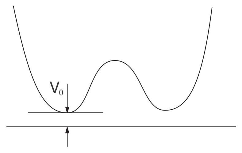
Figure 2: The Higgs potential.

Thus, here the vacuum energy itself is the cosmological constant. The constant in Eq. (5) is viewed as the contribution from the Higgs potential. Since this Veltman’s observationccp , the cosmological constant became the most difficult hierarchy problem in particle physics. As seen above, from the action it is quite natural to allow a cosmological constant. One may not prefer to choose a flat universe as a boundary condition for the equation of motion, but prefers the theory itself to choose a flat universe out of numerous possibilities. It seems that the logic for introducing a cosmological constant from the action is more fundamental than Einstein’s reasoning for a static universe.

The Einstein equation can be solved with the ansatze of a flat universe, a de Sitter space universe, or an anti de Sitter space universe. If a solution exists for a flat ansatz, then it gives a vanishing cosmological constant. If a solution exists for a de Sitter space ansatz, then it gives a positive cosmological constant, etc. It is like solving the equation of motion to seek the minimum of the potential. Note that in 4D for a nonzero cosmological constant, a flat space solution is not possible. To have a flat universe in a 4D theory, one must fine-tune $\Lambda$ at zero, which is the fine-tuning problem of the cosmological constant.

But our 4D may come from higher dimensions. In a higher dimensional theory, e.g. in 5D, we have a 5D cosmological constant. But we live in 4D, and it is perfectly allowable if the effective cosmological constant to a 4D observer is zero. In this regards, the Randall-Sundrum modelsrs1 ; rs2 are very interesting. These models start with a negative 5D cosmological constant $\Lambda_{b}$, but look for 4D flat solutions,

$$ds^{2}=\beta(y)^{2}(-dt^{2}+d{\bf x}^{2})+dy^{2}$$ (7)

where $y$ is the fifth coordinate and $\beta$ is called $`$warp factor’. The first question is, $``$Does this ansatz allow a solution?” For the Randall-Sundrum model II(RS-II)rs2 , we consider a 4-brane located at $y=0$. At the brane matter can be present, in particular a 4D cosmological constant or the brane tension $\Lambda_{1}$. With a $Z_{2}$ ansatz a solution for $\beta(y)$ satisfies $\beta(y)=\beta(-y)$. Indeed, these ansatze allow a solution for $\beta(y)$ which is expotentially suppressed at large $|y|$. Even if this theory is a 5D theory, the effect of the deep bulk($|y|\gg 1$) is negligible and can be considered as a good effective 4D theory after integrating out with respect to $y.$ But a flat solution is possible with the condition between parameters,

$$k_{b}=k_{1},\ \ k_{b}=\sqrt{-\frac{\Lambda_{b}}{6M^{3}}},\ \ k_{1}=\frac{\Lambda_{1}}{6M}$$ (8)

But this fine-tuning condition can be thought as an improvement compared to the 4D case since we started with an arbitrary negative bulk cosmological constant. It seems that the higher dimensional theories may lead to a solution of the cosmological constant problem.

Previously, there were several attempts toward a solution of the cosmological constant problem, notably by Hawking, Witten, Weinberg, and Coleman, under the name of probabilistic interpretation in Euclidian quantum gravityhawking , boundary of different phaseswitten , anthropic solutionweinberg1 , and wormholescoleman . For example, the argument of anthropic principle is the following. Life evolution is not very much affected by the existence of the cosmological constant. But galaxy formation may be hindered if the cosmological constant is too large. Weinberg obtained a bound for the condensation of matter: $\rho<550\rho_{c}$ where $\rho_{c}$ is the critical energy density. In this case, one needs a fine-tuning of 1 out of 1000, which is a big improvement. The anthropic solution seems to work. But the anthropic solution needs a multi universe scenario so that out of multiple universes, somewhere the hospitable universe may exist.

In this talk, I review the self-tuning solution. I distinguish the earlier version and the recent version.

Weak self-tuning solution

If a solution for the flat space exists in the given theory, then it is called the self-tuning solution or the undetermined integration constant solution. For a specific value of the undetermined integration constant $c$, a flat space is possible. For example, Witten used the field strength $H_{\mu\nu\rho\sigma}$ of third rank antisymmetric tensor field. In this case, indeed there is an undetermined integration constant $c$, and the vacuum energy is proportional to $c^{2}$. This undetermined integration constant can be chosen to make the space flat. Wittenwitten argued that probably the boundary of different phases is chosen. The flat space is the boundary of the de Sitter and anti de Sitter spaces. However, once $c$ is determined, there is no more free parameter to adjust when a phase transition adds a further vacuum energy. So in 4D this does not work, which has the root that $H_{\mu\nu\rho\sigma}$ is not a dynamical field in 4D. Hawking used the same field but his argument is a probabilistic one in Euclidian quantum gravity. We will discuss more about Hawking’s idea later.

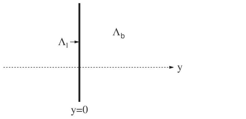
Figure 3: The RS-II model.

Strong self-tuning solution

As seen above, the weak self-tuning solution does not care whether there exist de Sitter or anti de Sitter space solutions. Choosing the flat space solution came from another principle. Recently, a more restricted class of self-tuning solutions have been attemptedkachru . It requires that there is no de Sitter and anti de Sitter space solutions except the flat one. Recently, this strong self-tuning solution has attracted a great deal of attention. In particular, the RS type modelsrs1 ; rs2 ; GB , using a negative but nonzero bulk cosmological constant and nonzero brane tension(s), allow 4D flat space solutions with fine-tuning(s). Therefore, the RS models is a good playground for the self-tuning solutions, starting with non-vanishing 5D vacuum parameters.

Firstly, let us observe the key points of the RS type models in terms of the RS-II model. The RS-IIrs2 model is an alternative to compactification. The fifth dimension $y$ is not compactified, but one can obtain an effective 4D theory due to the localization of gravity near $y=0$. It can be studied with the following 5D Lagrangian,

$${\cal L}=\frac{M^{3}}{2}(R-\Lambda_{b})+({\cal L}_{\rm matter}-\Lambda_{1})\delta(y)$$ (9)

where $M$ is the 5D fundamental scale, $\Lambda_{b}$ is the bulk cosmological constant, and $\Lambda_{1}$ is the brane tension. It is depicted in Fig. 3.

With the flat space ansatz, $ds^{2}=\beta(y)\eta_{\mu\nu}x^{\mu}x^{\nu}+dy^{2}$, one can obtain a solution

$$\beta(y)=\beta_{0}e^{-k|y|},\ \ \ k=\sqrt{-\frac{\Lambda_{b}}{6M^{3}}}.$$ (10)

Thus, only the AdS bulk allows the solution. If there are more branes, there are more conditions to satisfy toward a flat space solution since there are more brane tensions. Thus, the RS-II model is the easiest one(with only one brane tension) for a self-tuning solution.

The strong self-tuning solution attracted a great deal of interest because of a possibility to realize such a schemekachru . They tried a Lagrangian with a dilaton-like field $\phi$,

$${\cal L}=R-\Lambda^{a\phi}-\frac{4}{3}(\nabla\phi)^{2}-Ve^{b\phi}\delta(y),$$ (11)

where $a,V,$ and $b$ are constants. We set $M^{3}/2=1.$ It is a RS-II type model with a massless scalar field in the bulk. This scalar $\phi$ interacts with the brane tension. The relevant equations of motion are

$${\rm dilation}\ : \frac{8}{3}\phi^{\prime\prime}+\frac{32}{3}A^{\prime}\phi^{\prime}-a\Lambda e^{a\phi}-bV\delta(y)e^{b\phi}=0$$ (12)

$${\rm(55)\ component}\ : 6(A^{\prime})^{2}-\frac{2}{3}(\phi^{\prime})^{2}+\frac{1}{2}\Lambda e^{a\phi}=0$$ (13)

$${\rm(55),}\ (\mu\nu)\ : 3A^{\prime\prime}+\frac{4}{3}(\phi^{\prime})^{2}+\frac{1}{2}e^{b\phi}V\delta(y)=0$$ (14)

where $A=\frac{1}{2}\ln\beta(y)$ is the metric part with the 4D flat space ansatz. Indeed, one can find a solution with this flat space ansatz, for the relations $A^{\prime}=\alpha\phi^{\prime}$ and $\Lambda=0$. The solution is

$$\phi=\pm\frac{3}{4}\ln|\frac{4}{3}y+c|+d,\ \ \mbox{for the case of }\alpha=\pm\frac{1}{3}.$$ (16)

There are two types for this function: one without singularity and the other with a singularity at $y_{c}\equiv-\frac{3}{4}c$. The non-singluar solution diverges logarithmically at large $|y|$ and hence the localization of gravity near the brane is not realized. For the singular solution, the singular point $y_{c}$ is the naked singularity. But we cannot ignore the space $|y|>y_{c}$. Even if the bulk for a given $y$ is a flat 4D, the effective theory must know the whole $y$ space, including the boundary term if such a term is present. In either case, the solution is not complete. For the non-singular solution F$\ddot{\rm o}$rste et al.nilles tried to cure the singularity by inserting another brane at $y=y_{c}$. Then a flat 4D solution is possible. But there must be one fine-tuning. One more brane introduces one more parameter(the brane tension), and for a specific value of this additional brane tension the space is flat. Certainly, for another value for this tension the solution is not flat. Therefore, it is fair to say that we have not obtained a strong self-tuning solution yet.

A weak self-tuning solution with $1/H^{2}$

For a self-tuning solution, it is a necessity to introduce additional fields. In the RS-II model, one can guess that it is better to introduce a massless scalar field since it must affect the whole bulk. Indeed, Kachru et al.kachru tried a massless bulk scalar. It may be better if this massless scalar arises from the symmetry argument. Indeed, in $(4+n)$ space-time an antisymmetric tensor gauge field with $(2+n)$ indices gives a massless scalar. Therefore, in 5D RS-II type models, let us introduce $A_{MNP},\ (M,N,P=0,1,2,3,5)$. Its field strength is a 4-form field $H_{MNPQ}$. Under the gauge transformation

$$A_{MNP}\rightarrow A_{MNP}+\partial_{[M}\lambda_{NP]},$$

the 4-form field $H$ is invariant. There will remain a $U(1)$ gauge symmetry(but in fact global since there is only one component of the dynamical field) with one massless pseudoscalar $a$, $\partial_{M}a\propto\epsilon_{MNPQR}H^{NPQR}$. It remains to be seen whether there exists a self-tuning solution.

Let us consider the simplest kinetic energy term,

$$S=\int d^{5}x\sqrt{-G}\left[\frac{M^{3}}{2}R-\frac{M}{2\cdot 4!}H^{2}-\Lambda_{b}\right]+\int d^{4}x\sqrt{-g}(-\Lambda_{1})$$ (17)

where $H^{2}=H_{MNPQ}H^{MNPQ}$, and $G$ and $g$ are the determinants of the 5D and 4D metrics, respectively. The brane with the brane tension $\Lambda_{1}$ is located at $y=0$. We have the following ansatz,

Flat 4D $$: \ ds^{2}=\beta(y)^{2}\eta_{\mu\nu}dx^{\mu}dx^{\nu}+dy^{2}$$ (18)

4D chosen $$: H_{\mu\nu\rho\sigma}=\frac{\epsilon_{\mu\nu\rho\sigma}}{\sqrt{-G}n(y)}$$ (19)

where $\mu,\cdots,$ are the 4D indices. In the remainder of this talk we work with the unit system $M=1$ unless the parameter is explicitly inserted. The $H$ equation, the (55) and $(\mu\nu)$ component Einstein equations are solved to give the following solutions:

$$\Lambda_{b}<0 : \beta(|y|)=(a/k)^{1/4}[\pm\sinh(4k|y|+c)]^{1/4}$$ (20)

$$\Lambda_{b}>0 : \beta(|y|)=(a/k)^{1/4}[\sin(4k|y|+c^{\prime})]^{1/4}$$ (21)

$$\Lambda_{b}=0 : \beta(|y|)=[|4a|y|+c^{\prime\prime}|]^{1/4}$$ (22)

For a localizable(near $y=0$) metric, there exists a singularity at $|y|=-c/4k,$ etc. Thus another brane is necessary and needs a fine-tuning. We encounter a similar problem as in the case of Kachru et al.kachru . It is worth commenting the de Sitter space solution, for $\Lambda_{b}>0$. It is a periodic solution as shown in Fig. 4.

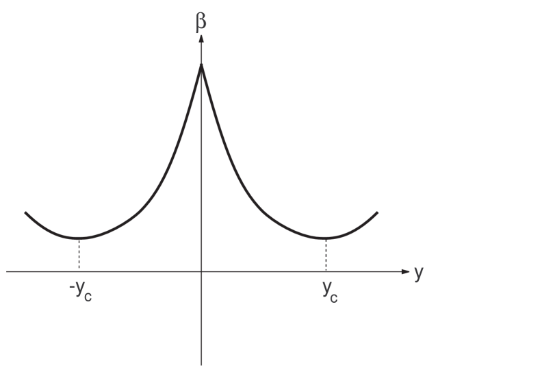
Figure 4: The solution with $H^{2}$ in the bulk de Sitter space.

Since $\beta^{\prime}=0$ at $y=\pm y_{c}$, we can restrict to the subspace $|y|\leq y_{c}$. Then the boundary conditions at $y=0$ and $y_{c}$ relate the parameters

$$c=\cot^{-1}(k_{1}/k),\ \ \ c=4ky_{c}-\cot^{-1}(k^{2}/k),$$

where $c$ is an integration constant determined by the brane tension and the bulk cosmological constant. Then, if $y_{c}$ behaves like an undetermined integration constant, we can achieve a self-tuning solution. But $y_{c}$ is the vacuum expectation value(VEV) of the radion field $g_{55}$ which cannot be a strictly massless Goldstone boson. If it were massless, it will serve to the long range gravitational interaction and hence give a different result from the prediction of the Einstein gravity for the light bending experiments. It will obtain mass, and hence $y_{c}$ is not a free parameter but is fixed. Then the second equation is nothing but a fine-tuning conditionlee1 .

But we find a self-tuning solution with $1/H^{2}$kkl . We present this solution here, not because it has a meaningful kinetic energy term but because to show that there exists a solution. At low energy, we may treat it as an effective interaction term. Setting $M=1$, the action is

$$S=\int d^{4}x\int dy\left[\frac{1}{2}R+\frac{2\cdot 4!}{H^{2}}-\Lambda_{b}-\Lambda_{1}\delta(y)\right]$$ (23)

where $-\Lambda_{1}$ can be interpreted as the VEV of the matter Lagrangian at the brane. At low energy, this Lagrangian makes sense only if $H^{2}$ develops a VEV. Again, we impose the following ansatze

Flat 4D $$: \ ds^{2}=\beta(y)^{2}\eta_{\mu\nu}dx^{\mu}dx^{\nu}+dy^{2}$$ (24)

4D chosen $$: H_{\mu\nu\rho\sigma}=\frac{\sqrt{-g}\epsilon_{\mu\nu\rho\sigma}}{n(y)}$$ (25)

$$\ H_{5\mu\nu\rho}=0.$$ (26)

The $H$ field equation is $\partial_{M}[\sqrt{-g}H^{MNPQ}/H^{4}]=\partial_{\mu}[\sqrt{-g}H^{\mu NPQ}/H^{4}]=0.$ Thus, we conclude $n$ is a function of $y$ only. For simplicity, we require a $Z_{2}$ symmetry the symmetry under the reflection: $y\rightarrow-y$. The bulk solution iskkl

$$\beta(|y|)=\left[\frac{(k/a)}{\cosh(4k|y|+c)}\right]^{1/4}$$ (27)

where $a$ and $c$ are the integration constants, and

$$k=\sqrt{-\frac{\Lambda_{b}}{6}},\ \ k_{1}=\frac{\Lambda_{1}}{6}.$$ (28)

The boundary condition at $y=0$ is

$$\left.\frac{\beta^{\prime}}{\beta}\right|_{0^{+}}=-\frac{\Lambda_{1}}{6}.$$ (29)

The bulk solution (27) has the integration constants $a$ and $c$. $a$ is basically the global charge of the universe and determines the finite 4D Planck mass. $c$ is the undetermined integration constant we want and is fixed by the boundary condition at $y=0$ without fine-tuning, for a finite range of $|\Lambda_{1}|<\sqrt{-\Lambda_{b}/6}$,

$$\tanh c=\frac{k_{1}}{k}=\frac{\Lambda_{1}}{\sqrt{-6\Lambda_{b}}}.$$ (30)

Since changing $c$ amounts to changing the fields, if the value $\Lambda_{1}$ is changed then the fields are expected to adjust so that the flat space solution results. Note that $\beta(|y|)$ is a decreasing function of $|y|$ and converges to 0 exponentially as $|y|\rightarrow\infty$. This property is needed for a self-tuning solution.

The key points of our solution are:

(1) $\beta$ has no naked singularity–If we obtain a 4D flat solution at every bulk point $y$, then the effective 4D cosmological constant must be zero since there is no singularity.

(2) 4D Planck mass is finite–Even if the extra dimension is not compact, this theory is permissible since the gravity is localized near the brane. Integrating with respect to $y$, we obtain an effective 4D Planck mass

$$M^{2}_{\rm 4D\ Planck}=\int\sqrt{\beta^{4}}dy=2M^{3}\sqrt{\frac{k}{a}}\int_{0}^{\infty}\frac{1}{\sqrt{\cosh(4ky+c)}}dy$$ (31)

which is finite and is expected to be of order $M^{2}$ if the bulk cosmological constant and the brane tension are of that scale.

(3) It is a self-tuning solution–To see that the 4D cosmological constant is zero, we must also consider the surface termkkl ,

$$S_{\rm surface}=\int d^{4}xdy\ 4\cdot 4!\left[\frac{\sqrt{-g}}{H^{2}}+A_{NPQ}\partial_{M}\left(\frac{\sqrt{-g}H^{MNPQ}}{2H^{4}}\right)\right].$$ (32)

Thus, the total action is

$$S=\int d^{4}xdy\ \sqrt{-\eta}\beta^{4}\left[\frac{R_{4}}{2\beta^{2}}-4\frac{\beta^{\prime\prime}}{\beta}-6\left(\frac{\beta^{\prime}}{\beta}\right)^{2}-\Lambda_{b}+\frac{2\cdot 4!}{H^{2}}-\Lambda_{1}\delta(y)\right]+S_{\rm surface}.$$ (33)

Then, $-\Lambda_{\rm eff}$ is the $y$ integral of Eq. (33) except the 4D Einstein-Hilbert term $R_{4}$, to give vanishing cosmological constantkkl . It is consistent with the original flat 4D ansatz.

Therefore, we obtained a flat space solution with $1/H^{2}$ term. Certainly, the theory we consider does not belong to the class studied for the no go theorem, without the Gauss-Bonnet termcsaki and with the Gauss-Bonnet termzee . [Note added: After this talk, more self-tuning solutions were found with a general function of $H^{2}$ lee and with the Gauss-Bonnet termbinetruy . With the Gauss-Bonnet term, there is a new class of solutions which does not include the RS pointGB . The solution obtained by Binetruy et al. belongs to the class not containing the RS model, or more accurately to the class containing the Kachru et al. pointkachru .]

Note that our solution needs a bulk massless scalar. Namely, only derivative terms are needed in the bulk, which reminds us of a Goldstone boson. Another point is that the kinetic energy term is not a standard one, $1/H^{2}$. In fact, there are more solutions with non-standard kinetic energy termskkl ; lee , but the solution we presented is expressed in a closed form and hence is transparent for discussing the resulting physics.

Dual description

In the dual picture, we have a 5D scalar $\sigma$. The dual relation isckl

$$H_{MNPQ}=\sqrt{-g}\epsilon_{MNPQR}\frac{\partial^{R}\sigma}{(4!)^{1/3}[(\partial\sigma)^{2}]^{2/3}}.$$ (34)

In this dual picture, we obtain the same warp factor with the self-tuning property. The kinetic energy term of $\sigma$ is

$$-[(\partial\sigma)^{2}]^{2/3}$$ (35)

which is not standard. The equation of motion of $H$ becomes the Bianchi identity in the dual picture, and the Bianchi identity plays the role of equation of motion in the dual pictureckl . In the dual picture, we can allow the brane coupling,

$$-\Lambda_{1}f(\sigma)\delta(y)$$ (36)

which may be useful for further study of self-tuning solutions.

De Sitter and anti de Sitter space solutions

So far we have considered the time-independent solutions. The next simplest solutions are de Sitter and anti de Sitter space solutions which are time dependent. For the curvature $\lambda$($+$ sign for dS and $-$ sign for AdS), the metric is taken as

$$ds^{2}=\beta^{2}(y){\bf g}_{\mu\nu}dx^{\mu}dx^{\nu}+dy^{2}$$ (37)

where

$${\bf g}_{\mu\nu}=\left\{\matrix{{\rm diag.}(-1,e^{2\sqrt{\lambda}t},e^{2\sqrt{\lambda}t},e^{2\sqrt{\lambda}t}),\ \ \mbox{for dS}_{4}\cr{\rm diag.}(-e^{2\sqrt{-\lambda}x_{3}},e^{2\sqrt{-\lambda}x_{3}},e^{2\sqrt{-\lambda}x_{3}},1),\ \ \mbox{for AdS}_{4}\cr}\right.$$ (38)

The 4D Riemann tensor is $R_{\mu\nu}=3\lambda{\bf g}_{\mu\nu}$. Thus, the (55) and (00) component equations are

$$6(\beta^{\prime}/\beta)^{2}-6\lambda\beta^{-2}=-\Lambda_{b}-3(\beta^{8}/A)$$ (39)

$$3(\beta^{\prime}/\beta)^{2}+3(\beta"/\beta)-3\lambda\beta^{-2}=-\Lambda_{b}-\Lambda_{1}\delta(y)-3(\beta^{8}/A)$$ (40)

The 4D cosmological constant obtained from the above ansatz should be $\lambda$. But we cannot show this explicitly since we do not have an exact solution. Nevertheless, this kind of situation can be checked from the Karch-Randall(KR) solution with the fine-tuning ansatzkarch . For the dS solution,

$$\beta(y)=(\sqrt{\lambda}/k)\sinh[k(y_{m}-y)],\ \ y_{m}=(1/k)\coth^{-1}(k_{1}/k),$$ (41)

the effective Planck mass and the effective cosmological constant are obtained by integrating in $[-y_{m},y_{m}],$

$$M^{2}_{P,{\rm eff}}=(\lambda/k^{3})(-ky_{m}+\frac{1}{2}\sinh(2ky_{m}))>0$$ (42)

$$\Lambda_{\rm eff}=(\lambda^{2}/k^{3})(-ky_{m}+\frac{1}{2}\sinh(2ky_{m}))=\lambda M^{2}_{P,{\rm eff}}.$$ (43)

Therefore, a 4D observer would realize the curvature as $\lambda$. Similarly, we expect that for our dS and AdS solutions, the 4D curvature will turn out to be $\lambda$. Our solutions are depicted in Figs. 5, 6, and 7.

Figure 5: The flat space solution.

Figure 6: The de Sitter space solution.

Figure 7: The anti de Sitter space solution.

It is easy to observe that these solutions exist. The $y$ derivative of the metric for the dS case is

$$\beta^{\prime}=\sqrt{k_{\lambda}^{2}+k^{2}\beta^{2}-a^{2}\beta^{10}},\ \ {\rm with}\ k_{\lambda}=\sqrt{\lambda/6}.$$ (44)

Therefore, for a positive $\lambda$, $\beta^{\prime}(y_{h})$ needs not be zero at the point where $\beta(y_{h})=0$. Thus, there exist a point $y_{h}$ where $\beta^{\prime}$ is finite and $\beta=0$ which is the de Sitter horizon. It takes an infinite amount of time to reach at $y_{h}$. For a negative $\lambda$, $\beta$ can be nonzero where $\beta^{\prime}$ is zero. It is an AdS solution, which does not give a localized gravity.

Probabilistic interpretation

We note that in 4D with $\Lambda\neq 0$, a flat solution is not possible. In our case, we obtained flat, dS₄, and AdS₄ solutions for a finite range of parameters. It is a progress, since one can choose the flat one if there exists a principle to do sohawking ; witten . In particular, let us briefly review Hawking’s idea in 4D. In the Euclidian quantum gravity, the Euclidian action is

$$-S_{E}=-\frac{1}{2}\int d^{4}x\sqrt{+g}[(R+2\Lambda)+\frac{1}{4!}H_{\mu\nu\rho\sigma}H^{\mu\nu\rho\sigma}],$$ (45)

where we used the gravity unit $M^{2}=1$. The Einstein and $H$ equations are

$$R_{\mu\nu}-\frac{1}{2}g_{\mu\nu}R=\Lambda g_{\mu\nu}-T_{\mu\nu}$$ (46)

$$\partial_{\mu}[\sqrt{g}H_{\mu\nu\rho\sigma}]=0$$ (47)

where

$$H_{\mu\nu\rho\sigma}=\frac{1}{\sqrt{g}}\epsilon_{\mu\nu\rho\sigma}c,\ \ H^{2}=4!c^{2},\ \ T_{\mu\nu}=\frac{1}{6}H_{\mu abc}H_{\nu abc}-\frac{1}{48}g_{\mu\nu}H^{2}$$ (48)

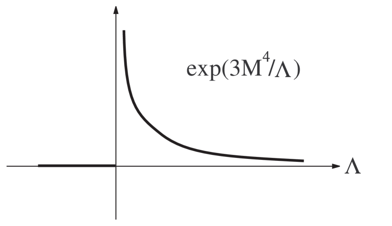
Figure 8: Hawking’s probability function.

Thus, we obtain $T_{\mu\nu}=\frac{1}{2}c^{2}g_{\mu\nu}=-\Lambda_{H}g_{\mu\nu}$ where $\Lambda_{H}=-\frac{1}{2}c^{2}$. The Ricci scalar is

$$R=-g_{\mu\nu}(R_{\mu\nu}-\frac{1}{2}g_{\mu\nu}R)=-4\Lambda_{\rm eff}$$ (49)

where

$$\Lambda_{eff}=\Lambda+\Lambda_{H}.$$ (50)

We obtained (49) from the equation of motion, but not from the action itself. If we used the action, then we had to include the surface term. Therefore, consider for $\Lambda_{\rm eff}>0$,

$$-S_{E}=-\frac{1}{2}\int d^{4}x\sqrt{g}(R+2\Lambda_{\rm eff})=\int d^{4}x\sqrt{g}\Lambda_{\rm eff}$$ (51)

$$=\Lambda_{\rm eff}\cdot\mbox{(4D Euclidian volume)}=\frac{3M^{4}}{\Lambda_{\rm eff}}$$ (52)

which is maximum at $\Lambda_{\rm eff}=0^{+}$, which is shown in Fig. 8.

Therefore, Hawking interpreted this result as the probability for the $\Lambda_{\rm eff}=0^{+}$ universe is maximum in the multi universe scenario. As explained in the introduction, this 4D example is not realistic since the universe is originating from Big Bang where the beginning of time chooses the universe. This Hawking’s argument applies at the beginning. But at later epoches, the vacuum energies are expected to be added and hence the 4D example is not complete.

With our self-tuning solution, we can anticipate that one can choose the flat one in the beginning after inflation and at a later epoch the flat solution adjusts itself if vacuum energy is added at the brane.

In conclusion, we presented the interesting self-tuning solutions of the cosmological constant problem, which has attracted a great interest recently. This direction seems to be promising in RS-II type models. We showed an existence proof of such a solution with the four-form field strength $H$ in 5D. To choose the flat one out of numerous possibilities, we had to resort to Hawking’s probabilistic interpretation. But there may be some theories where these strong self-tuning solutions are possible. To find these new type of solutions, it is worthwhile to observe the key points of our solutions and presumably one may rely on a symmetry in theories with a massless scalar coupled to the brane.

Acknowledgments: This work is supported in part by the BK21 program of Ministry of Education and by the KOSEF Sundo grant.

References

- (1) E. Gildener and S. Weinberg, Phys. Rev. D13, 3333 (1976).
- (2) M. Veltman, Phys. Rev. Lett. 34, 777 (1975). For earlier discussions, refer to Ya. B. Zel’dovich and I. D. Novikov, Relativistic Astrophysics, Vol. I (1967 Russian ed., English Translation in 1971, Univ. of Chicago Press), p.72; Vol. II (Univ. of Chicago Press, 1983), Chapter 4. For a recent summary, see, U. Ellwanger, hep-ph/0203252.
- (3) R. D. Peccei and H. R. Quinn, Phys. Rev. Lett. 38, 1440 (1977).
- (4) J. E. Kim and H. P. Nilles, Phys. Lett. B138, 150 (1984).
- (5) S. Weinberg, Rev. Mod. Phys. 61, 1 (1989).
- (6) S. Hawking, Phys. Lett. B134, 403 (1984); E. Baum, Phys. Lett. B138, 185 (1983).
- (7) E. Witten, Proc. Shelter Island II Conference(Shelter Island, 1983), ed. R. Jackiw, H. Khuri, S. Weinberg, and E. Witten (MIT Press, 1985), p.369. was used also by A. Aurila, H. Nicolai, and P. K. Townsend, Nucl. Phys. B176, 509 (1980).
- (8) S. Weinberg, Phys. Rev. Lett. 59, 2607 (1987).
- (9) S. Coleman, Nucl. Phys. B310, 643 (1988).
- (10) Ya. B. Zel’dovich and I. D. Novikov, Relativistic Astrophysics, Vol. I (1967 Russian ed., English Translation in 1971, Univ. of Chicago Press), p.72; Vol. II (Univ. of Chicago Press, 1983), Chapter 4.
- (11) S. Perlmutter et al., The Supernova Cosmology Project, Bull. Am. Astron. Soc. 5, 1351 (1998).
- (12) For an extremely light light Goldstone boson as quintessence, see, J. E. Kim, JHEP 9905, 022 (1999); JHEP 0006, 016 (2000); K. Choi, Phys. Rev. D62, 043509 (2000). For other types, see, P. Binetruy, Phys. Rev. D60, 063502 (1999); C. Kolda and D. H. Lyth, Phys. Lett. B458, 197 (1999); T. Chiba, Phys. Rev. D60, 083508 (1999); P. Brax and J. Martin, Phys. Lett. B468, 40 (1999); A. Masiero, M. Pietroni, and F. Rosati, Phys. Rev. D61, 023504 (2000); M. C. Bento and O. Bertolami, Gen. Rel. Grav. 31, 1461 (1999); F. Perrotta, C. Baccigalupi, and M. Matarrese, Phys. Rev. D61, 023507 (2000).
- (13) L. Randall and R. Sundrum, Phys. Rev. Lett. 83, 3370 (1999).
- (14) L. Randall and R. Sundrum, Phys. Rev. Lett. 83, 4690 (1999).
- (15) N. Arkani-Hamed, S. Dimopoulos, N. Kaloper, and R. Sundrum, Phys. Lett. B480, 193 (2000); S. Kachru, M. Schulz, and E. Silverstein, Phys. Rev. D62, 045021 (2000).
- (16) J. E. Kim, H. M. Lee, and B. Kyae, Phys. Rev. D62, 045013 (2000); Nucl. Phys. B582, 296 (2000).
- (17) S. Frste, Z. Lalak, S. Lavignac, and H. P. Nilles, JHEP 0009, 034 (2000).
- (18) J. E. Kim, B. Kyae, and H. M. Lee, hep-th/0110103.
- (19) J. E. Kim, B. Kyae, and H. M. Lee, Phys. Rev. Lett. 86, 4223 (1991); Nucl. Phys. B613, 306 (2001).
- (20) C. Csaki, J. Erlich, C. Grojean, and T. Hollowood, Nucl. Phys. B584, 359 (2001).
- (21) I. Low and A. Zee, Nucl. Phys. B585, 395 (2000).
- (22) J. E. Kim and H. M. Lee, hep-th/0207260.
- (23) P. Binetruy, C. Charmousis, S. C. Davis, and J.-F. Dufaux, hep-th/0206089.
- (24) K.-S. Choi, J. E. Kim, and H. M. Lee, J. Korean Phys. Soc., 40, 207 (2002) [hep-th/0201055].
- (25) A. Karch and L. Randall, JHEP 0105, 008 (2001).