CERN-TH/2002-169

NSF-ITP-02-43

FINITE TEMPERATURE Z($N$) PHASE TRANSITION
WITH KALUZA-KLEIN GAUGE FIELDS

K. Farakos^a,, P. de Forcrand^b,c,, C.P. Korthals Altes^d,c,,
M. Laine^c,e,, and M. Vettorazzo^b,

^aPhysics Department, NTU, 15780 Zografou Campus, Athens, Greece

^bInstitut für Theoretische Physik, ETH Zürich, CH-8093 Zürich, Switzerland

^cTheory Division, CERN, CH-1211 Geneva 23, Switzerland

^dCentre Physique Théorique, CNRS, Case 907, Luminy, F-13288 Marseille, France

^eITP, University of California, Santa Barbara, CA 93106-4030, USA

If SU($N$) gauge fields live in a world with a circular extra dimension, coupling there only to adjointly charged matter, the system possesses a global Z($N$) symmetry. If the radius is small enough such that dimensional reduction takes place, this symmetry is spontaneously broken. It turns out that its fate at high temperatures is not easily decided with straightforward perturbation theory. Utilising non-perturbative lattice simulations, we demonstrate here that the symmetry does get restored at a certain temperature $T_{c}$, both for a 3+1 and a 4+1 dimensional world (the latter with a finite cutoff). To avoid a cosmological domain wall problem, such models would thus be allowed only if the reheating temperature after inflation is below $T_{c}$. We also comment on the robustness of this phenomenon with respect to small modifications of the model.

CERN-TH/2002-169
NSF-ITP-02-43
December 2002

1 Introduction

It has recently been suggested that new venues for, e.g., Grand Unification, could be obtained by considering compact extra dimensions of an inverse radius at the TeV scale, with non-Abelian gauge fields propagating in the bulk (see, e.g., [1, 2, 3] and references therein).

It is well known that if SU($N$) gauge fields were to couple only to adjointly charged matter, and the radius of a compact circular dimension is such that a weak coupling computation is reliable, then the system possesses a spontaneously broken global Z($N$) symmetry, related to the Polyakov loop in the extra direction [4, 5, 6, 7]. This leads to the existence of topological domain wall defects [8, 9, 10, 11].

Of course, such domain walls would carry a huge energy density, $\sim$TeV³, and could thus not be produced under any normal circumstances. However, if the symmetry gets restored at a high temperature $T_{c}$, domain walls could possibly be produced in a cosmological phase transition in the Early Universe. On the other hand, the existence of domain walls with energy densities exceeding about MeV³ can be excluded experimentally, for instance, through the anisotropies in the cosmic microwave background radiation [12, 13]. This means that either particle physics models of this type are not realised in nature or, in analogy with how the monopole problem can be avoided in the case of traditional grand unified theories, the cosmological history is such that the reheating temperature after inflation is sufficiently below $T_{c}$.

Given the meaningful conclusions that can be drawn, it seems worthwhile to ask whether there really is a symmetry restoring phase transition in these models. This is not automatically guaranteed to be the case [14]: there are even non-perturbatively established examples of broken symmetries which do not get restored at high temperatures [15]. Then one would obviously have no domain wall problem [16].

It turns out that in the present context the issue cannot easily be solved with perturbation theory, since it breaks down close to the phase transition point [18]. On the other hand, various non-perturbative arguments suggest that the symmetry should get restored [18]. Here we confirm the latter arguments with lattice simulations.

The model we study is pure SU(2) gauge theory. We take it to live either in four Euclidean dimensions (4d), standing for one time direction, two space directions, and one compact extra dimension — or in five dimensions (5d), standing for one time direction, three space directions, and one compact extra dimension. A continuum limit can only be approached in 4d, since a 5d pure Yang-Mills theory is not renormalisable. Nevertheless, for a fixed lattice spacing, the qualitative features of the phase diagram can be addressed also in the 5d case.

In Sec. 2 we specify the lattice model studied, as well as the observables measured. We present our 4d data in Sec. 3, our 5d data in Sec. 4, and conclusions in Sec. 5.

2 Basic formulation

2.1 Lattice action and observables

We denote the number of dimensions by $d$, $d=4,5$. Two of the dimensions are assumed compact and periodic: a time direction $\tau=0...L_{\tau}$, where $T=L_{\tau}^{-1}$ is the temperature, and a compact spatial dimension $y=0...L_{y}$, where $M\equiv L_{y}^{-1}$. The lengths of the remaining (in principle infinite) dimensions are denoted by $L_{i}$, $i=1,...,d-2$.

We regularise the theory by introducing a spacetime lattice, with a lattice spacing $a$. The lattice spacing is taken the same in all directions. We denote $L_{\tau}=aN_{\tau}$, $L_{y}=aN_{y}$, $L_{i}=aN_{i}$. The lattice action is of the standard Wilson form,

$$S = \beta_{G}\sum_{x}\sum_{\mu<\nu}\Bigl{(}1-{\frac{1}{2}}{\rm Tr\,}P_{\mu\nu}\Bigr{)},$$ (2.1)

where $P_{\mu\nu}$ is an SU(2) plaquette, and $\mu,\nu=1,...,d$. The (dimensionless) value of $\beta_{G}$ determines the lattice spacing $a$; we return to the conversion in Sec. 3.4.

Our aim, from the point of view of the discretised theory, is to determine the phase diagram of the system in the three-dimensional space spanned by $\beta_{G},N_{\tau},N_{y}$. The spatial volume $V\equiv L_{1}L_{2}...L_{d-2}$ is assumed extrapolated to infinity.

The observables we employ in order to determine the phase diagram are the Polyakov loops in the $\tau$ and $y$ directions,

$$P_{\tau}(x_{i},y) = {\frac{1}{2}}{\rm Tr\,}\prod_{n=0}^{N_{\tau}-1}U_{\tau}(x+n\hat{\tau}),$$ (2.2)

$$P_{y}(x_{i},\tau) = {\frac{1}{2}}{\rm Tr\,}\prod_{n=0}^{N_{y}-1}U_{y}(x+n\hat{y}),$$ (2.3)

where the $U_{\tau},U_{y}$ are link matrices, $x=(x_{i},\tau,y)$, $i=1,...,d-2$, and $\hat{\tau}$, $\hat{y}$ are unit vectors in the directions of $\tau,y$. We also monitor the plaquette, $\langle{\rm Tr\,}P_{\mu\nu}(x)\rangle$.

For both observables we measure the distribution of their volume average,

$$\bar{P}_{\tau}\equiv\frac{a^{d-1}}{VL_{y}}\sum_{x_{i},y}P_{\tau}(x_{i},y),\quad\bar{P}_{y}\equiv\frac{a^{d-1}}{VL_{\tau}}\sum_{x_{i},\tau}P_{y}(x_{i},\tau).$$ (2.4)

Let us define, in particular,

$$|P_{\tau}|\equiv\langle\,|\bar{P}_{\tau}|\,\rangle\,,\quad\chi(P_{\tau})\equiv\frac{VL_{y}}{a^{d-1}}\Bigl{[}\langle\,(\bar{P}_{\tau})^{2}\,\rangle-\langle\,|\bar{P}_{\tau}|\,\rangle^{2}\Bigr{]}\,,$$ (2.5)

and in complete analogy for $|P_{y}|,\chi(P_{y})$. Physically, the role of $|P_{y}|$ is to tell whether dimensional reduction into a $d-1$ dimensional effective theory takes place ($|P_{y}|>0$) or not ($|P_{y}|=0$), while the role of $|P_{\tau}|$ is to tell whether the effective $d-1$ dimensional theory is confining ($|P_{\tau}|=0$) or not ($|P_{\tau}|>0$). Let us recall that here $d-1$ is supposed to comprise the $d-2$ flat physical spatial dimensions, as well as the one time dimension; for $d=4$ we are thus in effect considering a toy model of a (2+1)-dimensional world.

2.2 Universality class

As we vary $\beta_{G},N_{\tau},N_{y}$, we may expect to find phase transitions. In case the transitions turn out to be of the second order, as is mostly the case, they are associated with some universality class, which we now discuss.

We have introduced two actual order parameters for the system, ${P_{y}}$, ${P_{\tau}}$, whose phases are Z(2) variables. In the limit of $N_{\tau}\gg N_{y}$ or $N_{y}\gg N_{\tau}$, only one of them is “critical” at the transition point; then the scaling goes to a good approximation according to the Ising model in $d-1$ dimensions [19]. For comparable $N_{\tau},N_{y}$ when both can be critical, the universality class is that of the Z(2)$\times$Z(2) model in $d-2$ dimensions. The properties of this model however depend on a number of parameters, defining the relative strengths of the self-interactions of the two spins, as well as the interactions between them. In general the transition is still of the second order, but in special cases it can also be of the first order, at least for $d-2=3$ [20]. Below, we will indeed encounter first order phase transitions in the 5d case.

2.3 Perturbative predictions

Before turning to lattice results, let us also briefly review the predictions of continuum perturbation theory. The 1-loop finite temperature continuum effective potential for the phase of the Polyakov line, $P_{y}$, has been computed in [18], both for $d=4,5$. The structure of the potential is such that at zero temperature, assuming weak coupling for the given value of $M$ (say, $M\gg\Lambda_{\overline{\rm MS}}$ in the 4d case), the Z(2) symmetry related to $P_{y}$ is broken [10], such that $|P_{y}|>0$. This is consistent with the fact that the theory undergoes dimensional reduction to $d-1$ dimensions [21].

Increasing now the temperature, the potential turns out to show no sign of symmetry restoration. However, at temperatures parametrically of the order $T\sim M/g^{2}$, perturbation theory is seen to break down [18], and non-perturbative arguments can be given that the symmetry should get restored [18]. The resulting phase diagram was sketched in Fig. 2 of [18].

3 Lattice results in four dimensions

In order to study the phase diagram with lattice simulations, we shall employ various fixed values of $N_{y}$, $N_{y}=1,2,4$. In each case, we study a number of different $N_{\tau}$, and determine the phase diagram as a function of $\beta_{G}$. We plot the results in the plane ($1/N_{\tau},\beta_{G}$). For a fixed $\beta_{G}$ (fixing $a$), increasing $1/N_{\tau}$ (moving right) corresponds then to increasing the temperature, since $1/N_{\tau}=aT$.

$N_{\tau}$	$N_{y}$	$N_{1}\times N_{2}$
1,2,4	1	$16^{2}$
1…6	2	$16^{2}$
1…6	4	$12^{2},16^{2}$

Table 1: The volumes studied in the 4d case. Note that on account of the symmetry $N_{\tau}\leftrightarrow N_{y},P_{\tau}\leftrightarrow P_{y}$, some of them are effectively listed twice.

The 4d simulation points are shown in Table 1. At every $\beta_{G}$ close to a phase transition, we study five $\beta_{G}$-values more carefully, each with a statistics of 40K measurements (separated by 1 Metropolis and 6 overrelaxation sweeps). 10K sweeps are discarded for thermalization. Interpolation in $\beta_{G}$ is achieved through Ferrenberg-Swendsen reweighting [22], with jackknife error estimates. The location of the susceptibility maximum is obtained with a parabolic interpolation through the binned, reweighted data.

3.1 Existence of phase transitions

        

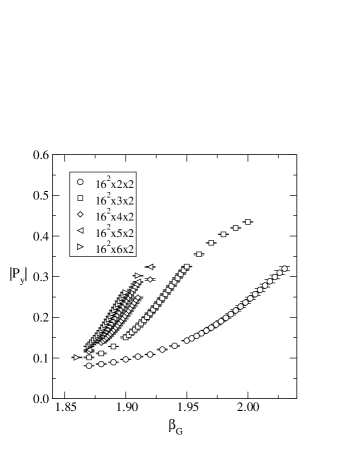
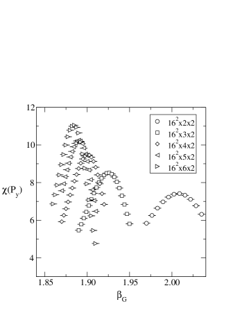
Figure 1: Left: the observable $|P_{y}|$ defined in Eq. (2.5), for $N_{y}=2$, and various $N_{\tau}$. Right: the corresponding susceptibility $\chi(P_{y})$, defined in Eq. (2.5). For $V\to\infty$, $|P_{y}|\to 0$ for $\beta_{G}$ to the left of the susceptibility maximum (cf. Figs. 5, 6).

In Fig. 1 we show the results obtained for ${|P_{y}|}$, as well as the susceptibility $\chi({P_{y}})$, as a function of $\beta_{G}$, at various $N_{\tau}$, for a fixed $N_{y}=2$. We observe that $|P_{y}|$ grows rapidly (symmetry breaks) when $\beta_{G}$ is increased beyond a certain point. The transition point is located from the maximum of $\chi(P_{y})$. We see that the location of the phase transition depends on $N_{\tau}$. Measurements of ${|P_{\tau}|}$, $\chi{(P_{\tau})}$ show similar phase transitions, however in general at some other $\beta_{G}$. By studying two different volumes for $N_{y}=4$ (Table 1), we know that the results are already representing the thermodynamic limit well enough for our purposes, as far as the position of the transition is concerned (see Fig. 2, bottom right). For $d=5$ (Sec. 4), we have carried out somewhat more extensive volume scaling tests, and they do not give rise to any concerns about our resolution.

3.2 Phase diagrams for fixed $N_{y}$

      

      

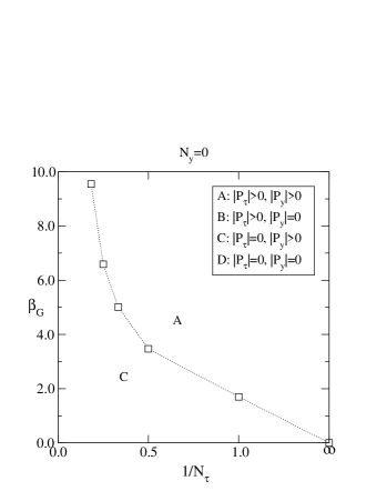
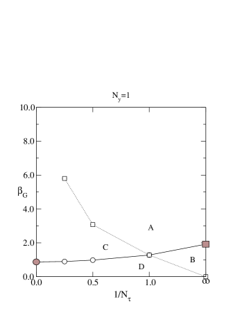
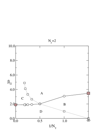
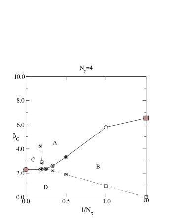
Figure 2: Phase diagrams for various $N_{y}$, in 4d. The lines connecting the simulation points are there to guide the eye only. The data for $N_{y}=0$ at $N_{\tau}\geq 2$, as well as that at $1/N_{\tau}=\infty$ (filled boxes), are from the (2+1)d studies in [23, 24], while the limiting values at $1/N_{\tau}=0$ (filled circles) are from the (3+1)d studies in [25, 26]. For $N_{y}=4$ we have shown results both at the spatial volume $12^{2}$ (small crosses) and $16^{2}$ (large open symbols), finding no appreciable volume dependence.

When results such as discussed above are collected together, we obtain the 4d phase diagrams shown in Fig. 2.

As a first check, we may compare our results with some known limits in the literature. The critical values of $\beta_{G}$ for a (2+1)d SU(2) theory at finite temperatures have been determined in [23, 24]. These results are collected in Fig. 2, top left, showing the transitions felt by ${|P_{\tau}|}$ in the limit $N_{y}=0$, but they also determine the transition points felt by ${|P_{y}|}$ at $1/N_{\tau}=\infty$ (filled boxes). The other known limit is obtained from (3+1)d at finite temperatures [25, 26]: these results fix the transitions felt by ${|P_{y}|}$ at $1/N_{\tau}=0$ (filled circles). Our data indeed interpolate between these known values.

A second check may be obtained by considering the behaviour of the transition for ${|P_{y}|}$ in the vicinity of $1/N_{\tau}=0$. Indeed, the behaviour there is sensitive to the universality class of the system. The point $1/N_{\tau}=0$ represents a (3+1)d theory, so that the transition should belong to the 3d Ising universality class. As we now move to a small $1/N_{\tau}>0$, we may expect the transition point, $\beta_{c}$, to change according to the corresponding finite-size scaling exponents. More precisely, a finite $aN_{\tau}$ acts as a length scale cutoff, so that if the correlation length $\xi$ critical exponent $\nu$ is defined as $\xi\sim|\beta-\beta_{c}|^{-\nu}$, we may expect

$$|\beta_{c}(N_{\tau})-\beta_{c}(N_{\tau}=\infty)|\approx\frac{1}{N_{\tau}^{1/\nu}}\biggr{(}c_{1}+\frac{c_{2}}{N_{\tau}^{\omega}}+...\biggl{)}.$$ (3.1)

Here we have also included $\omega$, the universal correction-to-scaling exponent. For 3d Ising, $\nu\approx 0.63$, $\omega\approx 0.8$. The results, obtained by fixing the exponents $\nu,\omega$ and fitting for $\beta_{c}(N_{\tau}=\infty),c_{1},c_{2}$, are shown in Fig. 3 for $N_{y}=2$. We find that the ansatz in Eq. (3.1) indeed allows to fit the data well, as long as $N_{\tau}\mathop{\raise 1.29167pt\hbox{$>$\kern-7.5pt\raise-4.73611pt\hbox{$\sim$}}}N_{y}$.

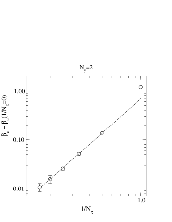
Figure 3: Finite-size scaling of the phase transition point determined from $\chi(P_{y})$ on volumes $16^{2}\times N_{\tau}\times 2$, as a function of $1/N_{\tau}$, together with a three-parameter fit according to Eq. (3.1) (fit for $\beta_{c}(N_{\tau}=\infty),c_{1},c_{2}$).

3.3 Physical implications

After these consistency checks, we draw the following physical conclusion from Fig. 2. Suppose we fix $\beta_{G}$, meaning that we fix the lattice spacing. Staying at this $\beta_{G}$ at zero temperature, $1/N_{\tau}=0$, let us increase $M$ until we are in the phase where the symmetry related to the phase of $P_{y}$ is broken (region C), by decreasing $N_{y}$ (recall that $M=1/(aN_{y})$). This effectively guarantees that dimensional reduction takes place [21]. Since $|P_{\tau}|=0$, the dimensionally reduced theory is in its confining phase. Increasing now the temperature by moving to the right ($T=1/(aN_{\tau})$), we observe that there is first a deconfinement transition to region A and then, at large enough values ($1/N_{\tau}>1/N_{y}$), we do cross the transition to the symmetric phase, $|P_{y}|=0$ (region B). Thus, the phase diagram is indeed as proposed in [18].

3.4 Phase diagram in continuum units

To be clearer with the comparison, we can transform the axes in Fig. 2 to physical units. Through dimensional transmutation, the 4d SU(2) theory is characterised by a physical scale which one could choose to be, say, the lightest glueball mass, the string tension, the Sommer scale $r_{0}$, or the scale parameter $\Lambda_{\overline{\rm MS}}$ of the $\overline{\mbox{\rm MS}}$ dimensional regularisation scheme. Here it is convenient to set the scale instead through $T_{0}$, defined to be the critical temperature for the finite temperature phase transition in the (3+1)d theory with $M=0$.

For the purposes of this paper, it is enough to carry out the conversion from $\beta_{G}$, $N_{\tau}$, $N_{y}$ to $T/T_{0}$, $M/T_{0}$ on a rather approximate level. The explicit procedure we adopt is as follows. For $N_{\tau}=1,...,16$, the values of $\beta_{G}$ corresponding to the deconfinement phase transition in the (3+1)d theory have been determined in [25, 26]. Let us denote these values by $\beta_{c}(N_{\tau})$. By a spline interpolation, we treat the function $\beta_{c}(N_{\tau})$ as if it were defined for real arguments in the interval $N_{\tau}=1.0...16.0$. We then declare that scaling violations (or finite $a$ corrections) in $T_{0}$ are small. Consequently, a given value of $\beta_{G}$ is converted to a value of $aT_{0}$ through

$$\frac{1}{aT_{0}}=N_{\tau,c}\equiv\beta_{c}^{-1}(\beta_{G})\,.$$ (3.2)

Given that $aN_{\tau}=T^{-1}$, $aN_{y}=M^{-1}$, we then get

$$\frac{T}{T_{0}}=\frac{\beta_{c}^{-1}(\beta_{G})}{N_{\tau}},\quad\frac{M}{T_{0}}=\frac{\beta_{c}^{-1}(\beta_{G})}{N_{y}}.$$ (3.3)

Whether dependence on the lattice spacing has thus disappeared, can be checked explicitly by carrying out the same conversions at various $N_{y}$; we do this for $N_{y}=2,4$. On the logarithmic scales we shall use, the residual dependence turns out to be very small. To address also values of $\beta_{G}$ larger than $\beta_{c}(16.0)=2.74$ [26], we run $\beta_{G}$ from there up with the perturbative 2-loop $\beta$-function.

  

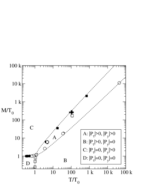
Figure 4: The 4d phase diagram in physical units. Filled symbols are for $N_{y}=2$, open ones for $N_{y}=4$. That they agree within errorbars indicates the absence of significant finite lattice spacing effects. The dashed curves represent the finite size scaling ansatz shown in Fig. 3, as well as its mirror with respect to the interchange $\tau\leftrightarrow y$.

The result of this procedure is shown in Fig. 4. This figure can directly be compared with Fig. 2 of [18]; we find perfect qualitative agreement. It may also be noted how remarkably well the finite size scaling ansatz in Eq. (3.1) can be used to parameterise a fit through the data points.

In principle it would also be interesting to check the parametric form proposed for the continuum critical curve (between, say, the regions A,B), $T\sim M/g^{2}\sim M\ln M$. We have however only a few data points, with modest resolution and without a precise extrapolation to the infinite volume and continuum limits, so we do not attempt that here.

4 Lattice results in five dimensions

We then move to 5d. Considerably less can be achieved now, since the theory is not renormalisable and thus a continuum limit cannot be systematically approached. Nevertheless, there are a number of issues which remain the same as in 4d: the 1-loop finite temperature effective potential for the phase of $P_{y}$ is still finite and shows symmetry breaking at zero temperature and small coupling [10], but no sign of symmetry restoration at high temperatures [18]. At the same time, non-perturbative arguments can again be presented according to which restoration should take place. We shall here study the issue in lattice theories defined with fixed finite lattice spacings.

$N_{\tau}$	$N_{y}$	$N_{1}\times N_{2}\times N_{3}$
1,2,4,6,8,12	1	$12^{3}$
1,2,4,8,12	2	$[8^{3}],12^{3},[14^{3},16^{3},18^{3}]$
1,2,4,8	4	$8^{3},12^{3},[14^{3}]$

Table 2: The volumes studied in the 5d case. Note that on account of the symmetry $N_{\tau}\leftrightarrow N_{y},P_{\tau}\leftrightarrow P_{y}$, some of them are effectively listed twice. The volumes in brackets have only been used for some of the values of $N_{\tau}$ shown.

The volumes used are listed in Table 2. The action, observables, and simulation techniques follow closely those in 4d, as described in Sec. 3.

4.1 Evidence for phase transitions

  

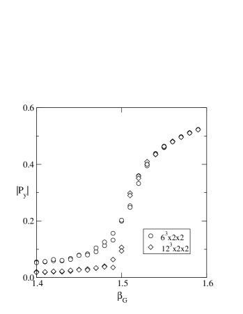
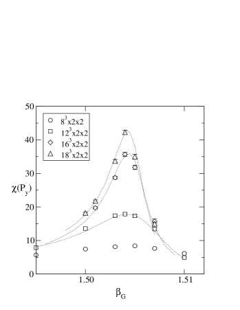
Figure 5: Examples of the absolute value of the Polyakov loop, $|P_{y}|$ (left), and the corresponding susceptibility, $\chi(P_{y})$ (right), as a function of $\beta_{G}$. The absence of significant hysteresis on the left indicates a second order phase transition. Note that $|P_{y}|\to 0$ for $\beta_{G}$ to the left of the susceptibility maximum, as the volume is increased. The points on the right have been joined together by reweighting.

  

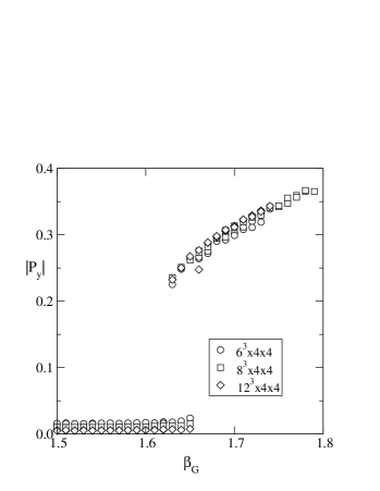
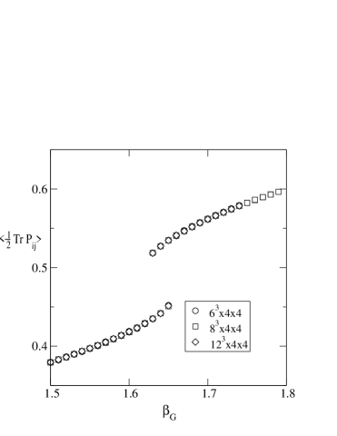
Figure 6: Examples of the absolute value of the Polyakov loop, $|P_{y}|$ (left), and the plaquette expectation value, $\langle{1\over 2}{\rm Tr\,}P_{ij}\rangle$ (right). The different branches show some metastability, or hysteresis, indicating a first order phase transition. Note again that $|P_{y}|\to 0$ for $\beta_{G}$ to the left of the transition point, as the volume is increased.

Typical signals for phase transitions in 5d are shown in Figs. 5, 6. In contrast to 4d, we now observe both second (Fig. 5) and first (Fig. 6) order phase transitions. The first order transition is also visible in the plaquette expectation value, as shown in Fig. 6 (right). Qualitatively, the possibility of an emergence of a first order signal may perhaps be understood via the universality arguments presented in Sec. 2.2.

4.2 Phase diagrams for fixed $N_{y}$

      

   

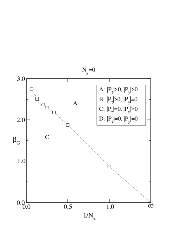
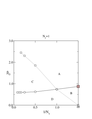
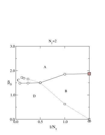
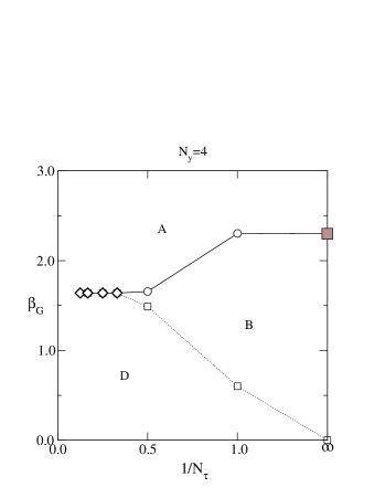
Figure 7: Phase diagrams for various $N_{y}$, in the 5d case. The lines connecting the simulation points are there to guide the eye only. The values for $N_{y}=0$ (top left), as well as for $1/N_{\tau}=\infty$ (filled boxes), are from [25, 26]. Open circles and boxes denote second order transitions, open diamonds first order ones.

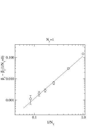
Figure 8: Finite-size scaling of the phase transition point determined from $\chi(P_{y})$ on volumes $12^{3}\times N_{\tau}\times 1$, as a function of $1/N_{\tau}$, together with a two-parameter fit according to Eq. (3.1) (fit for $\beta_{c}(N_{\tau}=\infty),c_{1}$, with a fixed $\nu=0.5$, $c_{2}=0.0$).

The results from different $N_{y}$ are summarised in Fig. 7. Again the existing data from the (3+1)d theory [25, 26] allow for a first check by comparing with a number of limiting values (filled boxes). We find good consistency.

A second check can be inferred from the scaling of $\beta_{c}$ close to $1/N_{\tau}=0$, as in Sec. 3.2. Now the universality class is that of the 4d Ising model, so that we expect a mean field exponent $\nu=0.5$ in Eq. (3.1), meaning a parabolic behaviour. In the 5d case our data is not precise enough to address the issue in great detail, but we do find that, say, the data with $N_{\tau}\mathop{\raise 1.29167pt\hbox{$>$\kern-7.5pt\raise-4.73611pt\hbox{$\sim$}}}N_{y}$ at $N_{y}=1$, can be fitted reasonably well with two free parameters, $\beta_{c}(N_{\tau}=\infty)$ and $c_{1}$ (Fig. 8).

4.3 Physical implications

Following Sec. 3.3, we can then draw the following physical conclusion from Fig. 7. Suppose we fix $\beta_{G}$, meaning that we fix the lattice spacing. Staying at this $\beta_{G}$ at zero temperature, $1/N_{\tau}=0$, let us increase $M$ until we are in the phase where the symmetry related to the phase of $P_{y}$ is broken, such that dimensional reduction to a 4d theory takes place (region C). This can be achieved by decreasing $N_{y}$, since $M=1/(aN_{y})$. Staying then on the horizontal line of a fixed $\beta_{G}$ and increasing the temperature by moving to the right in $1/N_{\tau}$ ($T=1/(aN_{\tau})$), we observe that at large enough values we may indeed cross the transition to the symmetric phase (region B). It is easy to see that if this happens by passing through the deconfined region A, then at the transition point $1/N_{\tau}>1/N_{y}$, implying $T_{c}>M$. Thus, the phase diagram is qualitatively as sketched in [18].

However, in contrast to the 4d case, the phenomenon described only takes place in a limited range of $N_{y}$, meaning that the continuum limit cannot be approached. Indeed, we find (Fig. 7, bottom right) that for $N_{y}=4$, the phase transition close to $1/N_{\tau}=0$ is of the first order [27], and the lines corresponding to the breaking of $P_{\tau},P_{y}$ have merged. This implies that there is no longer a low temperature phase (region C) which would be effectively four dimensional ($|P_{y}|>0$) and confining ($|P_{\tau}|=0$). We expect this to remain true also for $N_{y}>4$. Since the phase diagram changes qualitatively as $N_{y}$ is increased, one cannot define a meaningful line of constant physics, where discretisation artifacts would gradually vanish, as correlation lengths measured in lattice units grow.

We end with a brief comment on a related recent work, ref. [28]. The authors study a (4+1)-dimensional SU(2) gauge theory, corresponding to the axis $1/N_{\tau}=0$ in our figures, with asymmetric lattice spacings. As far as their data can be compared with ours, the results are consistent: with our symmetric lattice spacing, their study corresponds to $N_{y}\mathop{\raise 1.29167pt\hbox{$<$\kern-7.5pt\raise-4.73611pt\hbox{$\sim$}}}2$, implying indeed a second order phase transition. Our conclusion regarding the existence of a continuum limit in a genuine 5d theory is however different, for the reasons mentioned above. Of course a continuum limit does again exist for models of the type in [3], where the extra dimension is assumed inherently discretised (in other words, the continuum limit is only taken on the 4d planes, will the fifth dimension remains latticized), so that the lattice spacing is in a sense infinitely asymmetric.

5 Conclusions

We have discussed here the finite temperature behaviour of pure non-Abelian Yang-Mills theories, living in a space with a single circular extra dimension.

If the extra dimension is small enough, dimensional reduction takes place in asymptotically free (or weakly coupled) theories, as indicated by the standard perturbative analysis in terms of Kaluza-Klein excitations. At the same time, the circular dimension introduces a global Z($N$) symmetry in the system. If perturbation theory works, the symmetry must necessarily be broken, because the expectation value of the Polyakov loop in the extra direction is parametrically close to unity.

While just introduced through perturbative arguments, the same Z($N$) symmetry breaking can also be observed when the system is studied non-perturbatively. However, as we have demonstrated in this paper, this symmetry gets restored at high temperatures, $T_{c}>M$, where $M$ is the inverse of the perimeter of the extra dimension. This symmetry restoration is non-trivial because it is in contrast to straightforward perturbation theory.

Avoiding a domain wall problem in cosmology requires that such a symmetry restoration never takes place. We are thus lead to conclude that we would either have to change the model, or restrict the reheating temperature after inflation to be below $T_{c}$.

The simulations carried out to reach this conclusion were very simple. In fact, for $d=4$, the limiting cases of zero as well as infinite radii of the extra dimension could be extracted from the literature. We have here simply added a number of points in between, utilising small scale numerical simulations. However, we believe that our physical conclusions, as discussed above and summarised in Fig. 4, are new.

It is interesting to note that, at least on the resolution of a logarithmic scale, the phase diagram in Fig. 4 is well described by a finite size scaling ansatz in the whole range of interest. It is more difficult to determine the parametric behaviour of the continuum critical curves, but the symmetry restoration temperature is in any case typically above the inverse of the perimeter of the extra dimension, $T_{c}>M$.

There is less existing data available on the $d=5$ case. The new points we have added come again from small scale simulations. On a coarse lattice, the phase diagram remains qualitatively the same as at $d=4$. However, the continuum limit cannot be approached: on a finer lattice, some of the phase transitions turn into first order ones, and the physically relevant confining phase disappears. This means that one cannot define a “line of constant physics” along which to approach the continuum. Moreover, unlike in 4d, the correlation lengths do not diverge in lattice units as $N_{y}\to\infty$, if the first order signal continues to strengthen as expected. While the absence of a continuum limit is well known, we may have elaborated on it in a somewhat new way.

For cosmological applications, it is important to discuss the robustness of the phase diagram with respect to small modifications of the model. Let us reiterate that the main point of our study is that if a Z($N$) symmetry exists in the system and is spontaneously broken at zero temperature, then it does get restored at high temperatures, contrary to the prediction of straightforward perturbation theory. We would expect the main model dependence, then, to concern the zero temperature starting point, rather than actual finite temperature physics.

It is certainly true that it is possible to break the Z($N$) symmetry explicitly with a relatively small modification of the model. While matter fields in the adjoint representation do not break it, matter fields in the fundamental representation coupling to the covariant derivative $D_{y}$, do break the symmetry explicitly. Another generic way may be to change the topology of the spacetime, for instance by orbifolding, whereby the zero mode of the gauge field component $A_{y}$ vanishes, $A_{y}\equiv-A_{y}=0$ and thus $P_{y}=1$, or by considering more than one extra dimension of a specific structure. At the same time, other topological defects could of course potentially be introduced in such more complicated settings (see, e.g., [8, 29]). To summarise, the existence of domain walls at zero temperature is by no means generic, but requires a case by case study.

If the Z($N$) symmetry is indeed explicitly broken by some of the mechanisms mentioned, then cosmological constraints are much weaker [13]. Still, the existence of possibly relatively long-lived metastable Z($N$) vacua could lead to interesting phenomena, in analogy with the discussion in [30].

Let us end by recalling that there are other cosmological constraints similar to the one we have discussed. In particular, the overproduction of gravitons (or more generally very weakly coupled Kaluza-Klein excitations) at temperatures above the inverse radius, in case such particles propagate in the bulk, requires again a low reheating temperature, $T\mathop{\raise 1.29167pt\hbox{$<$\kern-7.5pt\raise-4.73611pt\hbox{$\sim$}}}M$ [31].

References

- [1] I. Antoniadis, Phys. Lett. B 246 (1990) 377.
- [2] K.R. Dienes, E. Dudas and T. Gherghetta, Nucl. Phys. B 537 (1999) 47 [hep-ph/9806292]; Proceedings of PASCOS’98, Boston, pp. 613-620 [hep-ph/9807522].
- [3] N. Arkani-Hamed, A.G. Cohen and H. Georgi, Phys. Rev. Lett. 86 (2001) 4757 [hep-th/0104005]; C.T. Hill, S. Pokorski and J. Wang, Phys. Rev. D 64 (2001) 105005 [hep-th/0104035].
- [4] G. ’t Hooft, Nucl. Phys. B 138 (1978) 1; Nucl. Phys. B 153 (1979) 141.
- [5] D.J. Gross, R.D. Pisarski and L.G. Yaffe, Rev. Mod. Phys. 53 (1981) 43.
- [6] N. Weiss, Phys. Rev. D 24 (1981) 475; Phys. Rev. D 25 (1982) 2667.
- [7] Y. Hosotani, Phys. Lett. B 126 (1983) 309.
- [8] K.M. Lee, R. Holman and E.W. Kolb, Phys. Rev. Lett. 59 (1987) 1069.
- [9] A. Nakamura, S. Hirenzaki and K. Shiraishi, Nucl. Phys. B 339 (1990) 533; A. Nakamura and K. Shiraishi, Prog. Theor. Phys. 84 (1990) 1100.
- [10] V.M. Belyaev and I.I. Kogan, Mod. Phys. Lett. A 7 (1992) 117.
- [11] T. Maki and K. Shiraishi, Nuovo Cim. A 107 (1994) 1219.
- [12] Y.B. Zeldovich, I.Y. Kobzarev and L.B. Okun, Zh. Eksp. Teor. Fiz. 67 (1974) 3 [Sov. Phys. JETP 40 (1974) 1].
- [13] A. Vilenkin and E.P.S. Shellard, Cosmic Strings and Other Topological Defects, Chapter 13 (Cambridge University Press, Cambridge, 1994).
- [14] S. Weinberg, Phys. Rev. D 9 (1974) 3357.
- [15] K. Jansen and M. Laine, Phys. Lett. B 435 (1998) 166 [hep-lat/9805024]; G. Bimonte, D. Iñiguez, A. Tarancón and C.L. Ullod, Nucl. Phys. B 559 (1999) 103 [hep-lat/9903027].
- [16] G.R. Dvali and G. Senjanović, Phys. Rev. Lett. 74 (1995) 5178 [hep-ph/9501387].
- [17] H. Casini and S. Sarkar, Phys. Rev. D 65 (2002) 025002 [hep-ph/0106272].
- [18] C.P. Korthals Altes and M. Laine, Phys. Lett. B 511 (2001) 269 [hep-ph/0104031].
- [19] B. Svetitsky and L.G. Yaffe, Nucl. Phys. B 210 (1982) 423.
- [20] J. Rudnick, Phys. Rev. B 18 (1978) 1406.
- [21] K. Kajantie, M. Laine, K. Rummukainen and M. Shaposhnikov, Nucl. Phys. B 503 (1997) 357 [hep-ph/9704416]; K. Kajantie, M. Laine, A. Rajantie, K. Rummukainen and M. Tsypin, JHEP 9811 (1998) 011 [hep-lat/9811004].
- [22] A.M. Ferrenberg and R.H. Swendsen, Phys. Rev. Lett. 61 (1988) 2635.
- [23] M. Teper, Phys. Lett. B 313 (1993) 417.
- [24] J. Engels, F. Karsch, E. Laermann, C. Legeland, M. Lütgemeier, B. Petersson and T. Scheideler, Nucl. Phys. B (Proc. Suppl.) 53 (1997) 420 [hep-lat/9608099].
- [25] R. Ben-Av, H.G. Evertz, M. Marcu and S. Solomon, Phys. Rev. D 44 (1991) 2953.
- [26] J. Fingberg, U. Heller and F. Karsch, Nucl. Phys. B 392 (1993) 493 [hep-lat/9208012].
- [27] M. Creutz, Phys. Rev. Lett. 43 (1979) 553; ibid. 43 (1979) 890 (E).
- [28] S. Ejiri, J. Kubo and M. Murata, Phys. Rev. D 62 (2000) 105025 [hep-ph/0006217]; S. Ejiri, S. Fujimoto and J. Kubo, Phys. Rev. D 66 (2002) 036002 [hep-lat/0204022].
- [29] G. Dvali, I.I. Kogan and M. Shifman, Phys. Rev. D 62 (2000) 106001 [hep-th/0006213].
- [30] J. Ignatius, K. Kajantie and K. Rummukainen, Phys. Rev. Lett. 68 (1992) 737.
- [31] K. Benakli and S. Davidson, Phys. Rev. D 60 (1999) 025004 [hep-ph/9810280].