Reshuffling the OPE:
Delocalized Operator Expansion

Abstract

A generalization of the operator product expansion for Euclidean correlators of gauge invariant QCD currents is presented. Each contribution to the modified expansion, which is based on a delocalized multipole expansion of a perturbatively determined coefficient function, sums up an infinite series of local operators. On a more formal level the delocalized operator expansion corresponds to an optimal choice of basis sets in the dual spaces which are associated with the interplay of perturbative and nonperturbative $N$-point correlations in a distorted vacuum. A consequence of the delocalized expansion is the running of condensates with the external momentum. Phenomenological evidence is gathered that the gluon condensate, often being the leading nonperturbative parameter in the OPE, is indeed a function of resolution. Within a model calculation of the nonperturbative corrections to the ground state energy of a heavy quarkonium system it is shown exemplarily that the convergence properties are better than those of the OPE. Potential applications of the delocalized operator expansion in view of estimates of the violation of local quark-hadron duality are discussed.

1 Introduction

1.1 Some historical remarks

Once again: Happy Birthday, Arkady! This is a very lively conference that I am happy to attend.

In this talk I would like to report about work done jointly with André Hoang. The subject is to formulate a framework for a generalization of Wilson’s operator product expansion (OPE), to confront this framework with experiment, and to demonstrate its usefulness in some model calculations.

As a warm-up I remind you of some of the OPE applications. The OPE is a powerful tool for the treatment of conformally invariant field theories where its convergence is explicitly shown. Unfortunately, this feature does not survive in realistic, four-dimensional field theories. Here the expansion is believed to be asymptotic at best.

The construction of effective theories like HQET or of the effective Hamiltonians of electroweak theory are crucially relying on the OPE which determines effective vertices by a perturbative matching of amplitudes with those of the fundamental theory. Heavy fields are effectively integrated out in this procedure (see [ [1]] and references therein).

The OPE turned out to be important for a semi-perturbative derivation of the exact $\beta$ function in $N=1$ super Yang-Mills theory [ [2]].

And, finally, there is a major application in QCD sum rules [ [3]] where the “theoretical side” of a dispersion relation for the correlator of gauge invariant currents is represented in terms of an OPE. The occurence of power corrections to the low-order in $\alpha_{s}$ perturbative result can be argued from the summation of bubble graphs inducing so-called infrared renormalons, and formal contact to the OPE can be made [ [4]]. A practical version of the OPE was proposed by Shifman, Vainshtein, and Zakharov in [ [3]] where nonperturbative factors in the power corrections, the QCD condensates, are viewed as universal parameters of the QCD vacuum to be determined by experiment. Due to the universality of the condensates this method is rather predictive in practice.

1.2 Problems of the OPE in QCD

Despite its many successes in the framework of the QCD sum rule method there are some unanswered questions concerning the convergence properties of the OPE. Answering these questions very likely resolves the problems connected with local quark-hadron duality (see [ [5]] in references therein) which can be formulated as follows.

Given analyticity of the correlator away from the positive real axis and invoking the optical theorem the discontinuity of the correlator at time-like momenta should yield the spectral function of the hadronic channel which corresponds to the QCD current in the correlator. This procedure, however, fails badly if a “practical” OPE with a small number of power corrections is used. Whereas the experimentally measured spectral function shows resonance wiggles at moderate time-like momenta a continuation of the OPE generates a smooth behavior down to small momenta. This may not harm the sum rule method since the relevant quantity there is a spectral integral, that is, an average over resonances which agrees quite well with the average over the associated discontinuity of the OPE. However, in applications, where the local properties of OPE discontinuities are needed [ [6]], the violation of local quark-hadron duality can induce large errors.

Another concern, which is connected with the violation of local quark-hadron duality, is the asymptotic nature of the expansion. Asymptotic behavior can be argued from estimates of operator averages using the instanton gas approximation [ [3]] or by appealing to the renormalon idea. From the OPE itself, where naively an expansion in powers of $\Lambda_{QCD}/Q$ is assumed, there is no way of estimating the critical dimension at which the expansion ceases to approximate. In the framework of a delocalized expansion it was argued in [ [7]] that the knowledge about nonperturbative, gauge invariant correlation functions would allow for such an estimate if the decay of effective correlation length with mass dimension is sufficiently fast.

The central theme of this talk is a nonlocal generalization of the OPE which has the potential to cure the above short-comings.

2 Delocalized operator expansion

The OPE of the correlator of a current $j$ reads

$$i\int d^{4}x\,\mbox{e}^{iqx}\left\langle Tj(x)j(0)\right\rangle=Q^{2}\sum_{d=0}\sum_{l=1}^{l_{d}}c_{dl}(Q^{2})\left\langle O_{dl}(0)\right\rangle\,,\ \ (Q^{2}=-q^{2}>0)\,,$$

where $d,l$ run over the dimension and the field content of the local operator $O_{dl}$, respectively. The Wilson coefficient $c_{dl}$ is perturbatively calculable. The expansion (2) contains reducible chains of operators, such as

$$G^{2},GD^{2}G,GD^{4}G,GD^{6}G...\,,$$

$$\bar{q}q,\bar{q}D_{\mu}\gamma_{\mu}q,\bar{q}D^{2}q,\bar{q}D^{2}D_{\mu}\gamma_{\mu}q\,,$$ (2)

$D_{\mu}$ denotes the gauge covariant derivative. Here “reducible” refers to the fact that each chain can be obtained from a Taylor expansion of an associated gauge invariant 2-point correlator which is not decomposible into gauge invariant factors. Examples, which correspond to the chains in (2), are the gluonic field strength correlator [ [8]]

$$g_{\mu\nu\kappa\lambda}(x)\equiv tr\left\langle g^{2}G_{\mu\nu}(x)\,P\mbox{e}^{ig\int_{0}^{x}dz_{\mu}A_{\mu}(z)}\,G_{\kappa\lambda}(0)P\mbox{e}^{ig\int_{x}^{0}dz_{\mu}A_{\mu}(z)}\right\rangle$$ (3)

and the bilocal quark “condensate”

$$q(x)\equiv\left\langle\bar{q}(x)\,P\mbox{e}^{ig\int_{0}^{x}dz_{\mu}A_{\mu}(z)}\,q(0)\right\rangle\,,$$ (4)

where $P$ denotes path ordering. For lattice measurements the path connecting the points $0$ and $x$ is taken to be a straight line. This should capture the largest scale $\Lambda$ in the nonperturbative decay of the correlator. The general case of $N$-point correlations will be addressed below. The effect of a delocalized expansion is a partial summation of such a chain in each order of the momentum expansion of the perturbative coefficient. This leads to an improvement of the convergence properties.

Let me make this explicit for the case of 2-point correlations in a 1-dimensional Euclidean world [ [9]]. The contribution to the OPE, which arises from this, can formally be written as

$$\int_{-\infty}^{\infty}dx\,f(x)\,g(x) = \int dx\,dy\,f(y)\,\delta(x-y)\,g(x)$$ (5)

$$= \int dx\,dy\,f(y)\,\bigg{[}\,\sum_{n=0}^{\infty}\frac{(-1)^{n}}{n!}\,y^{n}\delta^{(n)}(x)\,\bigg{]}\,g(x)$$

$$= \sum_{n=0}^{\infty}\bigg{[}\,\int dy\,f(y)\,y^{n}\,\bigg{]}\,\left[\int dx\,\frac{(-1)^{n}}{n!}\delta^{(n)}(x)\,g(x)\right]$$

$$\equiv \sum_{n=0}^{\infty}f_{n}(\infty)\,g_{n}(\infty)\,.$$

Here $f(x)$ is associated with perturbative correlations whereas $g(x)$ describes nonlocal, nonperturbative effects. The integral expressions in the first and second square bracket correspond to local Wilson coefficients and operators of the like of (2), respectively. From (5) it is seen that the part of the OPE being generated by 2-point correlations is induced by a bilinear form $(\cdot\,,\cdot)\equiv\int dx\cdot\times\,\cdot$. The expansion (5) corresponds to a specific choice of basis $\{\tilde{e}_{n}(\infty),e_{n}(\infty)\}$ in the associated dual space of square integrable functions where

$$\tilde{e}_{n}(\infty)=y^{n}\ \ \ \ \ \ \mbox{and}\ \ \ \ \ e_{n}(\infty)=\frac{(-1)^{n}}{n!}\,\delta^{(n)}(x)\,.$$ (6)

and we have orthonormality

$$\left(\,e_{n}\,,\,\tilde{e}_{m}\,\right)\,=\,\delta_{nm}\,.$$ (7)

From Eq. (5) it follows that

$$f(x) = \sum_{n=0}^{\infty}\,\bigg{[}\,\int dy\,f(y)\,y^{n}\,\bigg{]}\,\frac{(-1)^{n}}{n!}\,\delta^{(n)}(x)\,.$$ (8)

This corresponds to an expansion of the perturbative factor $f(x)$ into degenerate, that is, zero-width multipoles.

Figure 1: Schematic drawing of the short-distance function $f(x)$ and the nonperturbative 2-point-correlator $g(x)$ illustrating the scale hierarchy $\Delta_{f}/\Delta_{g}\sim\Lambda/Q\ll 1$.

It is suggestive that an expansion into multipoles of width $\sim\Omega^{-1}$, which is comparable with $\Delta_{f}\sim Q^{-1}$, converges better (see Fig. 1). Like the OPE this expansion is controlled by powers of $\frac{\Delta_{f}}{\Delta_{g}}\sim\frac{\Lambda}{Q}$, and it breaks down if $\Delta_{f}\sim Delta_{g}$. The expansion into finite-width multipoles corresponds to a change of basis in dual space. Rather than expanding into the basis $\{\tilde{e}_{n}(\infty),e_{n}(\infty)\}$ one may expand into $\{\tilde{e}_{n}(\Omega),e_{n}(\Omega)\}$ where

$$\tilde{e}_{n}^{\Omega}(x)=\frac{H_{n}(\Omega x)}{(2\,\Omega)^{n}}\,,\ \ \ e_{n}^{\Omega}(x)\equiv\frac{\Omega^{n+1}}{\sqrt{\pi}\,n!}\,H_{n}(\Omega x)\,\mbox{e}^{-\Omega^{2}x^{2}}$$ (9)

We then have

$$\int dx\,f(x)\,g(x)=\sum_{n=0}^{\infty}f_{n}(\Omega)\,g_{n}(\Omega)\,.$$ (10)

In (9) $H_{n}$ denotes the $n$th Hermite polynomial. An expansion into any other basis that allows for a sensible multipole expansion of $f(x)$ is possible, and the restriction to a Gaussian based expansion is just for definiteness. Note that (9) reduces to (6) in the limit $\Omega\to\infty$. According to (9) the transformations, which link a basis with resolution parameter $\Omega$ to a basis with $\Omega^{\prime}$, form a 1-parameter group. The moments $f_{n}(\Omega)$ in (10) have finite expansions into the Wilson coefficients $f_{n}(\infty)$

$$f_{0}(\Omega)=f_{0}(\infty)\,,\ f_{2}(\Omega)=f_{2}(\infty)-\frac{1}{2\Omega^{2}}f_{0}(\infty)\,,\cdots\,.$$ (11)

Chosing a particular basis and a value for $\Omega$ is analogous to a choice of regularization and normalization point in pure perturbation theory. In practice (11) enables to consider perturbative renormalization and delocalized operator expansion (DOE) separately. The expansion of $g(\Omega)$ into local condensates is infinite, for example

$$g_{0}(\Omega)=g_{0}(\infty)+\frac{1}{2\Omega^{2}}g_{2}(\infty)+\cdots\,.$$ (12)

To evaluate sums like in (12) one would have to know infinitely many anomalous dimensions and condensates. On the other hand, one may be more pragmatic and start with a (lattice inspired) model for $g(x)$ which is believed to contain the information about all $g_{n}(\infty)$. To each order $\frac{\Lambda}{\Omega}$ one may then derive evolution equations for $f_{n}(\Omega)$ and $g_{n}(\Omega)$ which sum these contributions to all orders [ [9]].

Setting $\Omega=Q$, the parametric organization of the expansion in $\frac{\Lambda}{Q}$ up to an overall factor is

$$f_{0}(Q)\times g_{0}(Q) \sim \left(\frac{\Lambda}{Q}\right)^{0}\times\{\left(\frac{\Lambda}{Q}\right)^{0}+\left(\frac{\Lambda}{Q}\right)^{2}+\cdots\}$$

$$f_{2}(Q)\times g_{2}(Q) \sim \left(\frac{\Lambda}{Q}\right)^{2}\times\{\left(\frac{\Lambda}{Q}\right)^{0}+\left(\frac{\Lambda}{Q}\right)^{2}+\cdots\}$$ (13)

$$\vdots \ \ \ \ \ \ \ \ \ \ \ \ \ \ \ \ \ .$$

The generalization to $K$-dimensional Euclidean space is straightforward [ [9]]. It also allows for a treatment of $N$-point correlations in 4-dimensional space. In particular, the $n=0$ term of the contribution to the DOE from 2-gluon correlations yields the local Wilson coefficient times a “runnning gluon condensate” ($Q=\Omega$).

3 Applications

3.1 Gluonic field strength correlator

To have a well-motivated model for $g(x)$ for the case of 2-gluon correlations we appeal to a parametrization of the gluonic field strength correlator (3) as it was proposed in [ [8]]

$$g_{\mu\nu\kappa\lambda}(x) \equiv (\delta_{\mu\kappa}\delta_{\nu\lambda}-\delta_{\mu\lambda}\delta_{\nu\kappa})[D(x^{2})+D_{1}(x^{2})]+$$ (14)

$$(x_{\mu}x_{\kappa}\delta_{\nu\lambda}-x_{\mu}x_{\lambda}\delta_{\nu\kappa}+x_{\nu}x_{\lambda}\delta_{\mu\kappa}-x_{\nu}x_{\kappa}\delta_{\mu\lambda})\frac{\partial D_{1}(x^{2})}{\partial x^{2}}\,.$$

In a lattice measurement [ [10]] the scalar functions $D$ and $D_{1}$ were parametrized as

$$D(x^{2}) = A_{0}\exp[-|x|/\lambda_{A}]+\frac{a_{0}}{|x|^{4}}\exp[-|x|/\lambda_{a}]\,,$$

$$D_{1}(x^{2}) = A_{1}\exp[-|x|/\lambda_{A}]+\frac{a_{1}}{|x|^{4}}\exp[-|x|/\lambda_{a}]\,,$$ (15)

where the purely exponentially decaying terms are attributed to purely nonperturbative dynamics. The measurements at various quark masses for dynamical light quarks indicate that for $|x|\leq\lambda_{A}$ the nonperturbative contribution to $D$ dominates the nonperturbative contribution to $D_{1}$ implying that the tensor structure of $g_{\mu\nu\kappa\lambda}$ is identical to that of the corresponding local operator obtained by letting $x\to 0$. This feature leads to great simplifications.

3.2 Extraction of the running gluon condensate

Using the DOE instead of the OPE, the running gluon condensate can be extracted from experiment in channels where 2-gluon correlations are dominant. We have done this for the $V+A$ correlator and the charmonium system. For a more detailed presentation see [ [9]].

3.2.1 Sum rules for the V+A correlator

The spectral function for light quark production in the $V+A$ channel has been remeasured recently from hadronic $\tau$ decays for $q^{2}\leq m_{\tau}^{2}$ by Aleph [ [11]] and Opal [ [12]]. In the OPE the associated current correlator is dominated by the gluon condensate, and the dimension $6$ power corrections that are not due to a double covariant derivative in the local gluon condensate are suppressed. The corresponding currents are $j_{\mu}^{L/R}=\bar{u}\gamma_{\mu}(1\pm\gamma_{5})d$ and the relevant correlator in the chiral limit reads

$$i\int d^{4}\!x\,\mbox{e}^{iqx}\left\langle Tj_{\mu}^{L}(x)j_{\nu}^{R}(0)\right\rangle\, = \,(q_{\mu}q_{\nu}-q^{2}g_{\mu\nu})\,\Pi^{\rm V+A}(Q^{2})\,,\qquad Q^{2}=-q^{2}\,.$$

Since the correlator $\Pi(Q^{2})^{\rm V+A}$ is cutoff-dependent itself, we investigate the Adler function

$$D(Q^{2})\,\equiv\,-Q^{2}\,\frac{\partial\,\Pi^{\rm V+A}(Q^{2})}{\partial\,Q^{2}}\,=\,\frac{Q^{2}}{\pi}\,\int_{0}^{\infty}ds\,\frac{\mbox{Im}\,\Pi^{\rm V+A}(s)}{(s+Q^{2})^{2}}\,.$$ (17)

For the corresponding experimental V+A spectral function we have used the Aleph measurement in the resonance region up to $2.2$ GeV². For the continuum region above $2.2$ GeV² we used 3-loop perturbation theory for $\alpha_{s}(M_{Z})=0.118$, and we have set the renormalization scale $\mu$ to $Q$. We remark that the pion pole of the axial vector contribution has to be taken into account in order to yield a consistent description in terms of the OPE for asymptotically large $Q$ [ [13]]. We have checked that the known perturbative contributions to the Adler function show good convergence properties. For $Q$ between $1.0$ and $2.0$ GeV and setting $\mu=Q$, the 3-loop (two-loop) corrections amount to $5\%$ ($7\%$) and $0.5\%$ ($1.4\%$), respectively. On the other hand, the O$(\alpha_{s})$ correction to the Wilson coefficient of the gluon condensate are between $-16\%$ and $-6\%$ for $\mu$ between $0.8$ and $2.0$ GeV. We have compared the local dimension $6$ contributions contained in the running gluon condensate with the sum of all dimension $6$ terms in the OPE as they were determined in [ [13]]. We again found that the corresponding dimension $6$ contributions have equal sign and roughly the same size.

Our result for the running gluon condensate as a function of $Q$ is shown in Fig. 2.

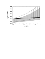
Figure 2: The running gluon condensate as a function of $Q$ when extracted from the Adler function. The grey area represents the allowed region using perturbation theory at O$(\alpha_{s}^{3})$ and the striped region using perturbation theory at O$(\alpha_{s}^{2})$. The thick solid line denotes the running gluon condensate ($\Omega=Q$) from the lattice-inspired ansatz.

for $1$ GeV$\leq Q\leq 2$ GeV. The uncertainties are due to the experimental errors in the spectral function and a variation of the renormalization scale $\mu$ in the range $Q\pm 0.25$ GeV. The strong coupling has been fixed at $\alpha_{s}(M_{Z})=0.118$. We have restricted our analysis to the range $1\,\,\mbox{GeV}<Q<2\,\,\mbox{GeV}$ because for $Q\mathrel{\raise 1.29167pt\hbox{$<$\kern-7.5pt\lower 4.30554pt\hbox{$\sim$}}}1$ GeV perturbation theory becomes unreliable and for $Q\mathrel{\raise 1.29167pt\hbox{$>$\kern-7.5pt\lower 4.30554pt\hbox{$\sim$}}}2$ GeV the experimentally unknown part of the spectral function at $s\geq 2.2$ GeV² is being probed. The thick black line in Fig. 2 shows the running gluon condensate obtained from the lattice-inspired model of the last section for $\Omega=Q$. We find that our result for the running gluon condensate as a function of $Q$ is consistent with a function that increases with $Q$.

3.2.2 Charmonium sum rules

The determination of the local gluon condensate $\Big{\langle}\frac{\alpha_{s}}{\pi}\,G^{2}\Big{\rangle}(\infty)$ from charmonium sum rules was pioneered in Refs. [ [15]]. By now there is a vast literature on computations of Wilson coefficients to various loop-orders and various dimensions of the power corrections in the correlator of two heavy quark currents including updated analyses of the corresponding sum rules (see e.g. Refs. [ [16, 17]]).

The relevant correlator is

$$(q_{\mu}q_{\nu}-q^{2}\,g_{\mu\nu})\,\Pi^{c}(Q^{2})\,=\,i\int d^{4}x\,\mbox{e}^{iqx}\left\langle Tj^{c}_{\mu}(x)j^{c}_{\nu}(0)\right\rangle\,,\qquad Q^{2}=-q^{2}\,,$$ (18)

where $j_{\mu}\equiv\bar{c}\gamma_{\mu}c$, and the $n$-th moment is defined as

$$M_{n}\,=\,\frac{1}{n!}\,\left.\Big{(}\!-\frac{d}{dQ^{2}}\Big{)}^{n}\,\Pi^{c}(Q^{2})\,\right|_{Q^{2}=0}\,.$$ (19)

Assuming analyticity of $\Pi^{c}$ in $Q^{2}$ away from the negative, real axis and employing the optical theorem, the $n$th moment can be expressed as a dispersion integral over the charm pair cross section in $e^{+}e^{-}$ annihilation,

$$M_{n}\,=\,\frac{1}{12\pi^{2}\,Q_{c}^{2}}\,\int\frac{ds}{s^{n+1}}\,\frac{\sigma_{e^{+}e^{-}\to c\bar{c}+X}(s)}{\sigma_{e^{+}e^{-}\to\mu^{+}\mu^{-}}(s)}\,,$$ (20)

where $s$ is the square of the c.m. energy and $Q_{c}=2/3$. We consider the ratio [ [15]]

$$r_{n}\,\equiv\,\frac{M_{n}}{M_{n-1}}$$ (21)

and extract the running gluon condensate as a function of $n$ from the equality of the theoretical ratio using Eq. (19) and the ratio based on Eq. (20) determined from experimental data.

For the experimental moments we use the compilation presented in Ref. [ [18]], where the spectral function is split into contributions from the charmonium resonances, the charm threshold region, and the continuum. For the latter the authors of Ref. [ [18]] used perturbation theory since no experimental data are available for the continuum region. We have assigned a 10% error for the spectral function in the continuum region. For the purely perturbative contribution of the theoretical moments we used the compilation of analytic O$(\alpha_{s}^{2})$ results from Ref. [ [18]] and adopted the $\overline{\mbox{MS}}$ mass definition $\overline{m}_{c}(\overline{m}_{c})$ (for any renormalization scale $\mu$). We have used the one-loop expression for the Wilson coefficient of the gluon condensate, and we have checked that for $n\leq 8$ the perturbative O$(\alpha_{s}^{2})$ corrections do not exceed 50% of the O$(\alpha_{s})$ corrections for $\mu$ between $1$ and $4$ GeV.

Our result for the running gluon condensate as a function of $n$ is shown in Fig. 3. For each value of $\overline{m}_{c}(\overline{m}_{c})$ and $n$ the area between the upper and lower symbols represents the uncertainty due to the experimental errors of the moments and variations of $\alpha_{s}(M_{Z})$ between $0.116$ and $0.120$ and of $\mu$ between $1$ and $3$ GeV.

Figure 3: The running gluon condensate as a function of $n$ when extracted from the ratio of moments $r_{n}$ for $\overline{m}_{c}(\overline{m}_{c})=1.23$ (white triangles), $1.24$ (black stars), $1.25$ (white squares) and $1.26$ GeV (black triangles). The area between the upper and lower symbols represent the uncertainties. The thick solid line indicates the running gluon condensate as it is obtained from the lattice-inspired model for $g(x)$.)

We see that the running gluon condensate appears to be a decreasing function of $n$. Since the exact width of the short-distance function $f$ for the moments is unknown we estimate it using physical arguments. For large $n$, i.e.  in the nonrelativistic regime, the width is of the order of the quark c.m. kinetic energy $mv^{2}$, which scales like $m/n$ because the average quark velocity in the $n$-th moment scales like $1/\sqrt{n}$. [ [19]] For small $n$ the relevant short-distance scale is just the quark mass. Therefore, we take $\Omega=2m_{c}/n$ as the most appropriate choice of the resolution scale. In Fig. 3 the running gluon condensate is displayed for $\lambda_{A}^{-1}=0.7$ GeV and, exemplarily, $A_{0}=0.04$ (i.e. $\langle(\alpha_{s}/\pi)G^{2}\rangle_{\rm lat}(\infty)=0.024\,\,\mbox{GeV}^{4}$) and for $\Omega=(2.5\,\,\mbox{GeV})/n$ as the thick solid line. We find that the $n$-dependence of the lattice inspired running gluon condensate and our fit result from the charmonium sum rules are consistent. However, the uncertainties of our extraction are still quite large, particularly for $n=2$, where the sensitivity to the error in the continuum region is enhanced. We also note that the values for the running gluon condensate tend to decrease with increasing charm quark mass. For $\overline{m}_{c}(\overline{m}_{c})=1.27$ GeV we find that $\langle(\alpha_{s}/\pi)G^{2}\rangle$ ranges from $-0.01\,\,\mbox{GeV}^{4}$ to $+0.01\,\,\mbox{GeV}^{4}$ and shifts further towards negative values for $\overline{m}_{c}(\overline{m}_{c})\mathrel{\raise 1.29167pt\hbox{$>$\kern-7.5pt\lower 4.30554pt\hbox{$\sim$}}}1.28$ GeV for all $n>2$. Assuming the reliability of the DOE as well as the local OPE in describing the nonperturbative effects in the charmonium sum rules and that the Euclidean scalar functions $D(x)$ and $D_{1}(x)$ in the parametrization (14) are positive definite, our result disfavors $\overline{m}_{c}(\overline{m}_{c})\mathrel{\raise 1.29167pt\hbox{$>$\kern-7.5pt\lower 4.30554pt\hbox{$\sim$}}}1.28$ GeV.

3.3 A model calculation

Among the early applications of the OPE in QCD was the analysis of nonperturbative effects in heavy quarkonium systems [ [20, 21, 22]]. Heavy quarkonium systems are nonrelativistic quark-antiquark bound states for which there is the following hierarchy of the relevant physical scales $m$ (heavy quark mass), $mv$ (relative momentum), $mv^{2}$ (kinetic energy) and $\Lambda_{\rm QCD}$:

$$m\,\gg\,mv\,\gg\,mv^{2}\,\gg\,\Lambda_{\rm QCD}\,.$$ (22)

Thus the spatial size of the quarkonium system $\sim(mv)^{-1}$ is much smaller than the typical dynamical time scale $\sim(mv^{2})^{-1}$ effectively rendering the problem 1-dimensional. In this section we demonstrate the DOE for the nonperturbative corrections to the $n^{\,2s+1}L_{j}=1^{\,3}S_{1}$ ground state. We adopt the local version of the multipole expansion (OPE) for the expansion in the ratios of the scales $m$, $mv$ and $mv^{2}$. The resolution dependent expansion (DOE) is applied with respect to the ratio of the scales $mv^{2}$ and $\Lambda_{\rm QCD}$. The former expansion amounts to the usual treatment of the dominant perturbative dynamics by means of a nonrelativistic two-body Schrödinger equation. The interaction with the nonperturbative vacuum is accounted for by two insertions of the local $\mathbf{x}\mathbf{E}$ dipole operator, $\mathbf{E}$ being the chromoelectric field [ [20]]. The chain of VEV’s of the two gluon operator with increasing numbers of covariant derivatives times powers of quark-antiquark octet propagators [ [20]], i.e. the expansion in $\Lambda/mv^{2}$, is treated using the DOE.

At leading order in the local multipole expansion with respect to the scales $m$, $mv$, and $mv^{2}$ the expression for the nonperturbative corrections to the ground state energy reads

$$E^{np}\,=\,\int_{-\infty}^{\infty}\!dt\,f(t)\,g(t)\,,$$ (23)

where

$$f(t)\, = \,\frac{1}{36}\,\int\frac{dq_{0}}{2\pi}\,\mbox{e}^{iq_{0}(it)}\,\int\!d^{3}\mathbf{x}\int\!d^{3}\mathbf{y}\,\phi(x)\,(\mathbf{x}\mathbf{y})\,G_{O}\bigg{(}\mathbf{x},\mathbf{y},-\frac{k^{2}}{m}-q_{0}\bigg{)}\,\phi(y)\,,$$

with

$$G_{O}\bigg{(}\mathbf{x},\mathbf{y},-\frac{k^{2}}{m}\bigg{)} = \sum_{l=0}^{\infty}\,(2l+1)\,P_{l}\bigg{(}\frac{\mathbf{x}\mathbf{y}}{xy}\bigg{)}\,G_{l}\bigg{(}x,y,-\frac{k^{2}}{m}\bigg{)}\,,$$

$$G_{l}\bigg{(}x,y,-\frac{k^{2}}{m}\bigg{)} = \frac{mk}{2\pi}\,(2kx)^{l}\,(2ky)^{l}\,\mbox{e}^{-k(x+y)}\,$$

$$\sum_{s=0}^{\infty}\,\frac{L_{s}^{2l+1}(2kx)\,L_{s}^{2l+1}(2ky)\,s!}{(s+l+1-\frac{m\,\alpha_{s}}{12\,k})\,(s+2l+1)!}\,,$$

$$\phi(x) = \frac{k^{3/2}}{\sqrt{\pi}}\,\mbox{e}^{-kx}\,,\ \ \ \ k=\frac{2}{3}\,m\alpha_{s}\,.$$ (25)

The term $G_{O}$ is the quark-antiquark octet Green-function [ [22]], and $\phi$ denotes the ground state wave function. The functions $P_{n}$ and $L_{n}^{k}$ are the Legendre and Laguerre polynomials, respectively. We note that $t$ is the Euclidean time. This is the origin of the term $it$ in the exponent appearing in the definition of the function $f$.

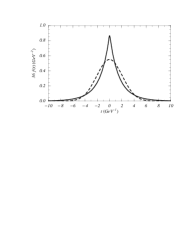
Figure 4: The perturbative short-distance function $f(t)$ for $m=5$ GeV and $\alpha_{s}=0.39$ (solid line) and the leading term in the delocalized multipole expansion of $f(t)$ for $\Omega=k^{2}/m$ (dashed line).

In Fig. 4 the function $f(t)$ (solid line) is displayed for $m=5$ GeV and $\alpha_{s}=0.39$. Since the spatial extension of the quarkonium system is neglected and the average time between interactions with the vacuum is of the order of the inverse kinetic energy, the characteristic width of $f$ is of order $(mv^{2})^{-1}\sim(m\alpha_{s}^{2})^{-1}$. As a comparison we have also displayed the function $[\int dt^{\prime}f(t^{\prime})\tilde{e}_{0}^{\Omega}(t^{\prime})]e_{0}^{\Omega}(t)$ for $\Omega=k^{2}/m$ (dashed line), which is the leading term in the delocalized multipole expansion of $f$. The values of the first few local multipole moments $f_{n}(\infty)$, which correspond to the local Wilson coefficients, read

$$\begin{array}[]{ll}f_{0}(\infty)\,=\,1.6518\,\frac{m}{36\,k^{4}}\,,&f_{2}(\infty)\,=\,1.3130\,\frac{m^{3}}{36\,k^{8}}\,,\\[8.53581pt] f_{4}(\infty)\,=\,7.7570\,\frac{m^{5}}{36\,k^{12}}\,,&f_{6}(\infty)\,=\,30.492\,\frac{m^{7}}{36\,k^{16}}\,,\\[8.53581pt] f_{8}(\infty)\,=\,4474.1\,\frac{m^{9}}{36\,k^{20}}\,,&f_{10}(\infty)\,=\,262709.3\,\frac{m^{11}}{36\,k^{24}}\,,\ldots\,.\end{array}$$ (26)

The term $f_{0}(\infty)$ agrees with Ref. [ [21, 22]] and $f_{2}(\infty)$ with Ref. [ [14]]. The results for $f_{n>2}(\infty)$ are new.

Let us compare the local expansion of $E^{np}$ with the resolution-dependent expansion using the basis functions of Eq. (9). For the nonperturbative gluonic field strength correlator we use a lattice inspired model of the form

$$g(t) = 12\,A_{0}\,\exp\Big{(}-\sqrt{t^{2}+\lambda_{A}^{2}}/\lambda_{A}+1\Big{)}\,,$$

$$A_{0} = 0.04~{}\mbox{GeV}^{4}\,,\qquad\lambda_{A}^{-1}\,=\,0.7~{}\mbox{GeV}\,,$$ (27)

This model has an exponential large-time behavior and a smooth behavior for small $t$. The local dimension $4$ gluon condensate in this model is

$$\Big{\langle}\frac{\alpha_{s}}{\pi}\,G_{\mu\nu}^{a}G_{\mu\nu}^{a}\Big{\rangle}\,=\,\frac{6\,A_{0}}{\pi^{2}}\,=\,0.024\,\,\mbox{GeV}^{4}\,.$$ (28)

In Tab. 3.3 we have displayed the exact result and the first four terms of the resolution-dependent expansion of $E^{np}$ for the quark masses $m=5,25,45,90,175$ GeV and for $\Omega=\infty$ and $\Omega=k^{2}/m$. For each value of the quark mass the strong coupling has been fixed by the relation $\alpha_{s}=\alpha_{s}(k)$.

Nonperturbative corrections to the heavy quarkonium ground state level at leading order in the multipole expansion with respect to the scales $m$, $mv$ and $mv^{2}$ for various quark masses $m$ based on the model in Eq. (27). Displayed are the exact result and the first few orders in the DOE for $\Omega=\infty$ and $\Omega=k^{2}/m$. The numbers are rounded off to units of $0.1$, $0.01$ or $0.001$ MeV. $\Omega=\infty$ $\Omega=k^{2}/m$ $m$ $k^{2}/m$ $E^{np}$ $f_{n}g_{n}$ $\sum^{n}_{i=0}f_{i}g_{i}$ $f_{n}g_{n}$ $\sum^{n}_{i=0}f_{i}g_{i}$ (GeV) $\alpha_{s}$ (MeV) (MeV) $n$ (MeV) (MeV) (MeV) (MeV) $5$ $0.39$ $0.338$ $24.8$ 0 $38.6$ $38.6$ $24.2$ $24.2$ 2 $-65.7$ $-27.2$ $-3.9$ $20.3$ 4 $832.7$ $805.5$ $12.1$ $32.4$ 6 $-35048.0$ $-34242.4$ $-43.1$ $-10.8$ $25$ $0.23$ $0.588$ $12.6$ 0 $16.0$ $16.0$ $12.8$ $12.8$ 2 $-9.0$ $7.0$ $-1.2$ $11.5$ 4 $37.8$ $44.8$ $2.6$ $14.1$ 6 $-526.6$ $-481.8$ $-6.7$ $7.4$ $45$ $0.19$ $0.722$ $4.9$ 0 $5.9$ $5.9$ $5.0$ $5.0$ 2 $-2.2$ $3.7$ $-0.4$ $4.6$ 4 $6.1$ $9.8$ $0.7$ $5.3$ 6 $-56.4$ $-46.6$ $-1.4$ $3.8$ $90$ $0.17$ $1.156$ $1.05$ 0 $1.15$ $1.15$ $1.07$ $1.07$ 2 $-0.17$ $0.98$ $-0.04$ $1.02$ 4 $0.18$ $1.16$ $0.04$ $1.07$ 6 $-0.65$ $0.51$ $-0.07$ $1.00$ $175$ $0.15$ $1.750$ $0.245$ 0 $0.258$ $0.258$ $0.249$ $0.249$ 2 $-0.016$ $0.242$ $-0.005$ $0.244$ 4 $0.008$ $0.250$ $0.003$ $0.247$ 6 $-0.012$ $0.237$ $-0.003$ $0.244$

Note that the series are all asymptotic, i.e.  there is no convergence for any resolution. The local expansion ($\Omega=\infty$) is quite badly behaved for smaller quark masses because for $k^{2}/m\mathrel{\raise 1.29167pt\hbox{$<$\kern-7.5pt\lower 4.30554pt\hbox{$\sim$}}}\lambda_{A}^{-1}$ any local expansion is meaningless. In particular, for $m=5$ GeV the subleading dimension $6$ term is already larger than the parametrically leading dimension $4$ term. This is consistent with the size of the dimension $6$ term based on a phenomenological estimate of the local dimension $6$ condensate. For quark masses, where $k^{2}/m\mathrel{\raise 1.29167pt\hbox{$>$\kern-7.5pt\lower 4.30554pt\hbox{$\sim$}}}\lambda_{A}^{-1}$, the local expansion is reasonably good. However, for finite resolution $\Omega=k^{2}/m$, the size of higher order corrections is considerably smaller than in the local expansion for all quark masses, and the series appears to be much better behaved. The size of the order $n$ term is suppressed by approximately a factor $2^{-n}$ as compared to the order $n$ term in the local expansion. We find explicitly that terms in the series with larger $n$ decrease more quickly for finite resolution scale as compared to the local expansion. One also observes that even in the case $k^{2}/m<\lambda_{A}^{-1}$, where the leading term of the local expansion overestimates the exact result, the leading term in the delocalized expansion for $\Omega=k^{2}/m$ agrees with the exact result within a few percent. It is intuitively clear that this feature is a general property of the delocalized expansion.

We would like to emphasize the above calculation is not intended to provide a phenomenological determination of nonperturbative corrections to the heavy quarkonium ground state energy level, but rather to demonstrate the DOE within a specific model. For a realistic treatment of the nonperturbative contributions in the heavy quarkonium spectrum a model-independent analysis should be carried out. In addition, higher orders in the local multipole expansion with respect to the ratios of scales $m$, $mv$ and $mv^{2}$ should be taken into account, which have been neglected here. These corrections might be substantial, in particular for smaller quark masses. However, having in mind an application to the bottomonium spectrum, we believe that our results for the expansion in $\Lambda/mv^{2}$ indicate that going beyond the leading term in the OPE for the bottomonium ground state is probably meaningless and that calculations based on the DOE with a suitable choice of resolution are more reliable.

4 Summary and Outlook

In this talk I have presented a generalization of the expansion of the correlator of gauge invariant currents into local operator averages. It is built on appropriate choices of basis sets spanning the dual spaces which correspond to the interplay between perturbative and nonperturbative $N$-point correlations in the Euclidean propagation of a gauge invariant current. It was demonstrated that this framework, when applied to the $V+A$ and charmonium systems, yields an experimentally confirmed running gluon condensate. In a model calculation for the nonperturbative corrections to the ground state of a heavy quarkonium superior convergence properties of the DOE were obtained when compared with the OPE.

The framework has a wealth of potential applications. For example, it can be used to improve the scaling relation for decay constants of heavy-light mesons as it is obtained in HQET (see [ [9]] for an attempt). The issue of the violation of local quark-hadron duality by the OPE can be re-addressed [ [23]], and a scheme can be developed to estimate duality violation effects. This is of particular importance for the determination of standard model parameters from mixing and decay of $B$ mesons [ [6]].

References

- [1] A. J. Buras [arXiv:hep-ph/ph/9806471].
- [2] M. A. Shifman, A. I. Vainshtein, Nucl. Phys. B277, 456 (1986).
- [3] M. A. Shifman, A. I. Vainshtein and V. I. Zakharov, Nucl. Phys. B 147, 385 (1979). Nucl. Phys. B 147, 448 (1979).
-
[4]
A. H. Mueller,
Nucl. Phys. B 250, 327 (1985)
M. Beneke, Phys. Rept. 317, 1 (1999) [arXiv:hep-ph/9807443]. - [5] I. I. Y. Bigi and N.Uraltsev, Int. J. Mod. Phys.A16, 5201 (2001) [arXiv:hep-ph/0106346].
- [6] M. Beneke et al., Phys. Lett. B 459, 631 (1999) [arXiv:hep-ph/9808385], [arXiv:hep-ph/0202106 ].
- [7] R. Hofmann, Phys. Lett. B 520, 257 (2001)[arXiv:hep-ph/0109007].
- [8] H. G. Dosch and Y. A. Simonov, Phys. Lett. B 205, 339 (1988).
- [9] A. H. Hoang and R. Hofmann [arXiv:hep-ph/0206201].
- [10] M. D’Elia, A. Di Giacomo and E. Meggiolaro, Phys. Lett. B 408, 315 (1997) [arXiv:hep-lat/9705032].
- [11] R. Barate et al. [ALEPH Collaboration], Eur. Phys. J. C 4, 409 (1998).
- [12] K. Ackerstaff et al. [OPAL Collaboration], Eur. Phys. J. C 7, 571 (1999) [arXiv:hep-ex/9808019].
- [13] E. Braaten, S. Narison and A. Pich, Nucl. Phys. B 373, 581 (1992).
- [14] A. Pineda, Nucl. Phys. B 494, 213 (1997) [arXiv:hep-ph/9611388].
- [15] V. A. Novikov, L. B. Okun, M. A. Shifman, A. I. Vainshtein, M. B. Voloshin and V. I. Zakharov, Phys. Rev. Lett. 38, 626 (1977) [Erratum-ibid. 38, 791 (1977)]; Phys. Lett. B 67, 409 (1977).
- [16] S. N. Nikolaev and A. V. Radyushkin, Nucl. Phys. B 213, 285 (1983).
- [17] S. N. Nikolaev and A. V. Radyushkin, Phys. Lett. B 124, 243 (1983).
- [18] J. H. Kuhn and M. Steinhauser, Nucl. Phys. B 619, 588 (2001) [arXiv:hep-ph/0109084].
- [19] A. H. Hoang, Phys. Rev. D 59, 014039 (1999) [arXiv:hep-ph/9803454].
- [20] M. B. Voloshin, Nucl. Phys. B 154, 365 (1979).
- [21] H. Leutwyler, Phys. Lett. B 98, 447 (1981).
- [22] M. B. Voloshin, Sov. J. Nucl. Phys. 35, 592 (1982) [Yad. Fiz. 35, 1016 (1982)]; Sov. J. Nucl. Phys. 36, 143 (1982) [Yad. Fiz. 36, 247 (1982)].
- [23] R. Hofmann, Nucl. Phys. B623, 301 (2002) [arXiv:hep-ph/0109008].