Noise and Dissipation During Preheating

Abstract

We study the consequences of noise and dissipation for parametric resonance during preheating. The effective equations of motion for the inflaton and the radiation field are obtained and shown to present self-consistent noise and dissipation terms. The equations exhibit the usual parametric resonance phenomenon, allowing for exponential amplification of the radiation modes inside the instability bands. By focusing on the dimension of the border of those bands we explicitly show that they are fractal, indicating the strong dependence of the outcome in the initial conditions. The simultaneous effect of noise and dissipation to the fractality of the borders are then examined.

I Introduction

In standard inflationary scenarios of the early universe, the transition from the inflationary regime itself to the radiation dominated phase (or standard big bang regime) is accomplished through a short period of reheating after inflation, when the inflaton field, by rapidly oscillating at the bottom of its potential in a time scale shorter than the Hubble time, releases all of its energy in the form of light particles that it may be coupled to. Recent studies on this reheating phase have shown the possibility of emergence of new and interesting phenomena, like explosive particle production, nonequilibrium symmetry restoration, among others effects reheat . These effects are directly related to the possibility of the oscillating inflaton field to drive the fluctuations of the coupled fields to regimes of parametric amplification, or parametric resonance, where particles are efficiently produced.

The parametric resonance, or preheating phase, has then been shown to be a fundamental effect that must take place before the actual reheating of the universe through the thermalization of the produced particles preheat . Preheating also can be easily obtained in very different models by means of a linear or a quadratic coupling between the inflaton and the radiation fields. In all those cases the inflaton, oscillating at the bottom of its potential (after the inflationary phase), behaves as a periodic mass for the other scalar fields that are coupled to it. As a consequence, the equations for the modes $k$ of the fluctuation fields present exponential solutions

$$\chi_{k}(t)\sim\exp[\pm\mu\cdot t]\;,$$ (1)

where $\mu$, the Floquet exponent, may be either real or complex, depending on the parameters adopted. One is thus able to define the so called instability bands in the parameter space, within which the Floquet exponent is real, indicating exponentially (de)increasing solutions. The regions of the parameter space where $\mu$ is imaginary, on the other hand, correspond to oscillatory solutions and are thus called stability bands.

One important aspect concerning the band structure and exponential growth of fluctuations is the possible chaotic behavior associated to the very existence of the bands, both at their borders and inside them. Our concern in this paper is thus to determine the dimension of the borders between two such bands. We will also be interested in calculating the dimension of the border between two different values of the Floquet exponent inside a given instability band. As we will show, all of them are fractal, unambiguously characterizing them as chaotic ones. As such, they prevent one from telling if a given mode, assumed close enough to a border, will be amplified or not. Thus, the outcome of the preheating phase will strongly depend on the state of the universe right after the inflationary period.

The fractality, or chaoticity, of the borders separating instability bands is, in a sense, not a completely unexpected result. For example, in a recent work joras the authors argued for the close relation between the presence of chaos and parametric resonance. In fact, the equation of motion for the fluctuation fields coupled to the inflaton field, viewed as a classical equation of motion, resembles that of an harmonic oscillator driven by a periodic external force, which is well known to exhibit chaotic behavior under appropriate conditions. A few other papers have also studied chaos in the context of preheating, as by the authors of Ref. felder , although they have studied chaos after the preheating period. In general, the dynamics of interacting fields may show the possibility of chaotic dynamics, as has been shown recently in Refs. RF ; ROR .

One important aspect associated to the microscopic physics of interacting fields raised in Refs. RF ; ROR was the importance of dissipation in the dynamics of coupled system of fields and the influence of dissipation on the degree of chaoticity of the field dynamics. Recall that typically the effect of dissipation is to damp the fluctuations on the system and consequently tends to suppress possible chaotic motions and makes field trajectories in phase space to tend faster to the system asymptotic states. This is indeed the case for the dynamics of background (or classical) field configurations. However, the fluctuation (or quantum) modes of the fields that experience parametric resonance are not only subject to dissipation but also to stochastic noise, being both related by a generalized fluctuation-dissipation relation GR .

Previous works have also studied the influence of noise during preheating. For example the authors of Refs. noise1 ; noise2 have studied the consequences to preheating when a somewhat ad hoc noise is added as a mass term to the secondary field’s equation of motion. Here, in contrast, we will take the equation for the inflaton as a typical ensemble averaged equation of motion (as we should expect for a background field configuration) and noise is only included in the effective equation of motion for the fluctuation field coupled to the inflaton. This equation is self-consistently derived for both dissipation and noise through the usual method of Schwinger’s closed time path formalism of real time (for previous references, see for instance Refs. GR ; hu1 ; morikawa ). The simultaneous effect of noise and dissipation for the reheating have been also considered recently by the authors of Ref. hu2 where they also derived self-consistently the effective equations of motions for both the inflaton and the radiation fields. Their main interest was, however, in the final stages of reheating, not including therefore the consequences of both noise and dissipation for the preheating phase. This is our main concern in this paper, which we will specialize in the simultaneous effect of noise and dissipation on the fractality of the borders of the instability bands and how these microscopic physics associated to the dynamics of the fields may alter the parametric resonance phenomenon during preheating.

The chaotic behavior associated to the parametric resonance stage is then studied by means of the determination of the fractal dimensions of the borders of the instability bands. As argued before in Refs. RF ; ROR (see also levin ), the fractal dimension gives a topological measure of chaos for different space-time settings and it is a quantity invariant under coordinate transformations, yielding then an unambiguous signal for chaos in cosmology and general relativity problems in general. The dimension of the border provides thus a robust characterization for chaos as opposed to Lyapunov exponents which may change sign by a simple change of observer george .

This paper is organized as follows: in Sec. II we consider a simple model leading to preheating consisting of an inflaton field $\phi$ of chaotic inflation with quadratic potential coupled to a set of radiation scalar fields $\chi_{j}$ that $\phi$ can decay to. Additionally we allow the radiation fields to decay to fermion fields $\psi_{k}$ (in this model the final radiation energy density is composed of fermion matter fields). The effective equations of motion for both the inflaton $\phi$ field and the radiation $\chi_{j}$ fields are then explicitly derived. In Sec. III we present our numerical studies concerning the parametric resonance in our model and the computation of the fractal dimension of the border of the instability bands. Finally in Sec. IV we give our concluding remarks.

II Deriving the Effective Equation of Motions

We will study here the simplest model of an inflaton field $\phi$ coupled to a set of scalar fields $\chi_{j}$, $j=1,\ldots,N_{\chi}$, through a trilinear coupling. Although quadratic couplings between the fields are more common in the study of resonance during preheating, models with trilinear couplings exhibit the same phenomenon as well and had been used before as a toy model in different analysis brand . We choose this simplest model here for convenience since it will allow a more straightforward analysis of the problem without having to compute higher order terms, as we are going to see below. Additionally, we couple to the radiation scalar fields $\chi_{j}$ a set of fermion fields $\psi_{k}$, $k=1,\ldots,N_{\psi}$, thus allowing $\chi_{j}$ to decay into the fermion fields. These kind of models as this one we will study here, allowing cascade decay sequences as $\phi\to 2\chi_{j}$ and $\chi_{j}\to\psi_{k}+\bar{\psi}_{k}$ have shown to exhibit interesting dissipation properties BR and would then be particularly interesting to study them in the context of reheating and parametric resonance after inflation. The model we study here is then described by the following Lagrangian density

$${\cal L}=\frac{1}{2}(\partial_{\mu}\phi)^{2}+\frac{m_{\phi}^{2}}{2}\phi^{2}+\sum_{j=1}^{N_{\chi}}\left[\frac{1}{2}(\partial_{\mu}\chi_{j})^{2}+\frac{m_{\chi_{j}}^{2}}{2}\chi_{j}^{2}+\frac{g_{j}^{2}}{2}\phi\chi_{j}^{2}\right]+\sum_{k=1}^{N_{\psi}}\bar{\psi}_{k}\left[i\not\!\partial-m_{\psi_{k}}-\sum_{j=1}^{N_{\chi}}h_{kj}\chi_{j}\right]\psi_{k}\;.$$ (2)

II.1 The effective equation of motion for the inflaton field

We can easily obtain the exact equation of motion for the inflaton field from the model Eq. (2). Decomposing the $\phi$ field into a classical background component $\varphi$ (the classical inflaton field) and a quantum fluctuation part as $\phi=\varphi+\delta\phi$, with $\langle\phi\rangle=\varphi$ and $\langle\delta\phi\rangle=0$, then the equation of motion for $\varphi$ readily follows by imposing $\langle\delta\phi\rangle=0$ at all orders in perturbation theory (the tadpole method). For a homogeneous inflaton field this gives

$$\ddot{\varphi}(t)+m_{\phi}^{2}\varphi(t)+\sum_{j=1}^{N_{\chi}}\frac{g^{2}_{j}}{2}\langle\chi^{2}_{j}\rangle=0\;.$$ (3)

By perturbatively expanding $\langle\chi^{2}_{j}\rangle$ in the $\varphi$ amplitude, we obtain BR

$$\ddot{\varphi}(t)+m_{\phi}^{2}\varphi(t)+\sum_{j=1}^{N_{\chi}}g^{2}_{j}\int_{-\infty}^{t}dt^{\prime}\;g^{2}_{j}\varphi(t^{\prime})\int\frac{d^{3}q}{(2\pi)^{3}}{\rm Im}[G_{\chi_{j}}^{++}({\bf q},t-t^{\prime})]_{t>t^{\prime}}^{2}=0\;,$$ (4)

where $G_{\chi_{j}}^{++}({\bf q},t-t^{\prime})$ is the real time causal propagator (in momentum-space) for the $\chi$ field. The expression for $G_{\chi_{j}}^{++}({\bf q},t-t^{\prime})$ can be found for example in Refs. GR ; BGR ; BR .

Eq. (4) can also be directly obtained from the standard rules of the real time formalism. In the absence of fermions, we can easily functionally integrate the $\chi_{j}$ field exactly, since Eq. (2) has only quadratic terms, to obtain

$$\Gamma[\phi]=S[\phi]+\sum_{j=1}^{N_{\chi}}\frac{i}{2}{\rm tr}\ln[\Box+m_{\chi_{j}}^{2}+g_{j}^{2}\phi]\;,$$ (5)

where

$$\frac{i}{2}{\rm Tr}\ln[\Box+m_{\chi_{j}}^{2}+g_{j}^{2}\phi]=-i\ln\int_{c}D\chi_{j}\exp\left\{-\frac{i}{2}\chi_{j}[\Box+m_{\chi_{j}}^{2}+g_{j}^{2}\phi]\chi_{j}\right\}$$ (6)

and the field is integrated over a time path $c$ that goes from $-\infty$ to $+\infty$ and then back to $-\infty$. This is the Schwinger’s closed time path formalism.

Eq. (5) is a nonlocal equation in $\phi$. By perturbatively expanding (5) in the inflaton amplitude $\phi$ (or in the coupling constant $g$, for $g\ll 1$) we obtain (see for example Ref. GR )

$$\frac{i}{2}{\rm Tr}\ln\left[\Box+m_{\chi}^{2}+g^{2}\phi\right]=\frac{i}{2}{\rm Tr}_{c}\sum_{m=1}^{+\infty}\frac{(-1)^{m+1}}{m}G_{\chi}^{m}\left(g^{2}\phi\right)^{m}=$$ (7)

$$=\frac{i}{2}\sum_{m=1}^{+\infty}\frac{(-1)^{m+1}}{m}\left(g^{2}\right)^{m}{\rm Tr}\int d^{4}x_{1}\ldots d^{4}x_{m}G_{\chi}^{n_{1},l_{1}}(x_{1}-x_{2})\left[\phi(x_{2})\right]_{l_{1},n_{2}}G_{\chi}^{n_{2},l_{2}}(x_{2}-x_{3})\ldots$$

$$\ldots\left[\phi(x_{m})\right]_{l_{m-1},n_{m}}G_{\chi}^{n_{m},l_{m}}(x_{m}-x_{1})\left[\phi(x_{1})\right]_{l_{m},n_{m+1}}\>,$$

where $G_{\chi}^{n,l}(x-x^{\prime})$ is the real time $\chi$-field propagator on the contour $c$, given by ($l,n=+,-$) chou ; weert

$$G_{\chi}^{++}(x-x^{\prime})=i\langle T_{+}\chi(x)\chi(x^{\prime})\rangle$$

$$G_{\chi}^{--}(x-x^{\prime})=i\langle T_{-}\chi(x)\chi(x^{\prime})\rangle$$

$$G_{\chi}^{+-}(x-x^{\prime})=i\langle\chi(x^{\prime})\chi(x)\rangle$$

$$G_{\chi}^{-+}(x-x^{\prime})=i\langle\chi(x)\chi(x^{\prime})\rangle\>,$$ (8)

where $T_{+}$ and $T_{-}$ indicate chronological and anti-chronological ordering, respectively. $G_{\chi}^{++}$ is the usual physical (causal) propagator. The other three propagators come as a consequence of the time contour and are considered as auxiliary (unphysical) propagators weert . The explicit expressions for $G_{\chi}^{n,l}(x-x^{\prime})$ in terms of its momentum space Fourier transforms are given by chou ; rivers

$$G_{\chi}(x-x^{\prime})=i\int\frac{d^{3}q}{(2\pi)^{3}}e^{i{\bf q}.({\bf x}-{\bf x}^{\prime})}\left(\begin{array}[]{ll}G_{\chi}^{++}({\bf q},t-t^{\prime})&\>\>G_{\chi}^{+-}({\bf q},t-t^{\prime})\\ G_{\chi}^{-+}({\bf q},t-t^{\prime})&\>\>G_{\chi}^{--}({\bf q},t-t^{\prime})\end{array}\right)\>,$$ (9)

where

$$G_{\chi}^{++}({\bf q},t-t^{\prime})=G_{\chi}^{>}({\bf q},t-t^{\prime})\theta(t-t^{\prime})+G_{\chi}^{<}({\bf q},t-t^{\prime})\theta(t^{\prime}-t)$$

$$G_{\chi}^{--}({\bf q},t-t^{\prime})=G_{\chi}^{>}({\bf q},t-t^{\prime})\theta(t^{\prime}-t)+G_{\chi}^{<}({\bf q},t-t^{\prime})\theta(t-t^{\prime})$$

$$G_{\chi}^{+-}({\bf q},t-t^{\prime})=G_{\chi}^{<}({\bf q},t-t^{\prime})$$

$$G_{\chi}^{-+}({\bf q},t-t^{\prime})=G_{\chi}^{>}({\bf q},t-t^{\prime})$$ (10)

and (we formally here consider the full propagator expression for the $\chi$ field. This will be convenient later, and we use the approximation that the spectral function for $\chi$ has a Breit-Wigner form, with width $\Gamma_{\chi}$, to write the expressions for the propagator as BR )

$$G^{>}({\bf q},t-t^{\prime})=\frac{1}{2\omega_{\chi}}\left\{\exp[-i(\omega_{\chi}-i\Gamma_{\chi})(t-t^{\prime})]\theta(t-t^{\prime})+\exp[-i(\omega_{\chi}+i\Gamma_{\chi})(t-t^{\prime})]\theta(t^{\prime}-t)\right\}$$

$$G^{<}({\bf q},t-t^{\prime})=G^{>}({\bf q},t^{\prime}-t)\;.$$ (11)

For the analogous expressions at finite temperature, see for example Ref. BR .

In terms of the field variables $\phi_{+}$ and $\phi_{-}$ (in the forward and backward branches of the time contour, respectively) and the real time propagator Eq. (9), the effective action to order $g^{4}$ becomes

$$\Gamma[\phi_{+},\phi_{-}] = \int d^{4}x\left\{\left[\frac{1}{2}(\partial_{\mu}\phi_{+})^{2}-\frac{m_{\phi}^{2}}{2}\phi_{+}^{2}\right]-\left[\frac{1}{2}(\partial_{\mu}\phi_{-})^{2}-\frac{m_{\phi}^{2}}{2}\phi_{-}^{2}\right]\right\}$$ (12)

$$- \frac{g^{2}}{2}\int d^{4}x\int\frac{d^{3}q}{(2\pi)^{3}}\left[\phi_{+}(x)G_{\chi}^{++}({\bf q},0)-\phi_{-}(x)G_{\chi}^{--}({\bf q},0)\right]$$

$$+ i\frac{g^{4}}{4}\int d^{4}xd^{4}x^{\prime}\int\frac{d^{3}k}{(2\pi)^{3}}\exp[i{\bf k}.({\bf x}-{\bf x}^{\prime})]\int\frac{d^{3}q}{(2\pi)^{3}}\left[\phi_{+}(x)G_{\chi}^{++}({\bf k}+{\bf q},t-t^{\prime})G_{\chi}^{++}({\bf q},t-t^{\prime})\phi_{+}(x^{\prime})\right.$$

$$- \left.\phi_{+}(x)G_{\chi}^{+-}({\bf k}+{\bf q},t-t^{\prime})G_{\chi}^{+-}({\bf q},t-t^{\prime})\phi_{-}(x^{\prime})-\phi_{-}(x)G_{\chi}^{-+}({\bf k}+{\bf q},t-t^{\prime})G_{\chi}^{-+}({\bf q},t-t^{\prime})\phi_{+}(x^{\prime})\right.$$

$$+ \left.\phi_{-}(x)G_{\chi}^{--}({\bf k}+{\bf q},t-t^{\prime})G_{\chi}^{--}({\bf q},t-t^{\prime})\phi_{-}(x^{\prime})\right]\;.$$

At this point it is more convenient to introduce two new variables $\phi_{c}$ and $\phi_{\Delta}$, given in terms of $\phi_{+}$ and $\phi_{-}$ by

$$\phi_{c}=\frac{\phi_{+}+\phi_{-}}{2}\;,$$

$$\phi_{\Delta}=\phi_{+}-\phi_{-}\;.$$ (13)

Rewriting the effective action (12) in terms of $\phi_{c}$ and $\phi_{\Delta}$, we obtain

$$\Gamma[\phi_{c},\phi_{\Delta}] = \int d^{4}x\phi_{\Delta}(x)[-\Box-m_{\phi}^{2}]\phi_{c}(x)-\frac{g^{2}}{2}\int d^{4}x\phi_{\Delta}(x)\int\frac{d^{3}q}{(2\pi)^{3}}\frac{1}{2\omega_{\chi}}$$ (14)

$$+ i\frac{g^{4}}{4}\int d^{4}xd^{4}x^{\prime}\phi_{\Delta}(x)\phi_{\Delta}(x^{\prime})\int\frac{d^{3}k}{(2\pi)^{3}}\exp[i{\bf k}.({\bf x}-{\bf x}^{\prime})]\int\frac{d^{3}q}{(2\pi)^{3}}{\rm Re}[G_{\chi}^{++}({\bf k}+{\bf q},t-t^{\prime})G_{\chi}^{++}({\bf q},t-t^{\prime})]$$

$$- g^{4}\int d^{4}xd^{4}x^{\prime}\phi_{\Delta}(x)\phi_{c}(x^{\prime})\int\frac{d^{3}k}{(2\pi)^{3}}\exp[i{\bf k}.({\bf x}-{\bf x}^{\prime})]$$

$$\times \int\frac{d^{3}q}{(2\pi)^{3}}{\rm Im}[G_{\chi}^{++}({\bf k}+{\bf q},t-t^{\prime})G_{\chi}^{++}({\bf q},t-t^{\prime})]\theta(t-t^{\prime})\;.$$

The imaginary term in Eq. (14) can be associated as coming from a functional integration over a Gaussian noise (stochastic) field $\xi_{\phi}$ GR

$$\int D\xi_{\phi}P[\xi_{\phi}]\exp\left\{i\int d^{4}x\phi_{\Delta}(x)\xi_{\phi}(x)\right\}$$ (15)

$$= \exp\left\{-\int d^{4}xd^{4}x^{\prime}\frac{g^{4}}{4}\phi_{\Delta}(x){\rm Re}\left[G_{\chi}^{++}G_{\chi}^{++}\right]_{x,x^{\prime}}\phi_{\Delta}(x^{\prime})\right\}\>,$$

where $P[\xi_{\phi}]$ is the probability distribution for $\xi_{\phi}$ and it is given by

$$P[\xi_{\phi}]=N^{-1}\exp\left\{-\frac{1}{2}\int d^{4}xd^{4}x^{\prime}\xi_{\phi}(x)\left(\frac{g^{4}}{2}{\rm Re}\left[G_{\chi}^{++}G_{\chi}^{++}\right]_{x,x^{\prime}}\right)^{-1}\xi_{\phi}(x^{\prime})\right\}\>.$$ (16)

In Eqs. (15) and (16) we have used the short notation for the product of propagators:

$$\left[G_{\chi}^{++}G_{\chi}^{++}\right]_{x,x^{\prime}}=\int\frac{d^{3}k}{(2\pi)^{3}}\exp[i{\bf k}.({\bf x}-{\bf x}^{\prime})]\int\frac{d^{3}q}{(2\pi)^{3}}[G_{\chi}^{++}({\bf k}+{\bf q},t-t^{\prime})G_{\chi}^{++}({\bf q},t-t^{\prime})]\;.$$ (17)

Using Eq. (15) then we can write Eq. (14) as

$$\Gamma[\phi_{c},\phi_{\Delta}]=-i\ln\int D\xi_{\phi}P[\xi_{\phi}]\exp\left\{iS_{\rm eff}[\phi_{c},\phi_{\Delta},\xi_{\phi}]\right\}\;,$$ (18)

where

$$S_{\rm eff}[\phi_{c},\phi_{\Delta},\xi_{\phi}] = \int d^{4}x\phi_{\Delta}(x)[-\Box-m_{\phi}^{2}]\phi_{c}(x)-\sum_{j=1}^{N_{\chi}}\frac{g^{2}}{2}\int d^{4}x\phi_{\Delta}(x)\int\frac{d^{3}q}{(2\pi)^{3}}\frac{1}{2\omega_{\chi}}$$ (19)

$$- \sum_{j=1}^{N_{\chi}}g^{4}\int d^{4}xd^{4}x^{\prime}\phi_{\Delta}(x)\phi_{c}(x^{\prime}){\rm Im}\left[G_{\chi}^{++}G_{\chi}^{++}\right]_{x,x^{\prime}}\theta(t-t^{\prime})+\int d^{4}x\phi_{\Delta}(x)\xi_{\phi}(x)\;.$$

The second term in the above equation is divergent. It can be easily removed by adding the appropriate renormalization counter-term in the classical potential. In the following we assume a renormalized action and just drop that divergent term from the equations.

The equation of motion for $\phi_{c}$ is defined by (see for instance Ref. GR )

$$\frac{\delta S_{\rm eff}[\phi_{\Delta},\phi_{c},\xi_{\phi}]}{\delta\phi_{\Delta}}|_{\phi_{\Delta}=0}=0~{}~{},$$ (20)

from which we obtain

$$(\Box+m_{\phi}^{2})\phi_{c}(x)+\sum_{j=1}^{N_{\chi}}g^{4}\int d^{4}x^{\prime}\phi_{c}(x^{\prime}){\rm Im}\left[G_{\chi}^{++}G_{\chi}^{++}\right]_{x,x^{\prime}}\theta(t-t^{\prime})=\xi_{\phi}(x)\;.$$ (21)

Note, from Eqs. (15) and (16), that the noise field $\xi_{\phi}$ satisfies

$$\langle\xi_{\phi}\rangle=0$$

$$\langle\xi_{\phi}(x)\xi_{\phi}(x^{\prime})\rangle=\sum_{j=1}^{N_{\chi}}\frac{g^{4}_{j}}{2}{\rm Re}\left[G_{\chi_{j}}^{++}G_{\chi_{j}}^{++}\right]_{x,x^{\prime}}\;.$$ (22)

Taking the (ensemble) average of Eq. (21) and associating $\langle\phi_{c}\rangle$ to the classical inflaton field configuration, we obtain (for a homogeneous field, $\varphi\equiv\varphi(t)$)

$$\ddot{\varphi}(t)+m_{\phi}^{2}\varphi(t)+\sum_{j=1}^{N_{\chi}}g_{j}^{4}\int_{-\infty}^{t}dt^{\prime}\varphi(t^{\prime})\int\frac{d^{3}q}{(2\pi)^{3}}{\rm Im}[G_{\chi_{j}}^{++}({\bf q},t-t^{\prime})]_{t>t^{\prime}}^{2}=0\;.$$ (23)

This equation is exactly the same as the one obtained from the tadpole method, Eq. (4).

Using Eqs. (10) and (11), we obtain that

$${\rm Im}[G_{\chi_{j}}^{++}({\bf q},t-t^{\prime})]_{t>t^{\prime}}^{2}=-\frac{\exp(-2\Gamma_{\chi_{j}}|t-t^{\prime}|)}{4\omega_{\chi_{j}}^{2}}\sin(2\omega_{\chi_{j}}|t-t^{\prime}|)\;.$$ (24)

Substituting this into Eq. (23), we obtain

$$\ddot{\varphi}(t)+m_{\phi}^{2}\varphi(t)-\sum_{j=1}^{N_{\chi}}g_{j}^{4}\int_{-\infty}^{t}dt^{\prime}\varphi(t^{\prime})\int\frac{d^{3}q}{(2\pi)^{3}}\frac{\exp(-2\Gamma_{\chi_{j}}|t-t^{\prime}|)}{4\omega_{\chi_{j}}^{2}}\sin(2\omega_{\chi_{j}}|t-t^{\prime}|)=0\;.$$ (25)

By integrating by parts in the time the last term in the above, we obtain

$$\ddot{\varphi}(t)+\bar{m}_{\phi}^{2}\varphi(t)+\sum_{j=1}^{N_{\chi}}g_{j}^{4}\int_{-\infty}^{t}dt^{\prime}\dot{\varphi}(t^{\prime})\int\frac{d^{3}q}{(2\pi)^{3}}\frac{\exp(-2\Gamma_{\chi_{j}}|t-t^{\prime}|)\left[\omega_{\chi_{j}}\cos(2\omega_{\chi_{j}}|t-t^{\prime}|)+\Gamma_{\chi_{j}}\sin(2\omega_{\chi_{j}}|t-t^{\prime}|)\right]}{8\omega_{\chi_{j}}^{2}(\Gamma_{\chi_{j}}^{2}+\omega_{\chi_{j}}^{2})}=0\;,$$ (26)

where

$$\bar{m}_{\phi}^{2}=m_{\phi}^{2}-\sum_{j=1}^{N_{\chi}}g_{j}^{4}\int\frac{d^{3}q}{(2\pi)^{3}}\frac{1}{8\omega_{\chi_{j}}(\Gamma_{\chi_{j}}^{2}+\omega_{\chi_{j}}^{2})}\;.$$ (27)

Using now that the $\chi_{j}$ fields are allowed to decay into the $\psi_{k}$ fields with a decay rate $\Gamma_{\chi_{j}}(q)$ given by BR

$$\Gamma_{\chi_{j}}(q)=\sum_{k=1}^{N_{\psi}}\frac{h_{k}^{2}m_{\chi_{j}}^{2}}{8\pi\omega_{\chi_{j}}({\bf q})}\left(1-4\frac{m_{\psi_{k}}^{2}}{m_{\chi_{k}}^{2}}\right)^{3/2}=\frac{\alpha_{\chi_{j}}^{2}}{\omega_{\chi_{j}}({\bf q})}\;,$$ (28)

where $\alpha_{\chi_{j}}^{2}=\sum_{k=1}^{N_{\psi}}h_{k}^{2}m_{\chi_{j}}^{2}(1-4m_{\psi_{k}}^{2}/m_{\chi_{k}}^{2})^{3/2}/(8\pi)$. Substituting this into Eq. (26) and approximating the dissipative kernel by a Markovian one (this is a valid approximation provided we have a sufficiently large number of decay channels available, see BR ) we find the local equation of motion for $\varphi$

$$\ddot{\varphi}(t)+\bar{m}_{\phi}^{2}\varphi(t)+\sum_{j=1}^{N_{\chi}}g_{j}^{4}\dot{\varphi}(t)\int\frac{d^{3}q}{(2\pi)^{3}}\frac{\Gamma_{\chi_{j}}(q)}{8\omega_{\chi_{j}}(\omega_{\chi_{j}}^{2}+\Gamma_{\chi_{j}}^{2})^{2}}=0\;.$$ (29)

Substituting Eq. (28) in the above equation, the momentum integral in Eq. (29) can be performed and the final result for the effective EOM for the homogeneous field $\varphi$:

$$\ddot{\varphi}(t)+\bar{m}_{\phi}^{2}\varphi(t)+\eta_{\phi}\dot{\varphi}(t)=0\;,$$ (30)

where

$$\eta_{\phi}=\sum_{j=1}^{N_{\chi}}\frac{g_{j}^{4}\alpha_{\chi_{j}}^{2}}{128\pi(m_{\chi_{j}}^{4}+\alpha_{\chi_{j}}^{4})^{\frac{1}{2}}(2\sqrt{m_{\chi_{j}}^{4}+\alpha_{\chi_{j}}^{4}}+2m_{\chi_{j}}^{2})^{\frac{1}{2}}}\;.$$ (31)

This equation has a simple damped solution for $\varphi(t)$ (overdamped for $\eta_{\phi}>2\bar{m}_{\phi}$, underdamped for $\eta_{\phi}<2\bar{m}_{\phi}$).

II.2 The Equation of Motion for the Fluctuations $\chi_{j}$

We can derive the effective dissipative and stochastic equation for the fluctuation fields $\chi$ in a similar way. The perturbative effective action for $\chi$ for the model (2) is (in analogy with Eq. (14))

$$\Gamma[\chi_{c},\chi_{\Delta}] = \int d^{4}x\chi_{\Delta}(x)[-\Box-m_{\chi}^{2}-g^{2}\varphi]\chi_{c}(x)$$ (32)

$$+ i\frac{g^{4}}{2}\int d^{4}xd^{4}x^{\prime}\chi_{\Delta}(x)\chi_{\Delta}(x^{\prime}){\rm Re}[G_{\chi}^{++}G_{\phi}^{++}]_{x,x^{\prime}}$$

$$- 2g^{4}\int d^{4}xd^{4}x^{\prime}\chi_{\Delta}(x)\chi_{c}(x^{\prime}){\rm Im}[G_{\chi}^{++}G_{\phi}^{++}]_{x,x^{\prime}}\theta(t-t^{\prime})\;.$$

Again, we can interpret the imaginary term in the above equation as coming from a functional integration over a noise field $\xi_{\chi}$:

$$\int D\xi_{\chi}P[\xi_{\chi}]\exp\left\{i\int d^{4}x\chi_{\Delta}(x)\xi_{\chi}(x)\right\}$$ (33)

$$= \exp\left\{-\int d^{4}xd^{4}x^{\prime}\frac{g^{4}}{2}\chi_{\Delta}(x){\rm Re}\left[G_{\chi}^{++}G_{\phi}^{++}\right]_{x,x^{\prime}}\chi_{\Delta}(x^{\prime})\right\}\>,$$

where $P[\xi_{\chi}]$ is the probability distribution for $\xi_{\chi}$ and it is given by

$$P[\xi_{\chi}]=N^{-1}\exp\left\{-\frac{1}{2}\int d^{4}xd^{4}x^{\prime}\xi_{\chi}(x)\left(g^{4}{\rm Re}\left[G_{\chi}^{++}G_{\phi}^{++}\right]_{x,x^{\prime}}\right)^{-1}\xi_{\chi}(x^{\prime})\right\}\>.$$ (34)

Rewriting the action for $\chi$ in terms of the noise field $\xi_{\chi}$, then the equation of motion which we obtain (analogous to Eq. (21)) is

$$(\Box+m_{\chi}^{2}+g^{2}\varphi)\chi_{c}(x)+2g^{4}\int d^{4}x^{\prime}\chi_{c}(x^{\prime}){\rm Im}\left[G_{\chi}^{++}G_{\phi}^{++}\right]_{x,x^{\prime}}\theta(t-t^{\prime})=\xi_{\chi}(x)\;.$$ (35)

In order to get an approximate analytical expression for the above equation of motion, we will assume only contributions to the effective action with zero external momentum (the linear response approximation) or nearly spatially homogeneous fields. This way we can handle the spatial nonlocality in Eq. (35) and obtain:

$$(\Box+m_{\chi}^{2}+g^{2}\varphi)\chi_{c}(x)-2g^{4}\int_{-\infty}^{t}dt^{\prime}\chi_{c}({\bf x},t^{\prime})\int\frac{d^{3}q}{(2\pi)^{3}}\frac{\exp[-(\Gamma_{\chi}+\Gamma_{\phi})|t-t^{\prime}|]}{4\omega_{\chi}\omega_{\phi}}\sin[(\omega_{\chi}+\omega_{\phi})|t-t^{\prime}|]=\xi_{\chi}(x)\;.$$ (36)

Integrating by parts in the time the last term in the lhs of the above equation, we obtain

$$(\Box+\bar{m}_{\chi}^{2}+g^{2}\varphi)\chi_{c}(x)+2g^{4}\int_{-\infty}^{t}dt^{\prime}\dot{\chi}_{c}({\bf x},t^{\prime})\int\frac{d^{3}q}{(2\pi)^{3}}$$

$$\times\frac{\exp[-(\Gamma_{\chi}+\Gamma_{\phi})|t-t^{\prime}|]\left\{(\Gamma_{\chi}+\Gamma_{\phi})\sin[(\omega_{\chi}+\omega_{\phi})|t-t^{\prime}|]+(\omega_{\chi}+\omega_{\phi})\cos[(\omega_{\chi}+\omega_{\phi})|t-t^{\prime}|]\right\}}{4\omega_{\chi}\omega_{\phi}\left[(\Gamma_{\chi}+\Gamma_{\phi})^{2}+(\omega_{\chi}+\omega_{\phi})^{2}\right]}=\xi_{\chi}(x)\;.$$ (37)

Once again, supposing valid a Markovian approximation for the dissipative kernel in the above equation, we obtain for the effective EOM for the fluctuation field $\chi_{j}$ the expression

$$(\Box+\bar{m}_{\chi_{j}}^{2}+g_{j}^{2}\varphi)\chi_{j}(x)+\eta_{\chi_{j}}\dot{\chi}_{j}(x)=\xi_{\chi_{j}}(x)\;,$$ (38)

where

$$\eta_{\chi_{j}}=g_{j}^{4}\int\frac{d^{3}q}{(2\pi)^{3}}\frac{(\omega_{\chi_{j}}+\omega_{\phi})(\Gamma_{\chi_{j}}+\Gamma_{\phi})}{\omega_{\chi_{j}}\omega_{\phi}\left[(\omega_{\chi_{j}}+\omega_{\phi})^{2}+(\Gamma_{\chi_{j}}+\Gamma_{\phi})^{2}\right]^{2}}\;,$$ (39)

while the effective (unrenormalized) mass $\bar{m}_{\chi_{j}}^{2}$ appearing in Eq. (38) and adding the contribution coming from the fermions, we find that

$$\bar{m}_{\chi_{j}}^{2}=m_{\chi_{j}}^{2}-\frac{g_{j}^{4}}{2}\int\frac{d^{3}q}{(2\pi)^{3}}\frac{\omega_{\chi_{j}}+\omega_{\phi}}{\omega_{\chi_{j}}\omega_{\phi}\left[(\omega_{\chi_{j}}+\omega_{\phi})^{2}+(\Gamma_{\chi_{j}}+\Gamma_{\phi})^{2}\right]}+2\sum_{k=1}^{N_{\psi}}h_{k}^{2}\int\frac{d^{3}q}{(2\pi)^{3}}\frac{m_{\psi,r}^{2}-\omega_{\psi_{k}}^{2}}{\omega_{\psi_{k}}^{3}}$$ (40)

For the model (2) we have $\Gamma_{\chi_{j}}$ as given by Eq. (28) and $\Gamma_{\phi}$ is given by

$$\Gamma_{\phi}(q)=\sum_{j=1}^{N_{\chi}}\frac{g_{j}^{4}}{16\pi\omega_{\phi}}\left(1-4\frac{m_{\chi_{j}}^{2}}{m_{\phi}^{2}}\right)^{1/2}\;.$$ (41)

The noise field in Eq. (38), from Eqs. (33) and (34), obeys

$$\langle\xi_{\chi}\rangle=0\;,$$

$$\langle\xi_{\chi}(x)\xi_{\chi}(x^{\prime})\rangle=g_{j}^{4}{\rm Re}[G_{\chi_{j}}^{++}G_{\phi_{j}}^{++}]_{x,x^{\prime}}\;.$$ (42)

III The (In)stability Bands and their borders

The equations (30) and (38), obtained in the previous sections, are the basic equations of this paper. If one neglects their dissipation and inhomogeneous terms, the system will present the exact parametric resonance phenomenon, with instability bands in the parameter space inside which modes grow indefinitely, with a real (and positive) Floquet exponent. Here, we make no such approximation. We only restrict ourselves to a time period when the back-reaction can be safely neglected, i.e., in the beginning of the preheating phase.

Our goal is twofold. First, we check the very existence of the band structure when one uses the set of equations mentioned above, obtained from a microscopic calculation, as opposed to inserting ad hoc terms in their classical counterparts. As we will shortly see, the parametric resonance is barely changed by this modification. Second, we investigate the dimension of the borders of the bands. It has been known levin that a fractal border prevents one from determining the final attractor for which a given trajectory will tend to. Although we cannot formally define an attractor in our problem, we can split the trajectories in two different cases: the one which are amplified and the ones which are not. We will explain the exact procedure used later on this section.

The instability bands are manifest in the momentum space $k$ for the Eq. (38). Actually, we will plot the bands in the space $k^{2}\times g^{2}$, as has become usual in the literature. In momentum space Eq. (38) becomes

$$\ddot{\chi}_{j}({\bf k},t)+\left[{\bf k}^{2}+\bar{m}_{\chi_{j}}^{2}+g_{j}^{2}\varphi(t)\right]\chi_{j}({\bf k},t)+\eta_{\chi_{j}}\dot{\chi}_{j}({\bf k},t)=\xi_{\chi_{j}}({\bf k},t)\;,$$ (43)

which together with Eq. (30) form a coupled system of differential equations that we study numerically. The typical values of parameters that we use are brand

$$g_{j} \equiv g=10^{-4}M_{Pl}^{1/2}$$

$$h_{k} \equiv h=0.1$$

$$\varphi(t=0) = M_{Pl}/5$$

$$\chi_{j}({\bf k},t=0) \approx 1/M_{Pl}^{2}$$ (44)

$$m_{\phi} = 10^{-6}M_{Pl}$$

$$m_{\chi} = 3/7\times 10^{-6}M_{Pl}$$

$$m_{\psi} = 1/7\times 10^{-6}M_{Pl}$$

where we have expressed all dimensionfull quantities with respect to the Planck mass $M_{Pl}$.

The chaotic behavior of the dynamical system of equations, as determined by the equations of motion for $\varphi(t)$, Eq. (30), and the one for the fluctuation field modes, $\chi_{j}({\bf k},t)$, Eq. (43), is then quantified by means of the determination of the fractal dimension of the boundary separating each of the instabilities bands. To define exactly what is to be called an unstable band we establish a set of cutoff values for the energy $E$ of the $\chi$-field: $E_{0}$, $10E_{0}$ and $100E_{0}$, where $E_{0}$ is the largest possible initial energy (in momentum space) in the range of initial conditions taken,

$$E_{0}=\frac{1}{2}\left[\dot{\chi_{j}}^{2}({\bf k},t_{0})+k^{2}\chi_{j}^{2}({\bf k},t_{0})+m_{\chi_{j}}^{2}\chi_{j}^{2}({\bf k},t_{0})+g_{j}^{2}\varphi(t_{0})\chi_{j}^{2}({\bf k},t_{0})\right]\;.$$ (45)

Fig. 1 shows the band structure in the phase space and the set of first three instability bands we will restrict ourselves to. Each energy cutoff defines the border between two different ranges for the Floquet exponent.

We next move to the determination of the fractal dimension. The fractal dimension is associated with the possible different exit modes under small changes of the initial conditions at $t=0$ and it will give a measure of the degree of chaos of our dynamical system. The exit modes we refer to above are the ones associated to trajectories that evolve to the stable band or to the unstable one, as determined by the given cutoff energy $E_{c}$. The method we employ to determine the fractal dimension is the box-counting method, which is a standard method for determining the fractal dimension of boundaries ott . Its definition and the specific numerical implementation we use here have been described in details in Ref. fractalpaper .

The basic procedure is: given a set of initial conditions ${\bf x}_{0}$ at $t=t_{0}$ that leads to a certain outcome for the trajectory in phase space, we study whether there will be a change of outcome for the trajectory due to a perturbation $\delta$ (i.e., whether the perturbation will lead to a different attractor or not). Given a volume region in phase space around a boundary between different attractors and perturbing a large set of initial conditions inside that region, the fraction of uncertain trajectories, $f(\delta)$, that result in a different outcome under a small perturbation can be shown to scale with the perturbation $\delta$ as ott $f(\delta)\sim\delta^{\epsilon}$, where $\epsilon$ is called the uncertainty exponent. The box-counting dimension of the boundary in phase space separating different attractors, or fractal dimension $f_{d}$, is given by ott $f_{d}=d-\epsilon$, where $d$ denotes the dimension of the phase space. For our system of equations of motion, $d=4$. For a fractal boundary $f_{d}>d-1$, implying that $\epsilon<1$, whereas for a non-fractal boundary, $f_{d}=d-1$, and $\epsilon=1$.

Following the method of box-counting for this problem, it is enough to consider variations only on the parameters $k^{2}$ and $g^{2}$, the wave-number squared and coupling constant squared, respectively. Perturbations around these variables are taken between $10^{-5}$ to $10^{-4}$, as we move from the first to the third band in Fig. 1 and where the initial conditions are determined. For each region separating the instability bands, set by the variations of $k^{2}$ and $g^{2}$, we then consider a large number of random points (a total of $10.000$ random points for each run was used) enough to produce a reliable statistics with errors around the percent (see Ref. fractalpaper for a description of estimates of the statistical error). All initial conditions are then numerically evolved by using an eighth-order Runge-Kutta integration method and the fractal dimension is obtained by statistically studying the outcome of each initial condition for each run of the large set of points.

The fractal dimension of each of the borders shown in Fig. 1 is given in Table I. Note that they all differ only within the statistical error in the determination of the fractal dimension. We have verified that this result also applies to other different regions of parameter space, showing that this is not a coincidence for the instability bands shown. This is an important result since for every parameter region chosen, they will all have similar dynamical properties with each instability band then sharing similar properties. In this case, the dynamics is much less affected by the parameter space but only model dependent. In special, the fractality of those borders shows that one cannot be certain about the precise value of the Floquet exponent for a given mode, even though it is well inside an instability band. The numerical results are shown in Table 1, for the first three bands and for three different energy cutoff values. The results shown were produced considering $N_{\chi}=N_{\psi}=1$ in Eqs. (30) and (38).

We next study the influence of the number of field modes coupled to the inflaton field $\Phi$, by changing the number of fermion fields $N_{\psi}$ and the boson fields ones $N_{\chi}$. As it can be seen from Eqs. (31) and (39) this will, consequently, lead to changes to the dissipation coefficients. As we increase the decaying modes to both $\Phi$ and $\chi_{j}$ fields we expect the larger be the dissipation terms. The damping of the oscillations of the background field will eventually lead to a destruction of the instability bands. At the same time, even for underdamping oscillations we expect that as we increase the decaying modes the smoother will get the borders between stable and unstable regions of parameter space, leading to a continuous decrease of the fractal dimension associated to the borders of the bands. This is confirmed by our numerical studies and the results for the change in fractal dimension as we increase the number of fields is shown in Fig. 2, where we have restricted ourselves to the first instability band shown in Fig. 1, for an energy threshold of $E=100E_{0}$, and considered for simplicity $N_{\chi}=N_{\psi}=N$. Similar results would also follow to the other bands but are not shown here.

IV Conclusions

Our results indicate that the fractal dimension of the borders (within the statistical error) does not change in any significant way for each instability band. It also shows very little dependence on the energy threshold chosen. These results, besides indicating that the border between the regions (defined by their own Floquet exponents) inside a given band is itself fractal and thus exhibits chaotic dynamics, shows that the dynamical properties of each instability band is independent of the precise region taken in the parameter space, and it is only model dependent.

The fractal structure is also present if we fix the parameters $k$ and $g$ and vary only the initial inflaton conditions ($\varphi$ and $\dot{\varphi}$). This shows a strong dependence of the outcome on the initial conditions, with major implications in the early universe models. For instance, an initial phase of warm inflation BR ; BGR2 , even if it is not able to generate enough radiation to match the standard Big Bang model, may turn out to be crucial for generating the adequate initial conditions for the preheating phase.

One may notice from Eq. (43) that the effective mass squared $m_{\rm{eff}}^{2}\equiv{\bf k}^{2}+\bar{m}_{\chi_{j}}^{2}+g_{j}^{2}\varphi(t)$ for the field $\chi_{k}$ may become negative, triggering its decay via the so-called tachyonic instability (also known as spinodal decomposition). We have restricted the initial value of the inflaton $\phi$ so that it does not happen in our simulations. Nevertheless, the combination of such a decay with parametric amplification is an interesting and complex subject on its own and it will be addressed in a forthcoming publication future .

$E$	$d_{f}^{I}$	$d_{f}^{II}$	$d_{f}^{III}$
$E_{0}$	$3.26\pm 0.06$	$3.28\pm 0.09$	$3.22\pm 0.07$
$10E_{0}$	$3.23\pm 0.08$	$3.23\pm 0.09$	$3.24\pm 0.05$
$100E_{0}$	$3.20\pm 0.05$	$3.20\pm 0.07$	$3.16\pm 0.06$

Table 1: Fractal dimensions $d_{f}$ for the first (I), second (II) and third (III) instability bands, at different energy thresholds (E). Bands are numbered according to increasing $g^{2}$, i.e., from left to right in Fig. 1.

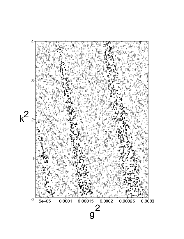
Figure 1: Band structure in the $k^{2}\times g^{2}$ space. Dark crosses indicate final energy above the cutoff (which, in this case, equals $100\,E_{0}$).

Figure 2: Fractal dimension $d_{f}$ of the first band shown in Fig. 1 versus the number of interacting fields $N$.

- (1) L. Kofman, A. Linde and A. A. Starobinsky, Phys. Rev. Lett. 73, 3195 (1994); ibid., 76,1011 (1996); Y. Shtanov, J. Traschen and R. Brandenberger, Phys. Rev. D51, 5438 (1995).
- (2) L. Kofman, A. Linde and A. A. Starobinsky, Phys. Rev. D56, 3258 (1997); D. Boyanovsky, H. J. de Vega, R. Holman and J. F. J. Salgado, Phys. Rev. D54, 7570 (1996).
- (3) S. E. Jorás and V. H. Cardenas, gr-qc/0108088.
- (4) G. Felder and L. Kofman, Phys. Rev. D63, 103503 (2001).
- (5) R. O. Ramos and F. A. R. Navarro, Phys. Rev. D62, 085016 (2000).
- (6) R. O. Ramos, Phys. Rev. D64, 123510 (2001).
- (7) M. Gleiser and R. O. Ramos, Phys. Rev. D50, 2441 (1994).
- (8) V. Zanchin, A. Maia, Jr., W. Craig and R. Brandenberger, Phys. Rev. D57, 4651 (1998).
- (9) V. Zanchin, A. Maia, Jr., W. Craig and R. Brandenberger, Phys. Rev. D60, 023505 (1999).
- (10) B. L. Hu, J. P. Paz and Y. Zhang, in The Origin of Structure in the Universe, edited by E. Gunzig and P. Nardone (Kluwer Academic, Norville, 1993); B. L. Hu, J. P. Paz and Y. Zhang, Phys. Rev. D45, 2843 (1993); ibid D47, 1576 (1993); E. Calzetta and B. L. Hu, Phys. Rev. D49, 6636 (1994); ibid D52, 6770 (1995); B. L. Hu and A. Matacz, Phys. Rev. D51, 1577 (1995); A. Matacz, Phys. Rev. D55, 1860 (1997).
- (11) M. Morikawa, Phys. Rev. D33, 3607 (1986).
- (12) S. A. Ramsey, B. L. Hu and A. M. Stylianopoulos, Phys. Rev. D57, 6003 (1998).
- (13) J. D. Barrow and J. Levin, Phys. Rev. Lett. 80, 656 (1998); N. J. Cornish and J. J. Levin, Phys. Rev. D53, 3022 (1996); Phys. Rev. D55, 7489 (1997).
- (14) K. Ferraz, G. Francisco, G. E. A. Matsas, Phys. Lett. A156, 407 (1991).
- (15) Y. Shtanov, J. Traschen and R. Brandenberger, Phys. Rev D51, 5438 (1995); F. Finelli and R. Brandenberger, Phys. Rev D62, 083502 (2000); Phys. Rev. Lett. 82, 1362 (1999).
- (16) A. Berera and R. O. Ramos, Phys. Rev. D63, 103509 (2001).
- (17) A. Berera, M. Gleiser and R. O. Ramos, Phys. Rev. D58, 123508 (1998).
- (18) K. Chou, Z. Su, B. Hao and L. Yu, Phys. Rep. 118, 1 (1985).
- (19) N. P. Landsman and Ch. G. van Weert, Phys. Rep. 145, 141 (1987).
- (20) R. Rivers, Path Integral Methods in Quantum Field Theory (Cambridge University Press, Cambridge 1987).
- (21) E. Ott, Chaos in Dynamical Systems (Cambridge University Press, Cambridge 1993).
- (22) L. G. S. Duarte, L. A. C. P. da Mota, H. P. de Oliveira, R. O. Ramos and J. E. Skea, Comp. Phys. Comm. 119, 256 (1999).
- (23) A. Berera, M. Gleiser and R. O. Ramos, Phys. Rev. Lett. 83, 264 (1999).
- (24) S. E. Jorás and R. O. Ramos, in preparation.