Abstract

The observation of charged lepton flavor non–conservation would be a clear signature of physics beyond the Standard Model. In particular, supersymmetric (SUSY) models introduce mixings in the sneutrino and the charged slepton sectors which could imply flavor–changing processes at rates accessible to upcoming experiments. In this paper we analyze the possibility to observe $Z\rightarrow\ell_{I}\ell_{J}$ in the GigaZ option of TESLA at DESY. We show that although models with SUSY masses above the current limits could predict a branching ratio ${\rm BR}(Z\rightarrow\mu e)$ accessible to the experiment, they would imply an unobserved rate of $\mu\rightarrow e\gamma$ and thus are excluded. In models with a small mixing angle between the first and the third (or the second and the third) slepton families GigaZ could observe $Z\rightarrow\tau\mu$ (or $Z\rightarrow\tau e$) consistently with present bounds on $\ell_{J}\rightarrow\ell_{I}\gamma$. In contrast, if the mixing angles between the three slepton families are large the bounds from $\mu\rightarrow e\gamma$ push these processes below the reach of GigaZ. We show that in this case the masses of the three slepton families must be strongly degenerated (with mass differences of order $10^{-3}$). We update the limits on the slepton mass insertions $\delta_{LL,RR,LR}$ and discuss the correlation between flavor changing and $g_{\mu}-2$ in SUSY models.

PACS numbers: 12.60.Jv, 13.35.-r, 13.38.Dg

1 Introduction

Lepton flavor violation (LFV) has been searched in several experiments. The current status in $\mu$ and $\tau$ decays is

$${\rm BR}(\mu\rightarrow e\gamma) < 1.2\times 10^{-11}\quad\cite[cite]{[\@@bibref{}{Brooks:1999pu}{}{}]}\;,$$

$${\rm BR}(\tau\rightarrow e\gamma) < 2.7\times 10^{-6}\quad\cite[cite]{[\@@bibref{}{Edwards:1996te}{}{}]}\;,$$

$${\rm BR}(\tau\rightarrow\mu\gamma) < 1.1\times 10^{-6}\quad\cite[cite]{[\@@bibref{}{Ahmed:1999gh}{}{}]}\;,$$ (1)

and

$${\rm BR}(\mu\rightarrow 3e) < 1.0\times 10^{-12}\quad\cite[cite]{[\@@bibref{}{Bellgardt:1987du}{}{}]}\;,$$

$${\rm BR}(\tau\rightarrow 3e) < 2.9\times 10^{-6}\quad\cite[cite]{[\@@bibref{}{Bliss:1997iq}{}{}]}\;,$$

$${\rm BR}(\tau\rightarrow 3\mu) < 1.9\times 10^{-6}\quad\cite[cite]{[\@@bibref{}{Bliss:1997iq}{}{}]}\;.$$ (2)

In $Z$ decays we have

$${\rm BR}(Z\rightarrow\mu e) < 1.7\times 10^{-6}\quad\cite[cite]{[\@@bibref{}{Akers:1995gz}{}{}]}\;,$$

$${\rm BR}(Z\rightarrow\tau e) < 9.8\times 10^{-6}\quad\cite[cite]{[\@@bibref{}{Akers:1995gz}{}{}]}\;,$$

$${\rm BR}(Z\rightarrow\tau\mu) < 1.2\times 10^{-5}\quad\cite[cite]{[\@@bibref{}{Abreu:1996mj}{}{}]}\;.$$ (3)

These observations are obviously in agreement with the Standard Model (SM), where lepton flavor number is (perturbatively) conserved.

On the other hand, neutrino oscillations are a first evidence of LFV. Small neutrino masses and mixings of order one suggest the existence of a new scale around $10^{12}$ GeV [9]. Massive neutrinos could be naturally accommodated within the SM (the so called $\nu$SM). The contributions from the light neutrino sector to other LFV processes, however, would be very small: BR$(\ell_{J}\rightarrow\ell_{I}\gamma)\raisebox{-3.69899pt}{~{}\shortstack{$<$ \\ [-0.07cm] $\sim$}}~{}10^{-48}$ and BR$(Z\rightarrow\ell_{I}\ell_{J})\raisebox{-3.69899pt}{~{}\shortstack{$<$ \\ [-0.07cm] $\sim$}}~{}10^{-54}$ [10]. In consequence, any experimental signature of LFV in the charged sector would be a clear signature of nonstandard physics.

In this paper we will study the implications of supersymmetry (SUSY) on $Z\rightarrow\ell_{I}\ell_{J}$. The GigaZ option of the TESLA Linear Collider project [12] could reduce the LEP bounds down to [13]

$${\rm BR}(Z\rightarrow\mu e) < 2.0\times 10^{-9}\;,$$

$${\rm BR}(Z\rightarrow\tau e) < \kappa\times 6.5\times 10^{-8}\;,$$

$${\rm BR}(Z\rightarrow\tau\mu) < \kappa\times 2.2\times 10^{-8}\;,$$ (4)

with $\kappa=0.2-1.0$. We will here explore the possibility that SUSY provides a signal accessible to GigaZ in consistency with current bounds from BR$(\ell_{J}\rightarrow\ell_{I}\gamma)$. Note that in SUSY models the branching ratio ${\rm BR}(\ell_{J}\rightarrow 3\ell_{I})\approx\alpha_{em}{\rm BR}(\ell_{J}\rightarrow\ell_{I}\gamma)$ will place weaker bounds on SUSY parameters (see Eqs. (1,2)) The conversion rate $\mu\rightarrow e$ on Ti gives also weaker bounds at current experiments, although this may change in the future (see [14] for a recent review).

We will concentrate on the minimal SUSY extension of the SM (MSSM) with R-parity and general soft SUSY–breaking terms. Related works on LFV in $Z$ decays in SUSY models study the MSSM [15] and a left–right SUSY model [16]. Several groups have analyzed other LFV processes in SUSY grand unified models with massive neutrinos (motivated by the atmospheric and solar neutrino anomalies [17]), or with R–parity violation [18]. There are also studies [19, 20] relating LFV $Z$ decays with other processes. Direct signals of lepton flavor non–conservation in slepton production at the LHC [21] and at future $e^{+}e^{-}$ or $\mu^{+}\mu^{-}$ colliders [22] have been also explored.

Other works on LFV $Z$ decays in alternative models include the SM with massive Dirac or Majorana neutrinos [10, 23], left–right symmetric models [24], models with a heavy $Z^{\prime}$ boson [25], two Higgs doublet models (2HDMs) [26] or technicolor [27].

2 Calculation

The most general vertex $V\bar{\ell}_{I}\ell_{J}$ coupling a (lepton) fermion current to a vector boson can be parametrized in terms of four form factors:

$${\cal M}=i\varepsilon^{\mu}_{V}\bar{u}_{\ell_{I}}(p_{2})\left[\gamma_{\mu}(F_{V}-F_{A}\gamma_{5})+(iF_{M}+F_{E}\gamma_{5})\sigma_{\mu\nu}q^{\nu}\right]u_{\ell_{J}}(p_{1})\;,$$ (5)

where $\varepsilon_{V}$ is the polarization vector ($\varepsilon_{V}\cdot q=0$) and $q=p_{2}-p_{1}$ is the momentum transfer. For an on–shell (massless) photon $F_{A}=0$, and, in addition, if $m_{I}\not=m_{J}$ then $F_{V}=0$. This implies that the flavor–changing process $\ell_{J}\rightarrow\ell_{I}\gamma$ is determined by (chirality flipping) dipole transitions only. In contrast, all form factors contribute to the decay of a $Z$ boson:

$${\rm BR}(Z\to\ell_{I}\ell_{J}) \equiv {\rm BR}(Z\to\bar{\ell}_{I}\ell_{J})+{\rm BR}(Z\to\ell_{I}\bar{\ell}_{J})$$ (6)

$$= \frac{\alpha_{W}^{3}M_{Z}}{48\pi^{2}\Gamma_{Z}}\left[|f_{L}|^{2}+|f_{R}|^{2}+\frac{1}{c^{2}_{W}}(|f_{M}|^{2}+|f_{E}|^{2})\right],$$

with $\alpha_{W}=g^{2}/(4\pi)$, $f_{L,R}=f_{V}\pm f_{A}$, $f_{V,A}\equiv-16\pi^{2}g^{-3}F_{V,A}$ and $f_{M,E}\equiv-16M_{W}\pi^{2}g^{-3}F_{M,E}$. We calculate (see Appendices A and B for details) these branching ratios in the MSSM.

Let us consider the case with two lepton families. Since SUSY is broken, fermion and scalar mass matrices will be diagonalized by different rotations in flavor space. After the diagonalization of the fermion sector we are left with a $2\times 2$ scalar matrix with 3 arbitrary parameters. We will assume that the rotation that diagonalizes the scalar matrix is maximal, $\theta=\pi/4$ (i.e. we assume no alignment between fermion and scalar fields; the amplitudes that we will calculate are proportional to $\sin 2\theta$). Our choice corresponds to a mass matrix with identical diagonal terms. Taking

$${\bf m}^{2}=\tilde{m}^{2}\pmatrix{\sqrt{1+\delta^{2}}&\delta\cr\delta&\sqrt{1+\delta^{2}}\cr}\;,$$ (7)

the two mass eigenvalues are

$$\tilde{m}_{1,2}^{2}=\tilde{m}^{2}(\sqrt{1+\delta^{2}}\mp\delta)\;.$$ (8)

In this parametrization $\tilde{m}^{2}=\tilde{m}_{1}\tilde{m}_{2}$ characterizes the SUSY–breaking scale and $\delta=(\tilde{m}_{2}^{2}-\tilde{m}_{1}^{2})/(2\tilde{m}^{2})$ the mass splitting between the two families. $\delta$ is also responsible for any flavor–changing process: $\delta=0$ corresponds to the flavor–conserving case, $\delta\ll 1$ can be treated as a non–diagonal mass insertion, and $\delta\rightarrow\infty$ gives $\tilde{m}_{2}^{2}\rightarrow\infty$ (a decoupled second family). The last case implies a maximum flavor–changing rate [15, 16].

To analyze the general case with three lepton families we will consider two scenarios. First, we will follow the usual approach [28] where the influence of a nondiagonal term $\tilde{\delta}^{IJ}$ is calculated putting the rest to zero. This implies that the slepton family $\ell_{K\not=I,J}$ does not mix with $\ell_{I}$ and $\ell_{J}$ ($\theta_{IK}=\theta_{JK}=0$), which reduces the problem to the two family case discussed above. This approximation is only justified if the off–diagonal terms satisfy $\tilde{\delta}^{IK}\tilde{\delta}^{KJ}<\tilde{\delta}^{IJ}$ or, in terms of mixing angles and mass differences, if

$$\left({\tilde{m}_{I}^{2}-\tilde{m}_{K}^{2}\over\tilde{m}_{I}^{2}+\tilde{m}_{K}^{2}}\sin\theta_{IK}\right)\left({\tilde{m}_{K}^{2}-\tilde{m}_{J}^{2}\over\tilde{m}_{K}^{2}+\tilde{m}_{J}^{2}}\sin\theta_{JK}\right)\raisebox{-3.69899pt}{~{}\shortstack{$<$ \\ [-0.07cm] $\sim$}}~{}{\tilde{m}_{I}^{2}-\tilde{m}_{J}^{2}\over\tilde{m}_{I}^{2}+\tilde{m}_{J}^{2}}\sin\theta_{IJ}\;.$$ (9)

We will then discuss a second scenario with maximal mixing between the three slepton families: $\theta_{12}=\theta_{23}=\theta_{13}=\pi/4$. Large mixings are suggested by the observation of solar and atmospheric neutrino oscilations (note, however, that the non observation of $\nu_{e}-\nu_{\tau}$ oscilations in CHOOZ [29] could suggest $\theta_{13}\raisebox{-3.69899pt}{~{}\shortstack{$<$ \\ [-0.07cm] $\sim$}}~{}0.1$). We will use $\delta^{IJ}$ to parametrize the mass difference between $\ell_{I}$ and $\ell_{J}$: $\delta^{IJ}\equiv(\tilde{m}_{J}^{2}-\tilde{m}_{I}^{2})/(2\tilde{m}_{1}^{2})$, where $\tilde{m}_{1}^{2}$ is the mass of the lightest slepton family.

The relevant parameters for the calculation will then be the masses and mixings of charginos and neutralinos, the masses of the six (‘left’ and ‘right’ handed) charged sleptons, and the masses of the three sneutrinos. When we evaluate the contribution of each $\delta^{IJ}$ to $Z\rightarrow\ell_{I}\ell_{J}$ and $\ell_{J}\rightarrow\ell_{I}\gamma$ setting all the other to zero we will have three independent parameters $\delta^{\tilde{\nu}\,IJ}_{LL}$ in the sneutrino sector and nine $\delta^{\tilde{\ell}\,IJ}_{LL}$, $\delta^{\tilde{\ell}\,IJ}_{RR}$ and $\delta^{\tilde{\ell}\,IJ}_{LR}$ in the charged slepton sector. In the case of maximal mixing between the three slepton families there will be two independent mass differences $\delta^{\tilde{\nu}\,IJ}_{LL}$ and four $\delta^{\tilde{\ell}\,IJ}_{LL}$, $\delta^{\tilde{\ell}\,IJ}_{RR}$ (note that in this case $\delta^{23}=\delta^{13}-\delta^{12}$).

In our analysis we will not assume any (grand unification) relation between slepton masses. For each non–zero choice of $\delta^{IJ}$ it is straightforward to obtain and diagonalize the mass matrix that corresponds to a maximal rotation angle (see Appendix B). Our results should coincide with the ones obtained in the limit of small mass difference using the mass insertion method, but they are also valid for any large value of $\delta^{IJ}$.

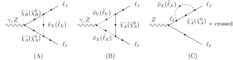
Figure 1: SUSY contributions to the LFV processes $Z\to\ell_{I}\ell_{J}$ and $\ell_{J}\to\ell_{I}\gamma$.

The process $Z\rightarrow\ell_{I}\ell_{J}$ goes through the diagrams in Fig. 1. Box diagrams mediating $e^{+}e^{-}\to\ell_{I}\ell_{J}$ introduce a small correction of order $\Gamma_{Z}/M_{Z}\approx\alpha$. Analogous diagrams describe $\ell_{J}\rightarrow\ell_{I}\gamma$. The inclusion of the contributions of the third type is essential to cancel ultraviolet divergences (they are related to counterterms by Ward identities). Diagrams with neutralinos in (A) or sneutrinos in (B) do not couple to the photon. The diagrams of type (C) do not give dipole contributions.

Figure 2: BR$(Z\to\mu e)$ (lower curves) and BR$(\mu\to e\gamma)$ (upper curves) as a function of the lightest scalar mass $\tilde{m}_{1}$ for $\tan\beta=2$ and the different $\delta^{12}$. Solid lines correspond to $M_{2}=150$ GeV and $\mu=-500$ GeV and dashed lines to $M_{2}=\mu=150$ GeV.

Table 1: Approximate lower bounds on SUSY mass parameters based on [30]. Note that, for negligible scalar trilinears, $m_{\tilde{\nu}}^{2}=m_{\tilde{\ell}_{L}}^{2}+M^{2}_{Z}c^{2}_{W}\cos 2\beta$, and the bounds on $m_{\tilde{\nu}}$ and $m_{\tilde{\ell}_{L}}$ are correlated. For instance: $m_{\tilde{\nu}}>65\ (40)\ \mbox{GeV for}\ \tan\beta=2\ (50)$.

lightest slepton $(\tilde{m}_{1})$	$m_{\tilde{\nu}}\geq 45$ GeV
	$m_{\tilde{\ell}_{L,R}}\geq 90$ GeV
lightest chargino	$m_{\tilde{\chi}^{+}_{1}}\geq 75$ GeV, if $m_{\tilde{\nu}}>m_{\chi^{+}_{1}}$
	$m_{\tilde{\chi}^{+}_{1}}\geq 45$ GeV, otherwise
lightest neutralino	$m_{\tilde{\chi}^{0}_{1}}\geq 35\mbox{ GeV}$

Due to the weaker experimental bounds (in Table 1) on sneutrino masses, the dominant contributions to $Z\rightarrow\ell_{I}\ell_{J}$ will come from the diagrams mediated by chargino–sneutrino (see Fig. 2). Note that sneutrino masses can be substantially lighter than charged slepton masses for large $\tan\beta$ and light SUSY–breaking masses,

$$m^{2}_{\tilde{\nu}} \approx m^{2}_{L}+{1\over 2}M_{Z}^{2}\cos 2\beta\;,$$

$$m^{2}_{\tilde{\ell}_{L}} \approx m^{2}_{L}+\left(-{1\over 2}+s_{W}^{2}\right)M_{Z}^{2}\cos 2\beta\;,$$ (10)

which tends to increase the maximum relative contribution of chargino–sneutrino diagrams.

We would like to emphasize that our results will depend on contributions with opposite signs that often cancel when varying a parameter. For example, one would expect that the process $Z\rightarrow\ell_{I}\ell_{J}$ is optimized for light slepton masses. However, we observe frequently the opposite effect. Its branching ratio can increase by raising the mass of the sleptons up to values of 500 GeV, and only at masses above $1-2$ TeV the asymptotic regime is reached (see Fig. 2). These cancellations give a one or two orders of magnitude uncertainty to any naive estimate, and underline the need for a complete calculation like the one presented here.

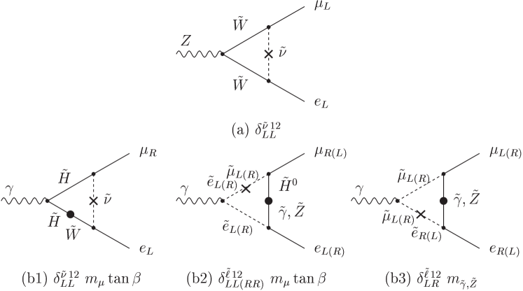
Figure 3: Dominant diagrams contributing to (a) $Z\to\mu e$ and (b) $\mu\to e\gamma$, in terms of gauginos, higgsinos and current eigenstates, showing the approximate linear dependence on the flavor–changing mass insertions $\delta^{12}$ (crosses), the fermion mass insertions (big dots) and $\tan\beta$.

We give in Fig. 3 the dominant diagrams in terms of gauginos, current eigenstates and mass insertions, specifying the chirality of the external fermion. All the diagrams contributing to $\ell_{J}\rightarrow\ell_{I}\gamma$ except for the last one grow with $\tan\beta$.

3 Results

3.1 $Z\rightarrow\ell_{I}\ell_{J}$ at TESLA GigaZ

Let us consider the process $Z\rightarrow\ell_{I}\ell_{J}$ uncorrelated from other LFV processes. For SUSY masses above the current limits it is possible to have $Z\rightarrow\mu e;\tau e;\tau\mu$ at the reach of GigaZ. The maximun rate is obtained when the second slepton $\tilde{\ell}_{J}$ is very heavy (i.e. $\delta^{IJ}\rightarrow\infty$). The largest contribution comes from virtual sneutrino–chargino diagrams (all other contributions are at least one order of magnitude smaller). It gives ${\rm BR}(Z\rightarrow\ell_{I}\ell_{J})$ from $2.5\times 10^{-8}$ for $\tan\beta=2$ to $7.5\times 10^{-8}$ for $\tan\beta=50$, practically independent of the lepton masses. The variation is due to the mild dependence of chargino and sneutrino masses on $\tan\beta$. These branching ratios are above the values given in Eq. (4). We find that a branching ratio larger than $2\times 10^{-9}$ ($2\times 10^{-8}$) can be obtained with sneutrino masses of up to 305 GeV (85 GeV) and chargino masses of up to 270 GeV (105 GeV).

Most of these values of ${\rm BR}(Z\rightarrow\ell_{I}\ell_{J})$, however, are correlated with an experimentally excluded rate of $\ell_{J}\rightarrow\ell_{I}\gamma$. We give below the results in the two scenarios (independent off-diagonal terms and maximal mixing of the three flavors) described in the previous section.

(i) We separate the contribution of each $\delta^{IJ}$ setting all the other to zero. For the first two families, after scanning for all the parameters in the model we find that ${\rm BR}(\mu\rightarrow e\gamma)<1.2\times 10^{-11}$ implies ${\rm BR}(Z\rightarrow\mu e)<1.5\times 10^{-10}$, which is below the reach of GigaZ.

Figure 4: BR$(Z\to\tau\mu)$ and $BR(\tau\to\mu\gamma)$ as a function of the lightest sneutrino mass ($\tilde{m}_{1}$) with the other one decoupled ($\delta^{\tilde{\nu}\,23}_{LL}\to\infty$), in several SUSY scenarios at the reach of GigaZ.

A more promising result is obtained for the processes involving the $\tau$ lepton. It turns out (see also next section) that the bounds from $\tau\rightarrow\ell_{I}\gamma$ can be avoided while still keeping a rate of $Z\rightarrow\tau\ell_{I}$ at the reach of the best GigaZ projection (see Fig. 4). In particular, for large $\delta^{\tilde{\nu}\,13}_{LL}$ (or $\delta^{\tilde{\nu}\,23}_{LL}$) and a light sneutrino (of around 70 GeV) we get ${\rm BR}(Z\rightarrow\tau e)\approx 1.6\times 10^{-8}$ for ${\rm BR}(\tau\rightarrow e\gamma)\approx 3.5\times 10^{-8}$, which is two orders of magnitude below current limits (with similar results for ${\rm BR}(Z\rightarrow\tau\mu)$ and ${\rm BR}(\tau\rightarrow\mu\gamma)$). This result is due to the sneutrino–chargino diagram. The contributions due to charged slepton mixing are essentially different in the sense that they saturate the experimental bound to $\tau\rightarrow\ell_{I}\gamma$ giving a small effect (at most, one order of magnitude below the reach of GigaZ) in $Z\rightarrow\tau\ell_{I}$. We obtain events at the reach of GigaZ with lightest sneutrino masses from 55 to 215 GeV, lightest chargino from 75 to 100 GeV, and $\tan\beta$ up to 7.

(ii) In the case with maximal mixing between the three slepton flavors it is not consistent to take $\delta^{IJ}\not=0$ and $\delta^{IK}=\delta^{KJ}=0$. In terms of slepton mass differences, only two of the three mass differences are independent ($\delta^{23}=\delta^{13}-\delta^{12}$). In terms of off-diagonal terms $\tilde{\delta}^{IJ}$ in the mass matrix, for maximal mixing only one of them can be put to zero. Note that in this case the non-observation of $\mu\rightarrow e\gamma$ will constraint all the $\delta^{IJ}$ parameters, not only $\delta^{12}$: a non-diagonal $\tilde{\delta}^{12}$ mass insertion would be generated through a $\tilde{\delta}^{13}$ followed by a $\tilde{\delta}^{32}$. In fact, we find that the constraints from $\tau\rightarrow e\gamma;\mu\gamma$ are always weaker than the one from $\mu\rightarrow e\gamma$. A branching ratio ${\rm BR}(\mu\rightarrow e\gamma)<1.2\times 10^{-11}$ implies ${\rm BR}(Z\rightarrow\mu e;\;\tau e;\;\tau\mu)\raisebox{-3.69899pt}{~{}\shortstack{$<$ \\ [-0.07cm] $\sim$}}~{}10^{-9}$, and the three lepton flavor violating decays of the $Z$ boson would be out of the reach of Giga Z.

3.2 Bounds on $\delta^{IJ}$ from $\ell_{J}\rightarrow\ell_{I}\gamma$

The bounds on the $\delta^{IJ}$ parameters establish how severe is the flavor problem in the lepton sector of the MSSM. We will update them here, including the sneutrino–chargino contributions neglected in previous works [28] and the general slepton–neutralino contributions (photino diagrams are typically subdominant as pointed out by Ref. [31]). In addition, we also consider the case of maximum mixing between the three slepton families.

Table 2: Bounds on the $\delta^{12}$s from BR$(\mu\to e\gamma)<1.2\times 10^{-11}$ in different SUSY scenarios assuming no mixing with the third family. The bounds on $\delta^{IJ}$ in the case of three family mixing can be read from these ones (see text).

$\delta^{\tilde{\nu}\,12}_{LL}$	$\tilde{m}_{1}$	$M_{2}$	$\mu=-500$	$\mu=-150$	$\mu=150$	$\mu=500$
	100	150	$14\times 10^{-3}$	$1.0\times 10^{-3}$	$0.3\times 10^{-3}$	$1.0\times 10^{-3}$
$\tan\beta=2$		500	$33\times 10^{-3}$	$3.0\times 10^{-3}$	$1.7\times 10^{-3}$	$13\times 10^{-3}$
	500	150	$3.7\times 10^{-3}$	$1.1\times 10^{-3}$	$1.2\times 10^{-3}$	$1.7\times 10^{-3}$
		500	$7.3\times 10^{-3}$	$2.6\times 10^{-3}$	$2.3\times 10^{-3}$	$4.1\times 10^{-3}$
	100	150	$9.3\times 10^{-5}$	$2.1\times 10^{-5}$	$2.0\times 10^{-5}$	$8.6\times 10^{-5}$
$\tan\beta=50$		500	$80\times 10^{-5}$	$9.0\times 10^{-5}$	$8.8\times 10^{-5}$	$77\times 10^{-5}$
	500	150	$9.7\times 10^{-5}$	$4.5\times 10^{-5}$	$4.5\times 10^{-5}$	$9.4\times 10^{-5}$
		500	$22\times 10^{-5}$	$9.6\times 10^{-5}$	$9.5\times 10^{-5}$	$21\times 10^{-5}$
$\delta^{\tilde{\ell}\,12}_{LL}$	$\tilde{m}_{1}$	$M_{2}$	$\mu=-500$	$\mu=-150$	$\mu=150$	$\mu=500$
	100	150	$7.5\times 10^{-3}$	$2.6\times 10^{-3}$	$1.7\times 10^{-3}$	$5.0\times 10^{-3}$
$\tan\beta=2$		500	$84\times 10^{-3}$	$11\times 10^{-3}$	$7.0\times 10^{-3}$	$41\times 10^{-3}$
	500	150	$14\times 10^{-3}$	$8.5\times 10^{-3}$	$0.12$	$32\times 10^{-3}$
		500	$24\times 10^{-3}$	$20\times 10^{-3}$	$32\times 10^{-3}$	$26\times 10^{-3}$
	100	150	$2.4\times 10^{-4}$	$0.8\times 10^{-4}$	$0.8\times 10^{-4}$	$2.4\times 10^{-4}$
$\tan\beta=50$		500	$24\times 10^{-4}$	$3.5\times 10^{-4}$	$3.4\times 10^{-4}$	$23\times 10^{-4}$
	500	150	$7.4\times 10^{-4}$	$6.4\times 10^{-4}$	$6.9\times 10^{-4}$	$7.6\times 10^{-4}$
		500	$9.7\times 10^{-4}$	$9.6\times 10^{-4}$	$9.8\times 10^{-4}$	$9.7\times 10^{-4}$
$\delta^{\tilde{\ell}\,12}_{RR}$	$\tilde{m}_{1}$	$M_{2}$	$\mu=-500$	$\mu=-150$	$\mu=150$	$\mu=500$
	100	150	$4.2\times 10^{-3}$	$1.5\times 10^{-3}$	$1.8\times 10^{-3}$	$3.7\times 10^{-3}$
$\tan\beta=2$		500	$11\times 10^{-3}$	$3.2\times 10^{-3}$	$2.5\times 10^{-3}$	$8.3\times 10^{-3}$
	500	150	$22\times 10^{-3}$	$10\times 10^{-3}$	$22\times 10^{-3}$	$0.33$
		500	$19\times 10^{-3}$	$12\times 10^{-3}$	$0.33$	$35\times 10^{-3}$
	100	150	$1.6\times 10^{-4}$	$0.6\times 10^{-4}$	$0.6\times 10^{-4}$	$1.5\times 10^{-4}$
$\tan\beta=50$		500	$3.8\times 10^{-4}$	$1.1\times 10^{-4}$	$1.1\times 10^{-4}$	$3.8\times 10^{-4}$
	500	150	$16\times 10^{-4}$	$13\times 10^{-4}$	$15\times 10^{-4}$	$17\times 10^{-4}$
		500	$9.4\times 10^{-4}$	$8.1\times 10^{-4}$	$8.7\times 10^{-4}$	$9.6\times 10^{-4}$
$\delta^{\tilde{\ell}\,12}_{LR}$	$\tilde{m}_{1}$	$M_{2}$	$\mu=-500$	$\mu=-150$	$\mu=150$	$\mu=500$
	100	150	$1.6\times 10^{-6}$	$1.5\times 10^{-6}$	$1.6\times 10^{-6}$	$1.7\times 10^{-6}$
$\tan\beta=2$		500	$4.5\times 10^{-6}$	$4.4\times 10^{-6}$	$4.7\times 10^{-6}$	$4.6\times 10^{-6}$
	500	150	$1.3\times 10^{-6}$	$1.2\times 10^{-6}$	$1.2\times 10^{-6}$	$1.2\times 10^{-6}$
		500	$7.6\times 10^{-6}$	$7.5\times 10^{-6}$	$7.6\times 10^{-6}$	$7.7\times 10^{-6}$
	100	150	$1.6\times 10^{-6}$	$1.5\times 10^{-6}$	$1.6\times 10^{-6}$	$1.6\times 10^{-6}$
$\tan\beta=50$		500	$4.5\times 10^{-6}$	$4.5\times 10^{-6}$	$4.6\times 10^{-6}$	$4.5\times 10^{-6}$
	500	150	$1.3\times 10^{-6}$	$1.2\times 10^{-6}$	$1.2\times 10^{-6}$	$1.3\times 10^{-6}$
		500	$7.7\times 10^{-6}$	$7.6\times 10^{-6}$	$7.6\times 10^{-6}$	$7.7\times 10^{-6}$

The limits come exclusively from the process $\ell_{J}\rightarrow\ell_{I}\gamma$. To estimate the MSSM prediction we combine low and high values of the relevant parameters: $\tan\beta=2;50$, $\tilde{m}_{1}=100;500$ GeV, and the gaugino and higgsino mass parameters $M_{2}=150;500$ GeV and $\mu=\pm 150;\pm 500$ GeV.

(i) The results for the case with a decoupled family are summarized in Table 2. We include the bounds from $\mu\rightarrow e\gamma$ to $\delta^{\tilde{\nu}\,12}_{LL}$, $\delta^{\tilde{\ell}\,12}_{LL}$, $\delta^{\tilde{\ell}\,12}_{RR}$ and $\delta^{\tilde{\ell}\,12}_{LR}$. A $\delta\approx 10^{-3}$ implies a 1‰ degeneracy between the two slepton masses. We observe that the degeneracy between the selectron and the smuon is required even for large SUSY masses, and it must be stronger if $\tan\beta$ is large, as expected from the diagrams in Fig. 3. The small values of $\delta^{\tilde{\ell}\,12}_{LR}$, around $10^{-6}$, imply just that the scalar trilinears, usually assumed proportional to the Yukawa couplings, are small. Particularly weak bounds on the $\delta$’s (bold faced in Table 2) are obtained when approaching a dip of the curves in Fig. 2. This occurs for certain values of the SUSY parameters due to cancellations of the contributions of the various particles running in the loops.

The experimental bounds on the mass differences involving the third family are much weaker. They come from $\tau\rightarrow\ell_{I}\gamma$ (and not from $\mu\rightarrow e\gamma$), since in this case we are asuming that the mixing with $\ell_{J}$ ($J\not=I,3$) is negligible. For small $\tan\beta$ we find no bounds on any $\delta^{I3}$ (except for $\delta^{\tilde{\ell}\,I3}_{LR}$). For large $\tan\beta$ the bounds are (depending on the values of the SUSY–breaking masses) $\delta^{\tilde{\nu}\,I3}_{LL}=0.03\;{\rm to}\;1.3$; $\delta^{\tilde{\ell}\,I3}_{LL}=0.14\;{\rm to}\;\infty$; and $\delta^{\tilde{\ell}\,I3}_{RR}=0.11\;{\rm to}\;\infty$. For the $LR$ mass insertions, we find $\delta^{\tilde{\ell}\,I3}_{LR}=0.05\;{\rm to}\;\infty$, independent of $\tan\beta$. This results improve the bounds obtained in Ref. [28], in particular, the ones involving the second and third lepton families.

(ii) As explained before, if the three slepton families are maximally mixed (as suggested by the experiments on neutrino oscilations) then the strongest bounds on all the slepton mass differences come from $\mu\rightarrow e\gamma$ exclusively. As we will see, however, the bounds can be read directly from Table 2, since the small values obtained for $\delta^{12}$ admit an analysis based on mass insertions. Let us first suppose that the first and second sneutrino families are degenerated ($\delta^{\tilde{\nu}\,12}_{LL}=0$). Then a mass difference $\delta^{\tilde{\nu}\,13}_{LL}=\delta^{\tilde{\nu}\,23}_{LL}=\delta$ generates an off-diagonal mass term (see Appendix B3) $\tilde{\delta}^{\tilde{\nu}\,12}_{LL}=\delta/4$. In consecuence, the degree of mass degeneracy with the third family ($\delta$) imposed by $\mu\rightarrow e\gamma$ is just four times the value given in Table 2. We have checked numerically that this estimate is quite accurate. Analogously, the bounds on $\delta^{\tilde{\nu}\,12}_{LL}=\delta^{\tilde{\nu}\,13}_{LL}$ when $\delta^{\tilde{\nu}\,23}_{LL}=0$ and on $\delta^{\tilde{\nu}\,12}_{LL}=\delta^{\tilde{\nu}\,23}_{LL}$ when $\delta^{\tilde{\nu}\,13}_{LL}=0$ are respectively two and four times the values in Table 2. In the same way we can read there the bounds on $\delta^{\tilde{\ell}\,IJ}_{LL}$ and $\delta^{\tilde{\ell}\,IJ}_{RR}$, which establish the degree of mass degeneracy between the three families of charged sleptons.

3.3 Lepton flavor violation and $g_{\mu}-2$

Finally we would like to comment on the relation between $\mu\rightarrow e\gamma$ and the muon anomalous magnetic dipole moment. See Ref. [32] for more exhaustive analyses of the constraints on lepton flavor violation in the MSSM from the muon anomalous magnetic moment measurement. A $g_{\mu}-2$ correction would be generated by the diagrams in Fig. 3b if no mass insertions $\delta^{\tilde{\nu}\,IJ}_{LL}$, $\delta^{\tilde{\ell}\,IJ}_{LL}$, $\delta^{\tilde{\ell}\,IJ}_{RR}$ are included and $\delta^{\tilde{\ell}\,IJ}_{LR}$ is replaced by $\delta^{\tilde{\ell}\,22}_{LR}$. In this sense, $g_{\mu}-2$ is a normalization of the branching ratio BR$(\ell_{J}\rightarrow\ell_{I}\gamma)$ for processes changing the muon flavor.

Figure 5: Total SUSY contribution to the muon anomalous magnetic dipole moment as a function of the sneutrino mass with $m_{L}=m_{R}$, in the same SUSY scenarios as in Fig. 4.

We plot in Fig. 5 the value of $a_{\mu}=(g_{\mu}-2)/2$ for the SUSY parameters in the region accessible to GigaZ not excluded by $\tau\rightarrow\mu\gamma$, taking for simplicity equal soft–breaking terms $m_{L}=m_{R}$ (they would not very different, for example, assuming left–right unification at the GUT scale). We obtain, in agreement with [33], positive or negative contributions correlated with the sign of the Higgsino mass parameter $\mu$ and similar in size to the weak corrections. The recently revised SM prediction [34], $a^{\rm SM}_{\mu}=11\ 659\ 179.2\ (9.4)\times 10^{-10}$, compared to the world average after the last data from the Brookhaven E821 experiment [35], $a^{\rm exp}_{\mu}=11\ 659\ 202.3\ (15.1)\times 10^{-10}$, exhibits a 1.4$\sigma$ discrepancy: $\delta a_{\mu}=a^{\rm exp}_{\mu}-a^{\rm SM}_{\mu}=(23.1\pm 16.9)\times 10^{-10}$. This indicates that the muon dipole moment may still need non–standard contributions of positive sign. In any case, the MSSM contribution $\delta a^{\rm SUSY}_{\mu}$ is bounded at two standard deviations by the dotted lines in Fig. 5. Only the regions with heavier masses in the scenarios of Fig. 4 are favored.

Figure 6: Total SUSY contribution to the muon anomalous magnetic dipole moment as a function of the sneutrino mass, with $m_{L}=m_{R}$.

Fig. 6 shows the muon anomalous magnetic moment for the different sets of SUSY parameters employed to explore the muon LFV decay in Table 2. Low values of $\tan\beta$ and positive values of $\mu$ are preferred by $g_{\mu}-2$, which implies less stringent bounds on the $\delta$ insertions parametrizing the flavor–changing lepton decays.

4 Conclusions

SUSY models introduce LFV corrections which are proportional to slepton mass squared differences. We have shown that the non–observation of $\mu\rightarrow e\gamma$ implies around a 1‰ degeneracy between the masses of the sleptons in the first two families. Once this degeneracy is imposed, the rate of $Z\rightarrow\mu e$ is always below the limits to be explored at GigaZ. Moreover, if the mixing between the three slepton families is large then also the third family must be (at the 1‰) degenerated, and the processes $Z\rightarrow\tau e;\;\tau\mu$ will not be observed at the GigaZ. The degeneracy between the lightest slepton families could be justified by the weakness of its Yukawa couplings, but for the third family it should put constraints on definite SUSY models.

In contrast, if the mixing between the third and the first slepton families is small, then the third family could be much heavier than the other two and there would be no flavor problem in the slepton sector (the bounds would come only from $\tau\rightarrow\mu\gamma$, not from $\mu\rightarrow e\gamma$). In this case, if the GigaZ option of TESLA reaches its best projected sensitivity it could observe $Z\rightarrow\tau\mu$ coming from the virtual exchange of wino–sneutrino.

Acknowledgments
JII acknowledges the Theory Group of DESY Zeuthen and MM the Institute for Nuclear Research (Moscow) for their kind hospitality. We thank F. del Aguila, A. Bueno, D. Gorbunov, J. Prades and T. Riemann for useful discussions. This work has been supported by CICYT, Junta de Andalucía and the European Union under contracts FPA2000-1558, FQM-101 and HPRN-CT-2000-00149, respectively.

Note added
After the completion of this paper, new data from BNL $g-2$ experiment [42] appeared confirming the previous measurement with twice the precision. The discrepancy with the SM prediction is now more significant, up to $2.6\sigma$. There are also new experimental bounds on $\tau\to\mu\gamma$ [43]. The new data do not introduce any qualitative changes in our results.

Appendix A Generic expressions at one loop for $Z\bar{\ell}_{I}\ell_{J}$

A.1 Feynman rules in terms of generic vertex couplings

Let $f$ be a fermion, $\phi$ a scalar field and $P_{R,L}=(1\pm\gamma_{5})/2$. The Feynman rules for the three vertex topologies needed are:

$\bullet$ Vertex $Z\bar{f}_{A}f_{B}$	:	$ig\gamma^{\mu}(g^{L}_{AB}P_{L}+g^{R}_{AB}P_{R})\;,$
$\bullet$ Vertex $Z\phi_{X}^{\dagger}(p_{2})\phi_{Y}(p_{1})$	:	$igG_{XY}(p_{1}+p_{2})^{\mu}\;,$
$\bullet$ Vertex $\phi_{X}^{\dagger}\bar{f}_{A}f_{I}$	:	$ig(c^{L}_{IAX}P_{L}+c^{R}_{IAX}P_{R})\;.$

A.2 Invariant amplitude

The most general invariant amplitude for on–shell external legs is

$${\cal M}=-ig\frac{\alpha_{W}}{4\pi}\varepsilon^{\mu}_{Z}\bar{u}_{\ell_{I}}(p_{2})\left[\gamma_{\mu}(f_{V}-f_{A}\gamma_{5})+\frac{\sigma_{\mu\nu}q^{\nu}}{M_{W}}(if_{M}+f_{E}\gamma_{5})\right]u_{\ell_{J}}(p_{1})\;.$$ (11)

Let us introduce the squared mass ratios $\lambda_{n}=m^{2}_{n}/M^{2}_{W}$ and the dimensionless two– and three–point one–loop integrals

$${\mathbb{B}}_{1}(\lambda_{0},\lambda_{1}) \equiv B_{1}(0;m^{2}_{0},m^{2}_{1})\;,$$ (12)

$${\mathbb{C}}_{..}(\lambda_{0},\lambda_{1},\lambda_{2}) \equiv M^{2}_{W}\ C_{..}(0,M^{2}_{Z},0;m^{2}_{0},m^{2}_{1},m^{2}_{2})\;,$$ (13)

from the usual tensor integrals [36, 37],

$$B^{\mu}(p^{2};m^{2}_{0},m^{2}_{1}) = p^{\mu}B_{1}\;,$$ (14)

$$C^{\mu}(p^{2}_{1},q^{2},p^{2}_{2};m^{2}_{0},m^{2}_{1},m^{2}_{2}) = p^{\mu}_{1}C_{11}\!+\!p^{\mu}_{2}C_{12}\;,$$ (15)

$$C^{\mu\nu}(p^{2}_{1},q^{2},p^{2}_{2};m^{2}_{0},m^{2}_{1},m^{2}_{2}) = p^{\mu}_{1}p^{\nu}_{1}C_{21}+p^{\mu}_{2}p^{\nu}_{2}C_{22}+(p^{\mu}_{1}p^{\nu}_{2}+p^{\mu}_{2}p^{\nu}_{1})C_{23}+g^{\mu\nu}M^{2}_{W}C_{24}\;.$$ (16)

Note that ${\mathbb{C}}_{0}$, ${\mathbb{C}}_{23}$, ${\mathbb{C}}_{24}$, ${\mathbb{C}}_{11}+{\mathbb{C}}_{12}$ and ${\mathbb{C}}_{21}+{\mathbb{C}}_{22}$ are symmetric under the replacements $\lambda_{1}\leftrightarrow\lambda_{2}$, while ${\mathbb{C}}_{11}-{\mathbb{C}}_{12}$ and ${\mathbb{C}}_{21}-{\mathbb{C}}_{22}$ are antisymmetric. The form factors for each type of diagrams (Fig. 1) are:

$\bullet$ Diagram of type A:

$$f_{L}^{\chi\chi s} = \sum_{XAB}\Bigg{\{}g^{L}_{AB}c^{L^{*}}_{IAX}c^{L}_{JBX}\ \sqrt{\lambda_{A}\lambda_{B}}\ {\mathbb{C}}_{0}(\lambda_{X},\lambda_{A},\lambda_{B})$$ (17)

$$+g^{R}_{AB}c^{L^{*}}_{IAX}c^{L}_{JBX}\ \Bigg{[}\lambda_{Z}\ {\mathbb{C}}_{23}(\lambda_{X},\lambda_{A},\lambda_{B})-2\ {\mathbb{C}}_{24}(\lambda_{X},\lambda_{A},\lambda_{B})+\frac{1}{2}\Bigg{]}\Bigg{\}}\;,$$

$$f_{R}^{\chi\chi s} = f_{L}^{\chi\chi s}\ (\ L\leftrightarrow R\ )\;,$$ (18)

$$f_{M}^{\chi\chi s} = \sum_{XAB}\Bigg{\{}\frac{\sqrt{\lambda_{J}}}{2}\ [(g^{R}_{AB}c^{L^{*}}_{IAX}c^{L}_{JBX}+g^{L}_{AB}c^{R^{*}}_{IAX}c^{R}_{JBX})+(I\leftrightarrow J)^{*}]$$ (19)

$$\hskip 51.21495pt\times[{\mathbb{C}}_{11}(\lambda_{X},\lambda_{A},\lambda_{B})+{\mathbb{C}}_{21}(\lambda_{X},\lambda_{A},\lambda_{B})+{\mathbb{C}}_{23}(\lambda_{X},\lambda_{A},\lambda_{B})]$$

$$\hskip 22.76219pt+\frac{\sqrt{\lambda_{A}}}{2}\ [(g^{L}_{AB}c^{L^{*}}_{IAX}c^{R}_{JBX}+g^{R}_{AB}c^{R^{*}}_{IAX}c^{L}_{JBX})+(I\leftrightarrow J)^{*}]\ {\mathbb{C}}_{12}(\lambda_{X},\lambda_{A},\lambda_{B})\Bigg{\}}\;,$$

$$if_{E}^{\chi\chi s} = \sum_{XAB}\Bigg{\{}\frac{\sqrt{\lambda_{J}}}{2}\ [(g^{R}_{AB}c^{L^{*}}_{IAX}c^{L}_{JBX}-g^{L}_{AB}c^{R^{*}}_{IAX}c^{R}_{JBX})-(I\leftrightarrow J)^{*}]$$ (20)

$$\hskip 51.21495pt\times[{\mathbb{C}}_{11}(\lambda_{X},\lambda_{A},\lambda_{B})+{\mathbb{C}}_{21}(\lambda_{X},\lambda_{A},\lambda_{B})+{\mathbb{C}}_{23}(\lambda_{X},\lambda_{A},\lambda_{B})]$$

$$\hskip 22.76219pt+\frac{\sqrt{\lambda_{A}}}{2}\ [(g^{L}_{AB}c^{L^{*}}_{IAX}c^{R}_{JBX}-g^{R}_{AB}c^{R^{*}}_{IAX}c^{L}_{JBX})-(I\leftrightarrow J)^{*}]\ {\mathbb{C}}_{12}(\lambda_{X},\lambda_{A},\lambda_{B})\Bigg{\}}\;.$$

$\bullet$ Diagram of type B:

$$f_{L}^{ss\chi} = -2\sum_{AXY}G_{XY}c^{L^{*}}_{IAX}c^{L}_{JAY}\ {\mathbb{C}}_{24}(\lambda_{A},\lambda_{X},\lambda_{Y})\;,$$ (21)

$$f_{R}^{ss\chi} = f_{L}^{ss\chi}\ (\ L\leftrightarrow R\ )\;,$$ (22)

$$f_{M}^{ss\chi} = \sum_{AXY}\Bigg{\{}-\frac{\sqrt{\lambda_{J}}}{2}\ [G_{XY}(c^{L^{*}}_{IAX}c^{L}_{JAY}+c^{R^{*}}_{IAX}c^{R}_{JAY})+(I\leftrightarrow J)^{*}]$$ (23)

$$\hskip 65.44133pt\times[{\mathbb{C}}_{11}(\lambda_{A},\lambda_{X},\lambda_{Y})+{\mathbb{C}}_{12}(\lambda_{A},\lambda_{X},\lambda_{Y})+{\mathbb{C}}_{23}(\lambda_{A},\lambda_{X},\lambda_{Y})]$$

$$\hskip 36.98857pt+\frac{\sqrt{\lambda_{A}}}{2}\ [G_{XY}c^{L^{*}}_{IAX}c^{R}_{JAY}+(I\leftrightarrow J)^{*}]$$

$$\hskip 65.44133pt\times[{\mathbb{C}}_{0}(\lambda_{A},\lambda_{X},\lambda_{Y})+{\mathbb{C}}_{11}(\lambda_{A},\lambda_{X},\lambda_{Y})+{\mathbb{C}}_{12}(\lambda_{A},\lambda_{X},\lambda_{Y})]\Bigg{\}}\;,$$

$$if_{E}^{ss\chi} = \sum_{AXY}\Bigg{\{}-\frac{\sqrt{\lambda_{J}}}{2}\ [G_{XY}(c^{L^{*}}_{IAX}c^{L}_{JAY}-c^{R^{*}}_{IAX}c^{R}_{JAY})-(I\leftrightarrow J)^{*}]$$ (24)

$$\hskip 65.44133pt\times[{\mathbb{C}}_{11}(\lambda_{A},\lambda_{X},\lambda_{Y})+{\mathbb{C}}_{12}(\lambda_{A},\lambda_{X},\lambda_{Y})+{\mathbb{C}}_{23}(\lambda_{A},\lambda_{X},\lambda_{Y})]$$

$$\hskip 36.98857pt+\frac{\sqrt{\lambda_{A}}}{2}\ [G_{XY}c^{L^{*}}_{IAX}c^{R}_{JAY}-(I\leftrightarrow J)^{*}]$$

$$\hskip 65.44133pt\times[{\mathbb{C}}_{0}(\lambda_{A},\lambda_{X},\lambda_{Y})+{\mathbb{C}}_{11}(\lambda_{A},\lambda_{X},\lambda_{Y})+{\mathbb{C}}_{12}(\lambda_{A},\lambda_{X},\lambda_{Y})]\Bigg{\}}\;.$$

$\bullet$ Diagram of type C:

$$f_{L}^{\chi s} = -\frac{\cos 2\theta_{W}}{2c_{W}}\sum_{AX}c^{L^{*}}_{IAX}c^{L}_{JAX}\ {\mathbb{B}}_{1}(\lambda_{A},\lambda_{X})\;,$$ (25)

$$f_{R}^{\chi s} = \frac{s^{2}_{W}}{c_{W}}\sum_{AX}c^{R^{*}}_{IAX}c^{R}_{JAX}\ {\mathbb{B}}_{1}(\lambda_{A},\lambda_{X})\;,$$ (26)

$$f_{M}^{\chi s} = 0\;,$$ (27)

$$f_{E}^{\chi s} = 0\;.$$ (28)

The tensor integrals are numerically evaluated with the computer program LoopTools [38], based on FF [39].

Non–trivial checks of our expressions are the finiteness of the amplitude and the test of the decoupling of heavy particles running in the loops, that must take place both in the SM and the MSSM [40]. These conditions are fulfilled only when summing over the different type of diagrams involved thanks to the relations existing among vertex couplings. Note that the ultraviolet–divergent tensor integrals are the same that diverge with a large mass $M$,

$${\mathbb{C}}_{24}\to-\frac{1}{2\epsilon}-\frac{1}{2}\log M,\quad{\mathbb{B}}_{1}\to\frac{1}{\epsilon}+\log M,\quad\epsilon=D-4\;.$$ (29)

All the other tensor integrals are finite and vanish for large masses.

Appendix B Masses, mixings and vertex couplings in the MSSM

Notation: the indices $I$ or $J$ refer to the flavor of the external fermion; the indices $A$ or $B$ refer to a chargino/neutralino mass eigenstate ($\tilde{\chi}^{\pm}_{A=1,2}$ and $\tilde{\chi}^{0}_{A=1,2,3,4}$); the indices $X$ or $Y$ refer to a charged slepton/sneutrino mass eigenstate ($\tilde{\ell}_{X=1,\dots,6}$ and $\tilde{\nu}_{X=1,2,3}$).

B.1 Charged sleptons

Let $\tilde{\ell}_{L_{I}}$ and $\tilde{\ell}_{R_{I}}$ be the superpartners of the charged leptons $\ell_{L_{I}}$ and $\ell_{R_{I}}$, respectively. The $6\times 6$ mass matrix of three generations of (charged) sleptons can be written as

$${\bf M}^{2}_{\tilde{\ell}}=\left(\begin{array}[]{cc}{\bf m}^{2}_{LL}&{{\bf m}^{2}_{LR}}^{T}\\ {\bf m}^{2}_{LR}&{\bf m}^{2}_{RR}\end{array}\right)\;,$$ (32)

where ${\bf m}^{2}_{LL}$ and ${\bf m}^{2}_{RR}$ are $3\times 3$ hermitian matrices and ${\bf m}^{2}_{LR}$ is a $3\times 3$ matrix, given by

$$({\bf m}^{2}_{LL})_{IJ} = ({\bf m}^{2}_{L})_{IJ}+\left[m^{2}_{\ell_{I}}+\left(-\frac{1}{2}+s^{2}_{W}\right)M^{2}_{Z}\cos 2\beta\right]\delta_{IJ}\;,$$ (33)

$$({\bf m}^{2}_{RR})_{IJ} = ({\bf m}^{2}_{R})_{IJ}+[m^{2}_{\ell_{I}}-M^{2}_{Z}\cos 2\beta s^{2}_{W}]\delta_{IJ}\;,$$ (34)

$$({\bf m}^{2}_{LR})_{IJ} = ({\bf A}_{\ell})_{IJ}\frac{v\cos\beta}{\sqrt{2}}-m_{\ell_{I}}\mu\tan\beta\ \delta_{IJ}\;.$$ (35)

The mass matrix ${\bf M}^{2}_{\tilde{\ell}}$ can be diagonalized by a $6\times 6$ unitary matrix ${\bf S}^{\tilde{\ell}}$,

$${\bf S}^{\tilde{\ell}}\ {\bf M}^{2}_{\tilde{\ell}}\ {{\bf S}^{\tilde{\ell}}}^{\dagger}={\bf diag}(m^{2}_{\tilde{\ell}_{X}}),\quad X=1,\dots,6\;.$$ (36)

The mass eigenstates are then given by

$$\tilde{\ell}_{X}={\bf S}^{\tilde{\ell}}_{X,I}\tilde{\ell}_{L_{I}}+{\bf S}^{\tilde{\ell}}_{X,I+3}\tilde{\ell}_{R_{I}}\;,\quad X=1,\dots,6,\ I=1,2,3\;.$$ (37)

B.2 Sneutrinos

There are only ‘left–handed’ sneutrinos in the MSSM. Let $\tilde{\nu}_{L_{I}}$ be the superpartner of the left-handed neutrino $\nu_{I}$. Then the $3\times 3$ sneutrino mass matrix contains the same soft SUSY–breaking mass term as the ‘left–handed’ sleptons and a different $D$ term:

$$({\bf M}_{\tilde{\nu}}^{2})_{IJ}=({\bf m}_{L}^{2})_{IJ}+\frac{1}{2}M^{2}_{Z}\cos 2\beta\ \delta_{IJ}\;,$$ (38)

and it is diagonalized by a $3\times 3$ unitary matrix ${\bf S}^{\tilde{\nu}}$,

$${\bf S}^{\tilde{\nu}}\ {\bf M}^{2}_{\tilde{\nu}}\ {{\bf S}^{\tilde{\nu}}}^{\dagger}={\bf diag}(m^{2}_{\tilde{\nu}_{X}}),\quad X=1,2,3\;,$$ (39)

so that the sneutrino mass eigenstates are

$$\tilde{\nu}_{X}={\bf S}^{\tilde{\ell}}_{X,I}\tilde{\nu}_{L_{I}},\quad X=1,2,3,\ I=1,2,3\;.$$ (40)

B.3 Slepton matrices in terms of $\delta$ mass insertions

(i) Assuming that only two generations ($I$ and $J$) of charged sleptons mix and they do it maximally ($\theta=\pi/4$), only the following $4\times 4$ symmetric mass matrix, with entries $I,J,I+3,J+3$, is relevant:

$${\bf M}^{2}_{\tilde{\ell}}=\tilde{m}^{2}\left(\begin{array}[]{cccc}1&\cdot&\cdot&\cdot\\ \delta^{\tilde{\ell}\;IJ}_{LL}&1&\cdot&\cdot\\ \delta^{\tilde{\ell}\;II}_{LR}&\delta^{\tilde{\ell}\;IJ}_{LR}&1&\cdot\\ \delta^{\tilde{\ell}\;JI}_{LR}&\delta^{\tilde{\ell}\;JJ}_{LR}&\delta^{\tilde{\ell}\;IJ}_{RR}&1\end{array}\right)\;.$$ (45)

The insertions $\delta^{\tilde{\ell}\;II}_{LR}$ and $\delta^{\tilde{\ell}\;JJ}_{LR}$ are flavor conserving. We assume that, alternatively, only one of these $\delta$’s is different from zero. Then, the relevant non-diagonal $2\times 2$ submatrix:

$${\bf m}^{2}=\tilde{m}^{2}\left(\begin{array}[]{cc}1&\delta\\ \delta&1\end{array}\right)$$ (48)

is trivially diagonalized by the following submatrix of ${\bf S}$:

$${\bf U}=\frac{1}{\sqrt{2}}\left(\begin{array}[]{cc}1&-1\\ 1&1\end{array}\right)\ ,$$ (51)

yielding the eigenvalues:

$$\tilde{m}^{2}_{1,2}=\tilde{m}^{2}(\sqrt{1+\delta^{2}}\mp\delta)\;,$$ (52)

where $\delta=(\tilde{m}^{2}_{2}-\tilde{m}^{2}_{1})/(2\tilde{m}^{2})$ is the mass splitting between both generations of sleptons.

The relevant $2\times 2$ submatrix for the sneutrinos in terms of the mass insertion $\delta^{\tilde{\nu}\;IJ}_{LL}$ is constructed in a similar way.

(ii) For the case when the three generations of sleptons mix we employ the standard parametrization for the relevant $3\times 3$ submatrix: one CP phase (that we set to zero) and three mixing angles $\theta_{12}$, $\theta_{13}$, $\theta_{23}$ where $\theta_{IJ}$ represents the mixing between familiess $I$ and $J$ when the mixing to the remaining one is zero. We take again maximal mixing, $\theta_{12}=\theta_{13}=\theta_{23}=\pi/4$. Then,

$${\bf U}=\frac{1}{2\sqrt{2}}\left(\begin{array}[]{ccc}\sqrt{2}&-\sqrt{2}&-2\\ \sqrt{2}-1&\sqrt{2}+1&-\sqrt{2}\\ \sqrt{2}+1&\sqrt{2}-1&\sqrt{2}\end{array}\right)$$ (56)

is the unitary matrix that diagonalizes the symmetric mass matrix:

$${\bf m}^{2}=m^{2}_{1}\left(\begin{array}[]{ccc}\tilde{\delta}^{11}&\cdot&\cdot\\ \tilde{\delta}^{12}&\tilde{\delta}^{22}&\cdot\\ \tilde{\delta}^{13}&\tilde{\delta}^{23}&\tilde{\delta}^{33}\end{array}\right)$$ (60)

with

$$\tilde{\delta}^{11} = 1+\frac{3}{4}(\delta^{12}+\delta^{13})-\frac{\sqrt{2}}{4}(\delta^{12}-\delta^{13})$$ (61)

$$\tilde{\delta}^{22} = 1+\frac{3}{4}(\delta^{12}+\delta^{13})+\frac{\sqrt{2}}{4}(\delta^{12}-\delta^{13})$$ (62)

$$\tilde{\delta}^{33} = 1+\frac{1}{2}(\delta^{12}+\delta^{13})$$ (63)

$$\tilde{\delta}^{12} = \frac{1}{4}(\delta^{12}+\delta^{13})$$ (64)

$$\tilde{\delta}^{13} = -\frac{1}{4}[(2-\sqrt{2})\delta^{12}-(2+\sqrt{2})\delta^{13}]$$ (65)

$$\tilde{\delta}^{23} = -\frac{1}{4}[(2+\sqrt{2})\delta^{12}-(2-\sqrt{2})\delta^{13}]$$ (66)

yielding the eigenvalues:

$$\tilde{m}^{2}_{1},\quad\tilde{m}^{2}_{2}=\tilde{m}^{2}_{1}(1+2\delta^{12}),\quad\tilde{m}^{2}_{3}=\tilde{m}^{2}_{1}(1+2\delta^{13}).$$ (67)

Now the mass splittings $\delta^{IJ}=(\tilde{m}^{2}_{J}-\tilde{m}^{2}_{I})/(2\tilde{m}_{1}^{2})$ are not the same as the off-diagonal mass insertions.

B.4 Charginos

The chargino mass matrix, in the (charged wino, charged Higgsino) basis, is

$${\bf X}=\left(\begin{array}[]{cc}M_{2}&\sqrt{2}M_{W}\sin\beta\\ \sqrt{2}M_{W}\cos\beta&\mu\end{array}\right)\;.$$ (70)

It can be diagonalized by two unitary matrices ${\bf U}$ and ${\bf V}$,

$${\bf U}^{*}{\bf X}{\bf V}^{-1}={\bf diag}(m_{\tilde{\chi}^{\pm}_{1}},m_{\tilde{\chi}^{\pm}_{2}})\;,$$ (71)

where

$$m^{2}_{\tilde{\chi}^{\pm}_{1,2}} = \frac{1}{2}\Big{[}M^{2}_{2}+\mu^{2}+2M^{2}_{W}$$ (72)

$$\mp \sqrt{(M^{2}_{2}-\mu^{2})^{2}+4M^{4}_{W}\cos^{2}2\beta+4M^{2}_{W}(M^{2}_{2}+\mu^{2}+2M_{2}\mu\sin 2\beta)}\Big{]}\;.$$

In order to get positive–mass eigenstates, one introduces two orthogonal matrices ${\bf O_{\pm}}$,

$${\bf U} = {\bf O_{-}}\;,$$ (73)

$${\bf V} = \left\{\begin{array}[]{lcl}{\bf O_{+}}&,&{\rm det}{\bf X}>0\;,\\ \sigma_{3}{\bf O_{+}}&,&{\rm det}{\bf X}<0\;,\end{array}\right.$$ (76)

where $\sigma_{3}$ is the usual Pauli matrix.

B.5 Neutralinos

The neutralino mass matrix, in the basis of the U(1) and SU(2) neutral gauginos and the two neutral Higgsinos $(\tilde{B},\tilde{W}_{3},\tilde{H}^{0}_{1},\tilde{H}^{0}_{2})$, is the symmetric matrix:

$${\bf Y}=\left(\begin{array}[]{cccc}M_{1}&\cdot&\cdot&\cdot\\ 0&M_{2}&\cdot&\cdot\\ -M_{Z}s_{W}\cos\beta&M_{Z}c_{W}\cos\beta&0&\cdot\\ M_{Z}s_{W}\sin\beta&-M_{Z}c_{W}\sin\beta&-\mu&0\end{array}\right)\;.$$ (81)

To simplify, we employ the unification constraint $M_{1}=\frac{5}{3}\tan^{2}\theta_{W}M_{2}$.

The matrix above can be numerically diagonalized by the unitary matrix ${\bf N}$,

$${\bf N}^{*}{\bf Y}{\bf N}^{-1}={\bf diag}(m_{\tilde{\chi}^{0}_{1}},m_{\tilde{\chi}^{0}_{2}},m_{\tilde{\chi}^{0}_{3}},m_{\tilde{\chi}^{0}_{4}})\;.$$ (82)

B.6 Vertex couplings

$\bullet$ Vertex $ig\gamma^{\mu}(g^{L}_{AB}P_{L}+g^{R}_{AB}P_{R})$ [note that $g^{L}_{BA}=g^{L^{*}}_{AB}$, $g^{R}_{BA}=g^{R^{*}}_{AB}$]:

$$Z\bar{\tilde{\chi}}^{-}_{A}\tilde{\chi}^{-}_{B}: g^{L}_{AB}=\frac{1}{c_{W}}O^{\prime L}_{AB};\quad O^{\prime L}_{AB}=\left(\frac{1}{2}-s^{2}_{W}\right){\bf U}_{A2}{\bf U}_{B2}^{*}+c^{2}_{W}{\bf U}_{A1}{\bf U}_{B1}^{*}\;,$$ (84)

$$g^{R}_{AB}=\frac{1}{c_{W}}O^{\prime R}_{AB};\quad O^{\prime R}_{AB}=\left(\frac{1}{2}-s^{2}_{W}\right){\bf V}_{A2}^{*}{\bf V}_{B2}+c^{2}_{W}{\bf V}_{A1}^{*}{\bf V}_{B1}\;.$$

$$Z\bar{\tilde{\chi}}^{0}_{A}\tilde{\chi}^{0}_{B}: g^{L}_{AB}=\frac{1}{c_{W}}O^{\prime\prime L}_{AB};\quad O^{\prime\prime L}_{AB}=\frac{1}{2}\left({\bf N}_{A4}{\bf N}_{B4}^{*}-{\bf N}_{A3}{\bf N}_{B3}^{*}\right)\;,$$ (86)

$$g^{R}_{AB}=\frac{1}{c_{W}}O^{\prime\prime R}_{AB};\quad O^{\prime\prime R}_{AB}=-O^{\prime\prime L^{*}}_{AB}\;.$$

$\bullet$ Vertex $igG_{XY}(p_{1}+p_{2})^{\mu}$ [note that $G_{YX}=G^{*}_{XY}$]:

$$Z\tilde{\nu}^{\dagger}_{X}\tilde{\nu}_{Y}: G_{XY}=-\frac{1}{2c_{W}}\delta_{XY}\;,$$ (87)

$$Z\tilde{\ell}^{\dagger}_{X}\tilde{\ell}_{Y}: G_{XY}=\frac{1}{c_{W}}\sum^{3}_{K=1}\left[\left(\frac{1}{2}-s^{2}_{W}\right){\bf S}^{\tilde{\ell}}_{XK}{\bf S}^{\tilde{\ell}^{*}}_{YK}-s^{2}_{W}{\bf S}^{\tilde{\ell}}_{X,K+3}{\bf S}^{\tilde{\ell}^{*}}_{Y,K+3}\right]\;.$$ (88)

$\bullet$ Vertex $ig(c^{L}_{IAX}P_{L}+c^{R}_{IAX}P_{R})$:

$$\tilde{\nu}^{\dagger}_{X}\bar{\tilde{\chi}}^{-}_{A}\ell_{I}: c^{L[C]}_{IAX}=-{\bf V}^{*}_{A1}{\bf S}^{\tilde{\nu}}_{XI}\;,$$ (90)

$$c^{R[C]}_{IAX}=\frac{m_{\ell_{I}}}{\sqrt{2}M_{W}\cos\beta}{\bf U}_{A2}{\bf S}^{\tilde{\nu}}_{XI}\;.$$

$$\tilde{\ell}^{\dagger}_{X}\bar{\tilde{\chi}}^{0}_{A}\ell_{I}: c^{L[N]}_{IAX}=\frac{1}{\sqrt{2}}(\tan\theta_{W}{\bf N}^{*}_{A1}+{\bf N}^{*}_{A2})\ {\bf S}^{\tilde{\ell}}_{XI}-\frac{m_{\ell_{I}}}{\sqrt{2}M_{W}\cos\beta}{\bf N}^{*}_{A3}{\bf S}^{\tilde{\ell}}_{X,I+3}\;,\hskip 28.45274pt$$ (92)

$$c^{R[N]}_{IAX}=-\sqrt{2}\tan\theta_{W}{\bf N}_{A1}{\bf S}^{\tilde{\ell}}_{X,I+3}-\frac{m_{\ell_{I}}}{\sqrt{2}M_{W}\cos\beta}{\bf N}_{A3}{\bf S}^{\tilde{\ell}}_{XI}\;.$$

Appendix C The LFV decay $\ell_{J}\to\ell_{I}\gamma$ and $g-2$

The general amplitude $\ell_{J}\to\ell_{I}\gamma$ at one loop reads

$${\cal M}=-ie\frac{\alpha_{W}}{4\pi}\varepsilon^{\mu}_{\gamma}\bar{u}_{\ell_{I}}(p_{2})\frac{1}{m_{\ell_{J}}}\left[(if^{\gamma}_{M}+f^{\gamma}_{E}\gamma_{5})\sigma_{\mu\nu}q^{\nu}\right]u_{\ell_{J}}(p_{1})\;.$$ (93)

In the literature one finds often the notation:

$$\frac{\alpha_{W}}{4\pi}f^{\gamma}_{M}=\frac{m^{2}_{\ell_{J}}}{2}(A_{2}^{L}+A_{2}^{R})\;,\quad i\frac{\alpha_{W}}{4\pi}f^{\gamma}_{E}=\frac{m^{2}_{\ell_{J}}}{2}(A_{2}^{L}-A_{2}^{R})\;.$$ (94)

For equal leptons, the anomalous magnetic dipole moment of $\ell$ is

$$\delta a_{\ell}=\frac{g_{\ell}-2}{2}=\frac{\alpha_{W}}{4\pi}f^{\gamma}_{M}=\frac{m^{2}_{\ell}}{2}(A_{2}^{L}+A_{2}^{R})\;.$$ (95)

The width of $\ell_{J}\to\ell_{I}\gamma$ is

$$\Gamma(\ell_{J}\to\ell_{I}\gamma)=\frac{\alpha\alpha_{W}^{2}}{32\pi^{2}}m_{\ell_{J}}(|f^{\gamma}_{M}|^{2}+|f^{\gamma}_{E}|^{2})=\frac{\alpha}{4}m_{\ell_{J}}^{5}(|A_{2}^{L}|^{2}+|A_{2}^{R}|^{2})\;.$$ (96)

Since the width $\Gamma(\ell_{J}\to\ell_{I}\nu_{J}\bar{\nu}_{I})=\displaystyle\frac{G^{2}_{F}m^{5}_{\ell_{J}}}{192\pi^{3}}$ and $G_{F}=\displaystyle\frac{\pi\alpha_{W}}{\sqrt{2}M^{2}_{W}}$, one has

$$\frac{{\rm BR}(\ell_{J}\to\ell_{I}\gamma)}{{\rm BR}(\ell_{J}\to\ell_{I}\nu_{J}\bar{\nu}_{I})}=\frac{12\alpha}{\pi}\frac{M^{4}_{W}}{m^{4}_{\ell_{J}}}(|f^{\gamma}_{M}|^{2}+|f^{\gamma}_{E}|^{2})=\frac{48\pi^{3}\alpha}{G^{2}_{F}}(|A^{L}_{2}|^{2}+|A^{R}_{2}|^{2})\;,$$ (97)

where ${\rm BR}(\ell_{J}\to\ell_{I}\nu_{J}\bar{\nu}_{I})=1/0.17/0.17$ for $\ell_{J}\ell_{I}=\mu e/\tau e/\tau\mu$, respectively.

The SUSY contributions to the form factors are the following.

$\bullet$ Diagram of type A: Chargino–Chargino–Sneutrino [$x_{AX}=m^{2}_{\tilde{\chi}^{\pm}_{A}}/m^{2}_{\tilde{\nu}_{X}}$]:

$$\left.\frac{f^{\gamma}_{M}}{m_{\ell_{J}}}\right|_{\tilde{\chi}^{\pm}}=\sum_{A=1}^{2}\sum_{X=1}^{3}\left[\frac{m_{\ell_{J}}}{m^{2}_{\tilde{\nu}_{X}}}c^{L[C]*}_{IAX}c^{L[C]}_{JAX}F_{1}(x_{AX})+\frac{m_{\tilde{\chi}^{\pm}_{A}}}{m^{2}_{\tilde{\nu}_{X}}}c^{L[C]*}_{IAX}c^{R[C]}_{JAX}F_{2}(x_{AX})+L\leftrightarrow R\right]\;,$$ (98)

$$\left.i\frac{f^{\gamma}_{E}}{m_{\ell_{J}}}\right|_{\tilde{\chi}^{\pm}}=\sum_{A=1}^{2}\sum_{X=1}^{3}\left[\frac{m_{\ell_{J}}}{m^{2}_{\tilde{\nu}_{X}}}c^{L[C]*}_{IAX}c^{L[C]}_{JAX}F_{1}(x_{AX})+\frac{m_{\tilde{\chi}^{\pm}_{A}}}{m^{2}_{\tilde{\nu}_{X}}}c^{L[C]*}_{IAX}c^{R[C]}_{JAX}F_{2}(x_{AX})-L\leftrightarrow R\right]\;.$$ (99)

$\bullet$ Diagram of type B: Slepton–Slepton–Neutralino [$x_{AX}^{0}=m^{2}_{\tilde{\chi}^{0}_{A}}/m^{2}_{\tilde{\ell}_{X}}$]:

$$\left.\frac{f^{\gamma}_{M}}{m_{\ell_{J}}}\right|_{\tilde{\chi}^{0}}=\sum_{A=1}^{4}\sum_{X=1}^{6}\left[\frac{m_{\ell_{J}}}{m^{2}_{\tilde{\ell}_{X}}}c^{L[N]*}_{IAX}c^{L[N]}_{JAX}F_{3}(x_{AX}^{0})+\frac{m_{\tilde{\chi}^{0}_{A}}}{m^{2}_{\tilde{\ell}_{X}}}c^{L[N]*}_{IAX}c^{R[N]}_{JAX}F_{4}(x_{AX}^{0})+L\leftrightarrow R\right]\;,$$ (100)

$$\left.i\frac{f^{\gamma}_{E}}{m_{\ell_{J}}}\right|_{\tilde{\chi}^{0}}=\sum_{A=1}^{4}\sum_{X=1}^{6}\left[\frac{m_{\ell_{J}}}{m^{2}_{\tilde{\ell}_{X}}}c^{L[N]*}_{IAX}c^{L[N]}_{JAX}F_{3}(x_{AX}^{0})+\frac{m_{\tilde{\chi}^{0}_{A}}}{m^{2}_{\tilde{\ell}_{X}}}c^{L[N]*}_{IAX}c^{R[N]}_{JAX}F_{4}(x_{AX}^{0})-L\leftrightarrow R\right]\;,$$ (101)

where

$$F_{1}(x) = \frac{2+3x-6x^{2}+x^{3}+6x\ln x}{6(1-x)^{4}}\;,$$ (102)

$$F_{2}(x) = \frac{-3+4x-x^{2}-2\ln x}{2(1-x)^{3}}\;,$$ (103)

$$F_{3}(x) = -\frac{1-6x+3x^{2}+2x^{3}-6x^{2}\ln x}{6(1-x)^{4}}=-xF_{1}(1/x)\;,$$ (104)

$$F_{4}(x) = -\frac{1-x^{2}+2x\ln x}{2(1-x)^{3}}\;.$$ (105)

These functions are combinations of 3–point tensor integrals, in agreement with [41]:

$$F_{1}(x_{AX})/m^{2}_{\tilde{\nu}_{X}} = 2\ [C_{11}+C_{21}+C_{23}](0,0,0;m_{\tilde{\nu}_{X}},m_{\tilde{\chi}^{\pm}_{A}},m_{\tilde{\chi}^{\pm}_{A}})\;,$$ (106)

$$F_{2}(x_{AX})/m^{2}_{\tilde{\nu}_{X}} = 2\ C_{11}(0,0,0;m_{\tilde{\nu}_{X}},m_{\tilde{\chi}^{\pm}_{A}},m_{\tilde{\chi}^{\pm}_{A}})\;,$$ (107)

$$F_{3}(x_{AX}^{0})/m^{2}_{\tilde{\ell}_{X}} = -2\ [C_{11}+C_{21}+C_{23}](0,0,0;m_{\tilde{\chi}^{0}_{A}},m_{\tilde{\ell}_{X}},m_{\tilde{\ell}_{X}})\;,$$ (108)

$$F_{4}(x_{AX}^{0})/m^{2}_{\tilde{\ell}_{X}} = [C_{0}+C_{11}+C_{12}](0,0,0;m_{\tilde{\chi}^{0}_{A}},m_{\tilde{\ell}_{X}},m_{\tilde{\ell}_{X}})\;.$$ (109)

Note that the dipole form factors (98–101) are proportional to a fermion mass. The chirality flip takes place in the external fermion lines, for the terms proportional to $LL$ and $RR$ mixings and in the internal fermion lines (charginos or neutralinos), for the terms proportional to the $LR$ mixing.

The branching ratio $\ell_{J}\to\ell_{I}\gamma$ reads

$${\rm BR}(\ell_{J}\to\ell_{I}\gamma) = {\rm BR}(\ell_{J}\to\ell_{I}\nu_{J}\bar{\nu}_{I})\times\frac{12\pi\alpha\alpha_{W}^{2}}{G^{2}_{F}}$$ (110)

$$\times\Bigg{\{}\left|\sum_{AX}\frac{1}{m_{\tilde{\nu}_{X}}^{2}}\left(c^{L[C]^{*}}_{IAX}c^{L[C]}_{JAX}F_{1}(x_{AX})+\frac{m_{\tilde{\chi}^{\pm}_{A}}}{m_{\ell_{J}}}c^{L[C]^{*}}_{IAX}c^{R[C]}_{JAX}F_{2}(x_{AX})\right)\right.$$

$$\left.\sum_{AX}\frac{1}{m_{\tilde{\ell}_{X}}^{2}}\left(c^{L[N]^{*}}_{IAX}c^{L[N]}_{JAX}F_{3}(x_{AX}^{0})+\frac{m_{\tilde{\chi}^{0}_{A}}}{m_{\ell_{J}}}c^{L[N]^{*}}_{IAX}c^{R[N]}_{JAX}F_{4}(x_{AX}^{0})\right)\right|^{2}+L\leftrightarrow R\Bigg{\}}\;.\hskip 22.76219pt$$

References

- [1]
- [2] M. L. Brooks et al. [MEGA Collaboration], Phys. Rev. Lett. 83, 1521 (1999) [hep-ex/9905013].
- [3] K. W. Edwards et al. [CLEO Collaboration], Phys. Rev. D 55, 3919 (1997).
- [4] S. Ahmed et al. [CLEO Collaboration], Phys. Rev. D 61, 071101 (2000) [hep-ex/9910060].
- [5] U. Bellgardt et al. [SINDRUM Collaboration], Nucl. Phys. B 299, 1 (1988).
- [6] D. W. Bliss et al. [CLEO Collaboration], Phys. Rev. D 57, 5903 (1998) [hep-ex/9712010].
- [7] R. Akers et al. [OPAL Collaboration], Z. Phys. C 67, 555 (1995).
- [8] P. Abreu et al. [DELPHI Collaboration], Z. Phys. C 73, 243 (1997).
- [9] T. Yanagida, Prog. Theor. Phys. 64, 1103 (1980), also in Proceedings of the Workshop on the Unified Theory and the Baryon Number in the Universe, Tsukuba, Japan, February 13-14, 1979, eds. A. Sawada and A. Sugamoto, p. 95, KEK Report 79-18; M. Gell-Mann, P. Ramond and R. Slansky, in Proceedings of the Workshop on Supergravity, Stony Brook, New York, September 27-28, 1979, eds. P. van Nieuwenhuizen and D. Friedman (North-Holland, Amsterdam, 1979), p. 315-321; R. N. Mohapatra and G. Senjanovic, Phys. Rev. Lett. 44, 912 (1980).
- [10] J. I. Illana and T. Riemann, Phys. Rev. D 63, 053004 (2001) [hep-ph/0010193]; J. I. Illana, M. Jack and T. Riemann, hep-ph/0001273.
- [11] D. Atwood, S. Bar-Shalom, G. Eilam, and A. Soni, hep-ph/0203200.
- [12] J. A. Aguilar-Saavedra et al. [ECFA/DESY LC Physics Working Group Collaboration], “TESLA Technical Design Report Part III: Physics at an Linear Collider”, hep-ph/0106315.
- [13] G. Wilson, talks at DESY-ECFA LC Workshops in Frascati, Nov 1998 and Oxford, March 1999.
- [14] J. Hisano, hep-ph/0204100.
- [15] M. J. Levine, Phys. Rev. D 36, 1329 (1987).
- [16] M. Frank and H. Hamidian, Phys. Rev. D 54, 6790 (1996) [hep-ph/9603222].
- [17] J. Hisano, T. Moroi, K. Tobe and M. Yamaguchi, Phys. Rev. D 53, 2442 (1996) [hep-ph/9510309]; J. Hisano and D. Nomura, Phys. Rev. D 59, 116005 (1999) [hep-ph/9810479]; S. w. Baek, T. Goto, Y. Okada and K. i. Okumura, Phys. Rev. D 64, 095001 (2001) [hep-ph/0104146].
- [18] D. F. Carvalho, M. E. Gómez and J. C. Romao, Phys. Rev. D 65, 093013 (2002) [hep-ph/0202054].
- [19] D. Delepine and F. Vissani, Phys. Lett. B 522, 95 (2001) [hep-ph/0106287].
- [20] M. Frank, Phys. Rev. D 65, 033011 (2002).
- [21] I. Hinchliffe and F. E. Paige, Phys. Rev. D 63, 115006 (2001) [hep-ph/0010086].
- [22] N. Arkani-Hamed, H. C. Cheng, J. L. Feng and L. J. Hall, Phys. Rev. Lett. 77, 1937 (1996) [hep-ph/9603431]; J. Hisano, M. M. Nojiri, Y. Shimizu and M. Tanaka, Phys. Rev. D 60, 055008 (1999) [hep-ph/9808410]; J. Kalinowski, in Proc. of the APS/DPF/DPB Summer Study on the Future of Particle Physics (Snowmass 2001) ed. R. Davidson and C. Quigg, hep-ph/0202043.
- [23] A. Ilakovac and A. Pilaftsis, Nucl. Phys. B 437, 491 (1995) [hep-ph/9403398].
- [24] J. Bernabéu and A. Pilaftsis, Phys. Lett. B 351, 235 (1995) [hep-ph/9502296]; A. Pilaftsis, Phys. Rev. D 52, 459 (1995) [hep-ph/9502330].
- [25] P. Langacker and M. Plumacher, Phys. Rev. D 62, 013006 (2000) [hep-ph/0001204].
- [26] E. O. Iltan and I. Turan, Phys. Rev. D 65, 013001 (2002) [hep-ph/0106068].
- [27] C. x. Yue, H. Li, Y. m. Zhang and Y. Jia, Phys. Lett. B 536, 67 (2002) [hep-ph/0204153].
- [28] F. Borzumati and A. Masiero, Phys. Rev. Lett. 57, 961 (1986); F. Gabbiani and A. Masiero, Nucl. Phys. B 322, 235 (1989); F. Gabbiani, E. Gabrielli, A. Masiero and L. Silvestrini, Nucl. Phys. B 477, 321 (1996) [hep-ph/9604387].
- [29] M. Apollonio et al. [CHOOZ Collaboration], Phys. Lett. B 466, 415 (1999) [hep-ex/9907037].
- [30] D. E. Groom et al. [Particle Data Group Collaboration], Eur. Phys. J. C 15, 1 (2000).
- [31] J. L. Feng, K. T. Matchev and Y. Shadmi, Nucl. Phys. B 613, 366 (2001) [hep-ph/0107182].
- [32] D. F. Carvalho, J. R. Ellis, M. E. Gómez and S. Lola, Phys. Lett. B 515, 323 (2001) [hep-ph/0103256]; Z. Chacko and G. D. Kribs, Phys. Rev. D 64, 075015 (2001) [hep-ph/0104317]; F. Deppisch, H. Pas, A. Redelbach, R. Rückl and Y. Shimizu, hep-ph/0206122.
- [33] T. Moroi, Phys. Rev. D 53, 6565 (1996) [Erratum-ibid. D 56, 4424 (1996)] [hep-ph/9512396].
- [34] M. Knecht and A. Nyffeler, Phys. Rev. D 65, 073034 (2002) [hep-ph/0111058]; M. Knecht, A. Nyffeler, M. Perrottet and E. De Rafael, Phys. Rev. Lett. 88, 071802 (2002) [hep-ph/0111059]; M. Hayakawa and T. Kinoshita, hep-ph/0112102; I. Blokland, A. Czarnecki and K. Melnikov, Phys. Rev. Lett. 88, 071803 (2002) [hep-ph/0112117]; J. Bijnens, E. Pallante and J. Prades, Nucl. Phys. B 626, 410 (2002) [hep-ph/0112255]; J. Prades, hep-ph/0108192v3.
- [35] H. N. Brown et al. [Muon Collaboration], Phys. Rev. Lett. 86, 2227 (2001) [hep-ex/0102017].
- [36] G. ’t Hooft and M. Veltman, Nucl. Phys. B 44, 189 (1972).
- [37] G. Passarino and M. Veltman, Nucl. Phys. B 160, 151 (1979).
- [38] T. Hahn and M. Pérez-Victoria, Comput. Phys. Commun. 118, 153 (1999) [hep-ph/9807565].
- [39] G. J. van Oldenborgh and J. A. Vermaseren, Z. Phys. C 46, 425 (1990).
- [40] T. Appelquist and J. Carazzone, Phys. Rev. D 11, 2856 (1975); A. Dobado, M. J. Herrero and S. Peñaranda, Eur. Phys. J. C 12, 673 (2000) [hep-ph/9903211].
- [41] W. Hollik, J. I. Illana, S. Rigolin, C. Schappacher and D. Stöckinger, Nucl. Phys. B 551, 3 (1999) [Erratum-ibid. B 557, 407 (1999)] [hep-ph/9812298].
- [42] G. W. Bennett [Muon Collaboration], hep-ex/0208001.
- [43] K. Inami, T. Hokuue and T. Ohshima [Belle Collaboration], hep-ex/0210036.