Confronting Spin Flavor Solutions of the Solar Neutrino Problem with current and future solar neutrino data

Abstract

A global analysis of spin-flavour precession (SFP) solutions to the solar neutrino problem is given, taking into account the impact of the full set of latest solar neutrino data, including the recent SNO data and the 1496–day Super-Kamiokande data. These are characterized by three effective parameters: $\Delta m^{2}{sol}\equiv\Delta m^{2}$, the neutrino mixing angle $\theta{sol}\equiv\theta$ and the magnetic field parameter $\mu B_{\perp}$. For the latter we adopt a self-consistent magneto-hydrodynamics field profile in the convective zone and identify an optimum $B_{\perp}\sim 80$ KGauss strength for $\mu=10^{-11}$ Bohr magneton. We find that no LOW-quasi-vacuum or vacuum solutions are present at 3 $\sigma$. In addition to the standard LMA oscillation solution, there are two SFP solutions, in the resonant (RSFP) and non-resonant (NRSFP) regimes. These two SFP solutions have goodness of fit 84 % (RSFP) and 83 % (NRSFP), slightly better than the LMA oscillation solution (78 %). We discuss the role of solar anti-neutrino searches in the fit and present a table of best-fit parameters and $\chi^{2}_{\text{min}}$ values. Should KamLAND confirm the LMA solution, the SFP solutions may at best be present at a sub-leading level, leading to a constraint on $\mu B_{\perp}$. In the event LMA is not the solution realized in nature, then experiments such as Borexino can help distinguishing LMA from the NRSFP solution and the simplest RSFP solution with no mixing.

In the appendix, we present an updated analysis combining the latest data from all solar neutrino experiments with the first results from KamLAND. We show that, although the SFP hypothesis still gives an excellent description of the solar data, it fails to account for the suppressed reactor neutrino flux detected at KamLAND. The inclusion of KamLAND excludes the SFP hypothesis at more than 3$\sigma$.

I Introduction

The recent neutral current and day-night measurements at the Sudbury Neutrino Observatory (SNO) Ahmad:2002jz ; Ahmad:2002ka as well as the 1496–day solar neutrino data from Super-Kamiokande Fukuda:2002pe combined with previous solar neutrino data sun-exp have shed more light on the long-standing problem posed by the solar neutrino anomaly. Evidence from atmospheric neutrino data also indicates that atmospheric neutrino conversions take place Fornengo:2000sr and involve mainly two flavors, in order to comply with combined constraints from reactor neutrinos Apollonio:1999ae .

While the oscillation interpretation of the atmospheric data is rather robust Fornengo:2001pm present solar data are not yet enough to pin down the mechanism underlying the neutrino flux suppression. Although neutrino oscillations provide the most commonly analysed solution to both solar and atmospheric anomalies Gonzalez-Garcia:2001sq ; Maltoni:2002ni at least two alternative mechanisms based on non-standard neutrino matter interactions Guzzo:2001mi and neutrino spin flavor precession  Miranda:2001hv ; Miranda:2001bi ; Akhmedov:2000fj ; Guzzo:1999sb ; Derkaoui:2001wx have been considered.

In this paper we re-consider the status of two-flavor spin flavor precession (SFP) solutions of the solar neutrino anomaly. The latter require the existence of non-zero transition magnetic moments of neutrinos Schechter:1981hw and the interplay of matter effects Akhmedov:1988uk . On general grounds one can argue that, if present, neutrino magnetic moments should be of this type, as one expects neutrinos to be Majorana particles Schechter:1980gr . Such spin flavor precession conversions represent an attractive way of accounting for present solar neutrino data. Since they involve only active neutrinos these are actually the only magnetic-moment-type solutions that survive the evidence, e. g.  from SNO NC data, that solar neutrinos do convert to active neutrino states, and have just the right features to reconcile the SNO CC and Super-Kamiokande results. It has also been shown how such solutions are robust in the sense that the choice of the solar magnetic field profile in the convective zone can be made self-consistently. Following refs. Miranda:2001hv ; Miranda:2001bi we adopt as profiles the static magneto-hydrodynamics solutions obtained by Kutvitskii and Solov’ev (KS) Kutvitsky .

Here we examine status of all solutions described by the general two-flavor spin-flavor precession Hamiltonian, which include the oscillation solutions as a particular case. Using this generalized picture we show that both SFP solutions give very good descriptions of the totality of current solar neutrino data, slightly better than the best oscillation solution, namely LMA two , now robustly preferred among st the oscillation solutions Maltoni:2002ni ; Bahcall:2002hv ; Bandyopadhyay:2002xj ; Barger:2002iv ; deHolanda:2002pp ; Strumia:2002rv ; Fogli:2002pt . For best chosen magnetic field strength there are no vacuum or LOW-quasi-vacuum solutions at the 3-$\sigma$ level. However, in addition to the LMA solution, there are two SFP Solutions, resonant and non-resonant, characterized by goodness of fit 84 % and 83 % respectively. We present a table of best-fit values and $\chi^{2}_{\text{min}}$ and discuss the role of electron anti–neutrinos from the sun Barbieri:1991ed ; Vogel:1999zy ; smy in the fit. The latter will play an even more important role in the future, should KamLAND confirm the LMA oscillation solution. In this case the SFP solution may be realized at best at a sub-leading level, leading to a constraint on $\mu B_{\perp}$. This bound is complementary to bounds on neutrino magnetic moments, such as the one discussed in ref. gri02 . In the event this is not the solution realized in nature, then future experiments such as Borexino can help distinguishing between SFP and LMA solutions.

II Neutrino Evolution and Conversions

The recent SNO data strongly support that solar neutrinos convert to active neutrinos. On the other hand the combined constraints from reactor neutrino experiments Apollonio:1999ae and atmospheric neutrino data Gonzalez-Garcia:2001sq imply that solar neutrino conversions involve mainly two flavors.

Here we consider the evolution Hamiltonian describing a system of two flavors of active Majorana neutrinos first considered in Schechter:1981hw ,

$$i\left(\begin{array}[]{l}\dot{\nu}_{eL}\\ \dot{\bar{\nu}}_{eR}\\ \dot{\nu}_{\mu L}\\ \dot{\bar{\nu}}_{\mu R}\end{array}\right)=\left(\begin{array}[]{cccc}V_{e}-c_{2}\delta&0&s_{2}\delta&\mu B_{+}(t)\\ 0&-V_{e}-c_{2}\delta&-\mu B_{-}(t)&s_{2}\delta\\ s_{2}\delta&-\mu B_{+}(t)&V_{\mu}+c_{2}\delta&0\\ \mu B_{-}(t)&s_{2}\delta&0&-V_{\mu}+c_{2}\delta\end{array}\right)\left(\begin{array}[]{c}\nu_{eL}\\ \bar{\nu}_{eR}\\ \nu_{\mu L}\\ \bar{\nu}_{\mu R}\end{array}\right)\leavevmode\nobreak\ ,$$ (1)

In eq. (1) $c_{2}=\cos 2\theta$, $s_{2}=\sin 2\theta$, $\delta=\Delta m^{2}/4E$, assumed to be always positive, are the neutrino oscillation parameters; $\mu$ is the neutrino transition magnetic moment; $B_{\pm}=B_{x}\pm iB_{y}$, are the magnetic field components orthogonal to the neutrino momentum; $V_{e}(t)=G_{F}\sqrt{2}(N_{e}(t)-N_{n}(t)/2)$ and $V_{\mu}(t)=G_{F}\sqrt{2}(-N_{n}(t)/2)$ are the neutrino vector potentials for $\nu_{eL}$ and $\nu_{\mu L}$ in the Sun, given by $N_{e}(t)$ and $N_{n}(t)$, the number densities of the electrons and neutrons, respectively. This generalized form takes into account that, in addition to mixing, massive Majorana neutrinos may be endowed with a non-zero transition magnetic moment. In the limit where $\mu B\to 0$ this system reduces to the widely discussed case of two-flavor oscillations. On the other hand when the mixing vanishes, $\sin 2\theta\to 0$, one recovers the pure magnetic solutions considered in Miranda:2001bi ; Akhmedov:2000fj ; Guzzo:1999sb ; Derkaoui:2001wx . As we will see, it will be important to take into account the effects of neutrino mixing in the characterization of the SFP solutions.

In our calculations of SFP neutrino survival probabilities we use the electron and neutron number densities from the BP00 model BP00 with the magnetic field profile obtained in ref.  Miranda:2001bi for k=6 and $R_{0}=0.6R_{\odot}$. Finally, in order to obtain Earth matter effects we integrate numerically the evolution equation in the Earth matter using the Earth density profile given in the Preliminary Reference Earth Model (PREM) PREM .

The combined amplitude for a solar $\nu_{e}$ to be detected as $\nu_{\alpha}$ ($\alpha$ being e, $\mu$, $\bar{e}$, $\bar{\mu}$) with energy $E$ at a detector in the Earth can be written as:

$$A^{\text{S-V-E}}_{\nu_{e}\to\nu_{\alpha}}=\langle\nu_{\alpha}|U^{Earth}U^{Vacuum}U^{Sun}|\nu_{e}\rangle=\sum_{i=1,2,\bar{1},\bar{2}}A^{S}_{e\,i}\,A^{E}_{i\,\alpha}\,\exp[-im_{i}^{2}(L-R_{\odot})/2E]\leavevmode\nobreak\ \,.$$ (2)

Here $A^{S}_{e\,i}$ is the amplitude of the transition $\nu_{e}\to\nu_{i}$ ($\nu_{i}$ is the $i$-mass eigenstate) from the production point to the Sun surface, $A^{E}_{i\,\alpha}$ is the amplitude of the transition $\nu_{i}\to\nu_{\alpha}$ from the Earth surface to the detector, and the propagation in vacuum from the Sun to the surface of the Earth is given by the exponential, where $L$ is the distance between the center of the Sun and the surface of the Earth, and $R_{\odot}$ is the radius of the Sun. While the presence of magnetic field couples the four states in the evolution, its absence in vacuum and in the Earth produces the decoupling of the four states into two doublets : ( $\nu_{e}$, $\nu_{\mu}$ ) and ($\nu_{\bar{e}}$, $\nu_{\bar{\mu}}$). The corresponding probabilities $P_{e\alpha}$ can be found by numerically solving the evolution equation (1). Note that in the limit $B_{\perp}\to 0$ we recover the oscillation case.

With the above we proceed to analyse the behavior of our neutrino survival probabilities with respect to variations in $\mu B_{\perp}$. For the simple case of constant matter density and field strength and neglecting Earth regeneration effects, this was given explicitly in eq. (8) of ref. Miranda:2001hv . The basic feature to note in this case is that the survival probability exhibits a periodic behavior. In Fig. 1 we show that such behavior also holds in the case of realistic matter density and magnetic field profiles obtained from magneto-hydrodynamics Kutvitsky .

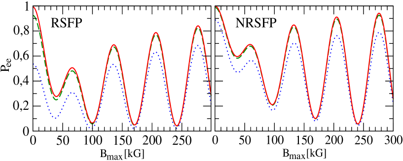
Figure 1: Neutrino survival probabilities versus magnetic field strength ($B_{\mbox{max}}$). The neutrino oscillation parameters have been fixed as $E/\Delta m^{2}=1.25\cdot 10^{8}\mbox{MeV}/\mbox{eV}^{2}$, $\tan^{2}\theta=0.001$ (solid red line), $0.01$ (green dashed line), $0.1$ (dotted blue line) in the left panel (“light” side). The corresponding numbers for the “dark”-side (right panel) are $E/\Delta m^{2}=2.5\cdot 10^{8}\mbox{MeV}/\mbox{eV}^{2}$, $\tan^{2}\theta=10$ (dotted blue line), $100$ (green dashed line), $1000$ (solid red line). Here we fix $\mu=10^{-11}$ Bohr magneton.

One can see that, both for “light” side (RSFP-like) and “dark”-side (NRSFP-like) solutions the neutrino survival probabilities exhibit an approximately periodic behavior with respect to $\mu B_{\perp}$. Note that we have fixed a transition magnetic moment of $10^{-11}$ Bohr magneton, consistent with existing present experiments. Examining Fig. 1 one sees that the smallest magnetic field magnitude which leads to a boron neutrino survival at the required level lies close to 80 KGauss. For simplicity, in what follows we will adopt such optimum strength $B_{\perp}\sim 80$ KGauss, because, being the smallest, it is probably the one preferred by astrophysics. It is straightforward to repeat our analysis for higher field strengths. This will lead to “recurrences” in solution-space, i.e. to the existence of additional branches of the RSFP-like solutions, such as can be seen, for example, from Figs. 4 and 6 in ref. Miranda:2001bi . Similarly, there will be additional branches of the “basic” NRSFP-like solution found in ref. Miranda:2001hv . For simplicity we focus, in what follows, on the analysis of the “first” RSFP and NRSFP-like solutions, and their comparison with today’s favorite oscillation solution, LMA.

In Fig. 2 we show a schematic view of the spin flavour precession survival probabilities for both resonant and non-resonant cases, RSFP (middle panel) and NRSFP (right panel). The survival probabilities for the LMA case is also shown, for comparison, in the left panel.

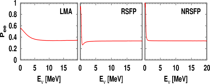
Figure 2: Optimum two-neutrino survival probabilities for the LMA (left panel) and for the two SFP solutions: RSFP (middle panel) and NRSFP (right panel).

For the LMA case the neutrinos are converted into muon neutrinos, while for the SFP scenario, the neutrinos are mainly converted into muon anti-neutrinos. Note that the above survival probabilities have been given for the best-fit parameter values determined in our fit (see table 1, below).

III Fit procedure

Global analyzes of solar neutrino data have become quite standard, for a recent reference see Maltoni:2002ni . Here we briefly describe the main features of our analysis.

In order to determine the expected event numbers for the various solar neutrino experiments we calculate the $\nu_{e}$ survival probability for each point in parameter space. We adopt Standard Solar Model neutrino fluxes BP00 , treating however the ⁸B neutrino flux normalization as a free parameter $f_{B}$, which is constrained by the SNO NC measurement. In order to determine the expected signal in each detector, these fluxes are convoluted with the survival probability at the detector, the neutrino cross-sections and the detector response functions for Super-Kamiokande Fukuda:2002pe and SNO respsno . We use the efficiencies employed previously, e. g. in ref. Maltoni:2002ni . For the SNO case the charged current and NC cross-sections of neutrinos on deuterium were taken from ref. crossno and the response functions in  respsno .

We also include theoretical and experimental errors and their cross–correlations, following the standard covariance approach. In particular, the errors associated to the energy-scale and the energy-resolution uncertainties of the Super–Kamiokande and SNO experiments are included.

Here we use all current solar neutrino data sun-exp : the solar neutrino rates of the chlorine experiment ($2.56\pm 0.16\pm 0.16$ SNU), the most recent gallium results SAGE ($70.8\leavevmode\nobreak\ ^{+5.3}_{-5.2}\leavevmode\nobreak\ {}^{+3.7}_{-3.2}$ SNU) and GALLEX/GNO ($70.8\pm 4.5\pm 3.8$ SNU), as well as the 1496-days Super-Kamiokande data sample Fukuda:2002pe in the form of 44 bins (8 energy bins, 6 of which are further divided into 7 zenith angle bins). In addition to this, we include the latest results from SNO presented in Refs. Ahmad:2002jz ; Ahmad:2002ka , in the form of 34 data bins (17 energy bins for each day and night period).

Therefore we have in total $3+44+34=81$ observables in our statistical analysis, which we fit in terms of the parameters $\Delta m^{2}{sol}$, $\theta{sol}$. The third parameter $\mu B_{\perp}$ characterizing the maximum magnitude of the magnetic field in the convective zone is fixed at its optimum value $B_{\perp}=84$ KGauss. As mentioned, we employ the self-consistent magneto-hydrodynamics magnetic field profile obtained in ref.  Miranda:2001bi for k=6 and $R_{0}=0.6R_{\odot}$.

We have compared the data described above with the expected event numbers, taking into account the relevant detector characteristics and response functions. Using a suitable definition of $\chi^{2}{sol}$ (the same as in ref. Maltoni:2002ni , except that we leave the boron flux free and remove the corresponding theoretical flux errors from the covariance matrix) we have performed a global fit of present solar neutrino data. The allowed regions for a given C.L. are defined as the set of points satisfying the condition

$$\chi^{2}_{\rm SOL}(\Delta m^{2},\theta)-\chi^{2}_{\rm SOL,min}\leq\Delta\chi^{2}\mbox{(C.L., 2\leavevmode\nobreak\ d.o.f.)},$$ (3)

where $\Delta\chi^{2}(\text{C.L. ,d.o.f.})$= 4.61, 5.99, 9.21, 11.83 for 90, 95, 99 C.L. and 3$\sigma$, respectively.

We present in Fig. 3 the allowed regions of $\tan^{2}\theta{sol}$ and $\Delta m^{2}{sol}$ for the two-flavour spin-flavor-precession.

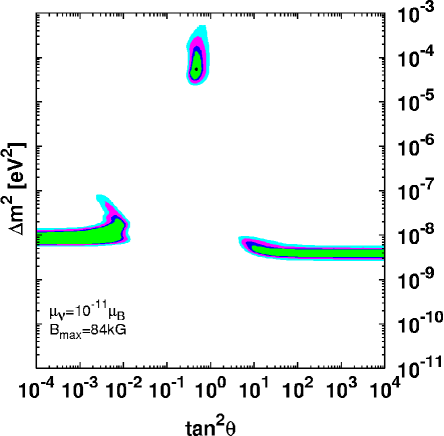
Figure 3: Allowed regions of $\tan^{2}\theta{sol}$ and $\Delta m^{2}{sol}$ for the two-flavour spin flavor precession solutions RSFP and NRSFP as well as the LMA oscillation solution.

The confidence levels are $90\%$, $95\%$, $99\%$ and $3\sigma$ for 2 d.o.f.. As noted previously, we re-confirm the appearance of two new solutions, totally due to the effect of the magnetic field. The first is the RSFP solution Miranda:2001bi , which extends up to $\tan^{2}\theta$ values around $10^{-2}$ or so. In addition, one finds a non-resonant (NRSFP) solution Miranda:2001hv in the “dark-side” of parameter space, for large $\tan^{2}\theta$ values. The fits corresponding to these two spin flavor precession solutions are slightly better than that for the LMA solution, which is recovered without any essential change due to the effect of the magnetic moment. Note, however, that the contours are defined with respect to the global minimum of $\chi^{2}$, and that this is located at the RSFP solution. As a result the LMA region in our case is slightly smaller than the one corresponding to the pure oscillation case (no magnetic field) Maltoni:2002ni  .

A characteristic feature of spin flavor precession solutions is that they produce anti-electron neutrinos, in contrast to the oscillation case. One of the new features of our present results is that, in contrast to what was found previously Miranda:2001hv ; Miranda:2001bi , the solar data alone are now sufficient to rule out all oscillation solutions other than LMA, without need to include as part of our $\chi^{2}{sol}$ the term corresponding to the data of the LSD experiment Aglietta:1996zu or the electron anti-neutrino Super-K flux limits smy . While the inclusion of these terms would reduce the two SFP branches, in this paper we will show how the solar neutrino data sample including the solar anti-neutrino rates at SNO leads to the same effect. Before we do that, let us first generalize the neutral and charged flux discussion given by SNO Ahmad:2002jz to the case where there is also a third flux, namely that of solar anti-neutrinos, expected in the SFP scenario.

In Fig. 4 we display the solar neutrinos fluxes including the electron-antineutrino flux, namely $\Phi_{\nu_{e}}$, $\Phi_{\nu_{\mu}\bar{\nu}_{\mu}}$ = $\Phi_{\nu_{\mu}}$+$\Phi_{\bar{\nu}_{\mu}}$ and $\Phi_{\bar{\nu}_{e}}$ as derived from the observed SNO event number, assuming undistorted ⁸B spectrum. Note that fluxes are in units of $10^{6}\>\mbox{cm}^{-2}\mbox{s}^{-1}$ and that here we assume the SSM boron flux prediction.

In the left panel we give the muon neutrino flux versus the electron neutrino flux. The middle and right panels we give the electron anti-neutrino flux versus electron neutrino flux (middle) and versus the muon-type neutrino flux (right). These contours correspond to 68 % C.L. and $90\%$ C.L. for 2 d.o.f.. One sees that the electron anti-neutrino flux, calculated with the cross sections in crossno , is constrained in model-independent way to be less than $1\cdot 10^{6}\mbox{cm}^{-2}\mbox{s}^{-1}$ at 90 % C.L. The best fitted fluxes are: $\Phi_{\nu_{e}}=1.79\cdot 10^{6}\>\mbox{cm}^{-2}\mbox{s}^{-1}$, $\Phi_{\nu_{\mu}\bar{\nu}_{\mu}}=3.02\cdot 10^{6}\>\mbox{cm}^{-2}\mbox{s}^{-1}$, $\Phi_{\bar{\nu}_{e}}=0.14\cdot 10^{6}\>\mbox{cm}^{-2}\mbox{s}^{-1}$, with $\chi^{2}_{\mbox{min}}=16.7$ and 15 d.o.f.. Note that the best fit flux $\Phi_{\bar{\nu}_{e}}$ shown by stars in Fig. 4 is compatible with zero at $97\%$ C.L.

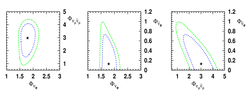
Figure 4: Solar neutrinos fluxes $\Phi_{\nu_{e}}$, $\Phi_{\nu_{\mu}\bar{\nu}_{\mu}}$=$\Phi_{\nu_{\mu}}$+$\Phi_{\bar{\nu}_{\mu}}$ and $\Phi_{\bar{\nu}_{e}}$ (in units of $10^{6}\>\mbox{cm}^{-2}\mbox{s}^{-1}$) derived from the number of events per bin at SNO for undistorted ⁸B spectrum.

Encouraged by the consistency of our generalization of the SNO procedure for the SFP case, we now move to the inclusion of the anti-neutrino data in the analysis. The reaction $\bar{\nu_{e}}+D\to n+n+e^{+}$ would lead, in addition to the positron Cerenkov light, to the capture of 2 neutrons by deuteron(s) and the production of two mono-chromatic gammas with energy $E_{\gamma}\approx$ 6.25 MeV. Clearly a complete analysis of the associated signal arising from this can not be performed at the moment, since we lack the appropriate response function . As an approximation we can, however, assume that the positron resolution function is the same as for electrons, and also that the two neutrons can be captured by Deuterum in the same way as the neutrons in the NC channel (this last contribution is the most important one). Under this approximation we obtain in Fig. 5 an estimate of the allowed regions. Particularly noticeable is the fact that in this case the dark side region becomes smaller. This cut is required in order to avoid an unacceptably high solar anti-neutrino flux (above 20 % or so of the boron-8 neutrino flux) for values of $\tan^{2}\theta\mathrel{\hbox to0.0pt{\lower 4.0pt\hbox{\hskip 1.0pt$\sim$}\hss}\raise 1.0pt\hbox{$<$}}20$. This exercise highlights the relevance of solar anti-neutrino searches at SNO in restricting the parameter space of SFP solutions. Such possibility using Super-K is certainly less favorable.

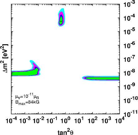
Figure 5: Same plot as in Fig. 3, but including electron antineutrino CC interaction in SNO ($\bar{\nu_{e}}+D\to n+n+e^{+}$) with the approximation discussed in text.

Before we conclude this section let us present in table 1 the goodness-of-fit (GOF) corresponding to each of our three solutions. The analysis has been done for 81 (Chlorine + GNO + SAGE + Zenith SK spectrum + SNO D/N Spectrum) - 3 parameters: $\tan^{2}\theta{sol}$, $\Delta m^{2}{sol}$, and the boron flux $f_{B}$, corresponding to 78 d.o.f. This table shows the best-fit parameter values, $\chi^{2}_{\mbox{min}}$ and GOF for the three solutions. The top panel refers to the usual oscillation case, the middle panel corresponds to the fit without including the SNO anti-neutrino CC interaction and the bottom panel is for the case where this interaction is included.

Region	$\tan^{2}\theta$	$\Delta m^{2}$	$\chi^{2}_{\mbox{min}}$	g.o.f.
standard oscillation
LMA	$0.47$	$5.6\cdot 10^{-5}$	68.0	78%
$\mu_{\nu}B\neq 0$ without SNO CC $\bar{\nu}_{e}$
RSFP	$4.2\cdot 10^{-4}$	$7.9\cdot 10^{-9}$	66.1	83%
NRSFP	$119$	$4.0\cdot 10^{-9}$	66.4	82%
LMA	$0.47$	$5.6\cdot 10^{-5}$	68.0	78%
$\mu_{\nu}B\neq 0$ with SNO CC $\bar{\nu}_{e}$
RSFP	$5.3\cdot 10^{-4}$	$7.9\cdot 10^{-9}$	65.8	84%
NRSFP	$3\cdot 10^{3}$	$4.0\cdot 10^{-9}$	66.4	82%
LMA	$0.47$	$5.6\cdot 10^{-5}$	68.1	78%

Table 1: Best fit values of $\Delta m^{2}$ and $\tan^{2}\theta$ with the corresponding $\chi^{2}_{\mbox{min}}$ and GOF for the standard oscillation case (top panel) and for non-zero magnetic field (middle and bottom panels). The squared mass differences are given in eV².

To close this session we now illustrate more concisely the above results by displaying in Fig. 6 the profiles of $\Delta\chi^{2}{sol}$ as a function of $\tan^{2}\theta{sol}$. This is obtained by minimizing with respect to the undisplayed oscillation parameters, for the fixed $\mu B_{\perp}$ value indicated above.

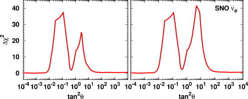
Figure 6: $\Delta\chi^{2}{sol}$ as a function of $\tan^{2}\theta$ with respect to the favored spin-flavor-precession solution

Note that the $\Delta\chi^{2}{sol}$ is calculated with respect to the favored spin-flavor-precession solution. The first thing to notice are the two plateaus corresponding to the RSFP and NRSFP solutions, slightly lower than the LMA $\chi^{2}_{\mbox{min}}$. In contrast to the left panel, the right panel includes the electron anti-neutrino CC interaction in SNO. One can see how the NRSFP plateau has now become narrower (see also Fig. 5). Moreover one can appreciate two very small kinks corresponding to the “would-be” LOW solutions. Their status worsens and their position shifts slightly towards the “dark side”.

IV Future Experiments

We have seen how the SFP scenario leads to three very good descriptions of current solar neutrino data corresponding to the RSFP, NSRFP and the LMA solutions. The issue comes as to how to distinguish between these solutions, which are presently statistically equivalent. Note that this is not such an easy task since, as seen in Fig. 2, the expected spectral energy distribution for our spin flavour precession solutions is hardly distinguishable from the one expected in the pure LMA oscillation solution. Moreover, in contrast to the oscillation solution, where a day-night effect is predicted, the SFP spectra show no day-night asymmetry.

There is at the moment great expectation as to the first physics results of the upcoming KamLAND experiment, expected shortly kamland . Here we analyse the implications of two possible outcomes of the KamLAND experiment for the status of SFP solutions.

IV.1 If KamLAND confirms the LMA oscillation solution

In this case all alternative solutions, such as the present spin-flavor-precession solutions, may be present only at a sub-leading level and, on the basis of how good is the KamLAND determination of the LMA oscillation parameters, one will correspondingly constrain any exotic alternative. Our resulting constraints on the SFP solutions are illustrated in Fig. 7.

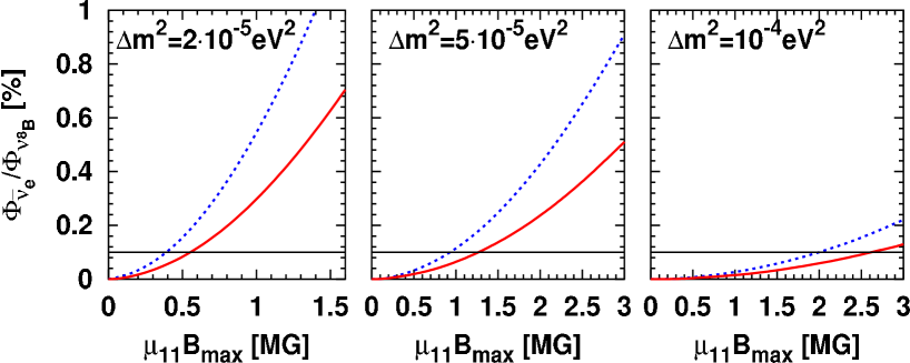
Figure 7: KamLAND sensitivity on the Majorana neutrino transition magnetic moment in case the LMA solution is confirmed. See text.

In Fig. 7 we have displayed the electron anti-neutrino flux predicted at KamLAND ($E>8.3$ MeV) for three different $\Delta m^{2}{sol}$ values (indicated in the figure) and for $\tan^{2}\theta{sol}$ values varying in the range from 0.3-0.8, as a function of $\mu_{11}B_{\text{m}ax}$, $\mu_{11}$ being the magnetic moment in units of $10^{-11}$ Bohr magneton and $B_{\text{m}ax}$ being the maximum magnetic field in the convective zone. In order to obtain such a simple correlation we note the importance of using our self-consistent magneto-hydrodynamics magnetic field profile, as in ref.  Miranda:2001bi . The extremes of the neutrino mixing range correspond to the solid and dashed lines indicated in the figure, while the horizontal line corresponds to a KamLAND sensitivity on the anti-neutrino flux of 0.1 %, expected with three years running kamland . Clearly the limits on the transition magnetic moments are sensitive also to the ultimate central $\Delta m^{2}{sol}$ value indicated by KamLAND (a 10 % error is expected), being more stringent for lower $\Delta m^{2}{sol}$ values, as seen from the left panel.

IV.2 If KamLAND does not confirm the LMA solution

Imagine now the extreme and unlikely case that KamLAND does not provide useful information on the neutrino parameters. In this case one can compare the predictions of these three solutions for the upcoming Borexino experiment, as suggested in ref. Akhmedov:2002ti .

A simple way to display this is presented in Fig. 8. This figure shows the predicted values for

$$R_{\rm Borexino}\equiv\frac{\rm observed\>Borexino\>rate}{\rm SSM\>rate}$$ (4)

defined as the ratio of observed-over-SSM-expected signal in Borexino, assuming best-fit parameters as determined in our fit, and 90%C.L. error bars for LMA (left line), RSFP (middle lines) and NRSFP (right lines) solutions. For the SFP solutions two error bars are indicated for $R_{\rm Borexino}$.

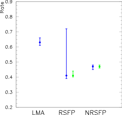
Figure 8: Predicted $R_{\rm Borexino}$ values for LMA and spin flavor precession solutions.

The error bars indicated in grey (green in color printers) refers to the cases $\theta=0$ for the RSFP case and $\theta=\pi/2$ for the NRSFP solution. The error bars indicated in dark (blue in color printers) correpond to the general SFP case with non-zero mixing. Clearly, the zero mixing RSFP and the LMA solutions lead to very different predictions, as already noted in ref. Akhmedov:2002ti . However, we remark that in general the RSFP solution can not be distinguished from LMA insofar as the Borexino predition is concerned. Indeed, as seen from Fig. 6, RSFP is characterized by a very flat plateau of nearly constant $\chi^{2}$, while the Borexino prediction depends rather strongly on the poorly determined value of the “best” neutrino mixing angle for this solution. To see this let us take, for example $\Delta m^{2}{sol}\sim 2\times 10^{-8}$ eV² and $\tan^{2}\theta{sol}\sim 10^{-2}$ and display the neutrino survival probability versus energy, as seen in Fig. 9.

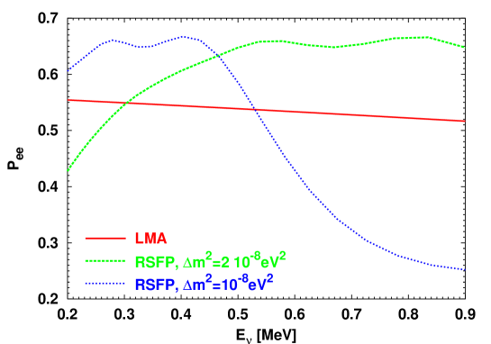
Figure 9: Neutrino survival probability for RSFP-like solution with $\Delta m^{2}{sol}\sim 2\times 10^{-8}$ eV² and $\tan^{2}\theta{sol}\sim 10^{-2}$, in the range between 0.2 and 0.9 MeV.

One sees from this figure how in the pp region this solution is similar to LMA, but leads to a much smaller suppression of the berilium line. This allows us to understand the inability to predict with precision the borexino rate expected in this part of the (lowest) RSFP region. In contrast, the NRSFP solution in the “dark-side” is the one which is more clearly distinguishable from the LMA oscillation solution. Moreover, we have verified that, for the case of the NRSFP solution the Borexino predition is rather insensitive to whether the neutrino mixing is left free or not.

A more complete way to present this information is displayed in Fig. 10. Here we have overlapped the allowed neutrino parameter ranges determined from our fit with the predicted $R_{\rm Borexino}$ values, for each one of these solutions, RSFP, NRSFP and LMA at 90%C.L. The results for the LMA solution agree well with those obtained, say, in refs. Bahcall:2002hv ; deHolanda:2002pp . We can clearly identify from Fig. 10 which range in the 90 % allowed confidence RSFP region leads to the large “spread” in the borexino prediction discussed previously.

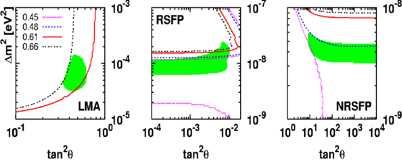
Figure 10: Contour lines of predicted $R_{\rm Borexino}$ values as a function of the neutrino oscillation parameters. The shaded regions correspond to the three solutions discussed here (LMA, left panel), RSFP (middel panel) and NRSFP (right panel). See text.

V Summary and Discussion

In this paper we have re-considered the solutions of the solar neutrino problem involving two-flavor oscillations and spin-flavour precessions. We have given a global analysis of such SFP solutions to the solar neutrino problem, taking into account the impact of the full set of latest solar neutrino data, including the recent SNO data as well as the 1496–day Super-Kamiokande data. These are characterized by three effective parameters: $\Delta m^{2}{sol}\equiv\Delta m^{2}$, the neutrino mixing angle $\theta{sol}\equiv\theta$ and the magnetic field parameter $\mu B_{\perp}$. For the latter we have fixed $\mu=10^{-11}$ Bohr magneton, with a corresponding optimized self-consistent magneto-hydrodynamics magnetic field profile with $B_{\perp}\sim 80$ KGauss as the maximum field strength in the convective zone. Two-flavor oscillations are recovered as a particular case of our general SFP scenario. We have found that no LOW-quasi-vacuum or vacuum solutions are present at the 3 $\sigma$ level. In addition to the standard LMA oscillation solution, we have re-confirmed the existence of two SFP solutions, in the resonant (RSFP) and non-resonant (NRSFP) regimes. These two SFP solutions have goodness of fit 84 % (RSFP) and 83 % (NRSFP), slightly better than the LMA oscillation solution (78 %). We have discussed the role of solar anti-neutrino searches in the fit and present a table of best-fit parameters and $\chi^{2}_{\text{min}}$ values. Should KamLAND confirm the LMA solution, the SFP solutions may at best be present at a sub-leading level, leading to a meaningful constraint on $\mu B_{\perp}$. If the magnetic field strength is known from solar physics, we can obtain a bound on the Majorana neutrino transition magnetic moment, complementary to the bounds discussed in ref. gri02 . In the event LMA is not the solution realized in nature, then future experiments such as Borexino can be of help in distinguishing LMA from the NRSFP solution, as well as the restricted RSFP solution with no mixing.

Appendix A Implication of the KamLAND results

The original version of this paper indicated that both RSFP and NRSFP descriptions of the solar neutrino data were slightly better than the favoured LMA-MSW solution. Since then the results of the first 145.1 days of reactor neutrino observations at the KamLAND experiment have been published Eguchi:2002dm . Complementing our discussion in Section IV here we analyze the implications of KamLAND results for the neutrino spin-flavor precession hypothsis.

KamLAND is a reactor neutrino experiment whose detector is located at the Kamiokande site. Most of the $\overline{\nu}_{e}$ flux incident at KamLAND comes from nuclear plants at distances 80-350 km from the detector, making the average baseline of about 180 km, long enough to test the LMA-MSW region. The target for the $\overline{\nu}_{e}$ flux consists of a spherical transparent balloon filled with 1000 tons of non-doped liquid scintillator, and the antineutrinos are detected via the inverse neutron $\beta$-decay process $\overline{\nu}_{e}+p\to e^{+}+n$. The KamLAND collaboration has for the first time observed the disappearance of neutrinos produced in a power reactor during their flight over such distances. The ratio of the observed events to the expected number is $0.611\pm 0.085{\rm(stat)}\pm 0.041{\rm(syst)}$ for $\bar{\nu}_{e}$ energies $>$ 3.4 MeV. This gives the first terrestrial confirmation of the solar neutrino anomaly and also confirms the oscillation hypothesis with man-produced neutrinos.

The global analysis of solar+KamLAND data for pure neutrino oscillations (neglecting possible sub-leading effects such as spin-flavor precession) has been given in Maltoni:2002aw . Assuming CPT invariance the main result is that all other flavor oscillation solutions such as vacuum oscillations, SMA-MSW and LOW are in disagreement with KamLAND data at more than 99.73 % C. L. We expect that, under the same CPT invariance assumption, all non-oscillation solutions will also be rejected, as these would not account for the reduced reactor neutrino flux detected at KamLAND. In fact this has already been shown for Non-Standard neutrino matter Interaction hypothesis (NSI) Guzzo:2001mi .

We have used the Poisson distribution in the analysis of the KamLAND data, adding this to our previous result for the solar data. Besides our previous Boron free analysis, we have also made a Boron fixed analysis.

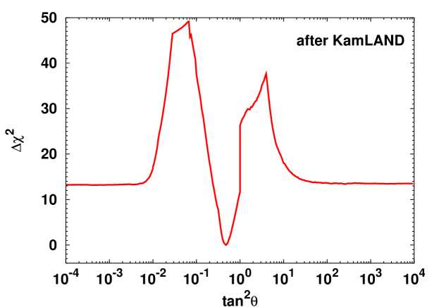
Figure 11: $\Delta\chi^{2}_{\mathsc{sol}+KamLAND}$ as a function of $\tan^{2}\theta$ with respect to the favored LMA solution

We find that, after adding the KamLAND result, the RSFP and NRSFP solutions are allowed only at 99.86 % C. L. and 99.88 % C. L., respectively. Thus the spin flavor precession solution to the solar neutrino problem can not be reconciled with the KamLAND data and is therefore rejected. In Fig. 11 the profile of $\Delta\chi^{2}_{\mathsc{sol}+KamLAND}$ as a function of $\tan^{2}\theta{sol}$ is shown. One can see how after KamLAND the RSFP and NRSFP solutions have now become disfavored in contrast to Fig. 6 for the solar data only. Spin-flavor precessions may however be present at a subleading level. Future data may be used to place limits on neutrino magnetic moments and solar magnetic fields. In particular, for strong solar magnetic fields and large enough neutrino transition magnetic moment the LMA-MSW allowed region may be potentially distorted.