Baryon Form Factors at High Momentum Transfer and GPD’s

Abstract

Nucleon elastic and transition form factors at high momentum transfer $-t$ are treated in terms of generalized parton distributions in a two-body framework. In this framework the high $-t$ dependence of the form factors give information about the high $k_{\perp}$ , or short distance $b_{\perp}$ correlations of nucleon model wave functions. Applications are made to elastic and resonance nucleon form factors, and real Compton Scattering.

During the past several years there has been considerable discussion of how to describe exclusive reactions at momentum transfers which are experimentally attainable. While pQCD is an interesting mechanism which probes the simplest Fock state component of the hadron, most theoretical studies agree that even at the highest attainable momentum transfers, there is a large soft contribution which involves more complex components of the hadronic wave functions. The so-called handbag [1] mechanism has evolved to describe such soft processes, and achieves its full power at high momentum transfer where a process can be factorized into a fully perturbative hard amplitude and a generalized parton distribution (GPD) [2] [3] [4], which represents the off-diagonal probability of the interacting quark being placed back into the remaining hadron, keeping it in-tact at a different transfered longitudinal momentum. The power of the mechanism is that the same soft GPD, which contains the information about the hadronic structure is accessed in a variety of different reactions, while the hard perturbative part is reaction specific. The GPD’s give us unique information about the longitudinal ($x$) and transverse ($k_{\perp}$) parton momentum distributions, and importantly, about the interference between the initial parton wave function and the phase shifted final parton wave function.

The GPD approach manifests itself in two kinematical regimes, corresponding to the $t$ dependent form factor type reaction, and the $t\to t_{min}$ off-forward production of mesons or photons. Here we focus on the former. In such a reaction the incident real or virtual photon interacts perturbatively with one of the quarks within the hadron, which is re-absorbed into the hadron leaving it in-tact or in a higher resonant state. This is a Feynman type reaction which involves the full complexity of the non-perturbative nucleon structure, as opposed to the leading order pQCD mechanism, which involves only the valence quark Fock state. Form factors are the $x$ moments of the GPD’s, and as such constrain the longitudinal dependence of the nucleon structure. As a function of $t$ they uniquely constrain the $k_{\perp}$ dependence of the nucleon’s wave functions. Fourier transforms of the GPD’s - $\mathcal{F}_{b}(x,\vec{b}_{\perp})\propto\int\vec{dq}_{\perp}exp(i\vec{b}_{\perp}\cdot\vec{q}_{\perp})\mathcal{F}(x,t)$ -, directly give the transverse spatial impact parameter distribution of the quarks for each longitudinal momentum fraction [5]. Thus, together with $x$ distributions obtained in DIS the $k_{\perp}$ accessed in form factor measurements give us a unique 3 dimensional picture of the quark distributions in the nucleon. Examples of reactions accessible via GPDs include the nucleon elastic Dirac and Pauli form factors $F_{1}$ and $F_{2}$ (or equivalently $G_{Ep}$ and $G_{Mp}$), resonance transition amplitudes such as $A_{1/2}$ for $N\to S_{11}(1535)$, or $G_{M}^{*}$ for $N\to\Delta$, and Compton scattering form factors $R_{V}$ and $R_{A}$ and their polarization asymmetries. The relationship of the GPD’s to these various form factors is given as follows:

For elastic scattering

$$F_{1}(t)=\int^{1}_{0}\sum_{q}\mathcal{F}^{q}(x,t)dx\hskip 21.68121ptF_{2}(t)=\int^{1}_{0}\sum_{q}\mathcal{K}^{q}(x,t)dx.$$ (1)

where $q$ signifies both quark and anti-quark flavors. We work in a reference frame in which the total momentum transfer is transverse so that $\zeta$=0, and denote $\mathcal{F}^{q}(x,t)\equiv\mathcal{F}^{q}_{0}(x,t)$,  $\mathcal{K}^{q}(x,t)\equiv\mathcal{K}^{q}_{0}(x,t)$.

For Compton scattering [6]

$$R_{1}(t)=\int^{1}_{0}\sum_{q}{1\over x}\mathcal{F}^{q}(x,t)dx\hskip 21.68121ptR_{2}(t)=\int^{1}_{0}\sum_{q}{1\over x}\mathcal{K}^{q}(x,t)dx.$$ (2)

Resonance transition form factors access components of the GPD’s which are not accessed in elastic scattering or Compton scattering. The $N\to\Delta$ form factors are related to isovector components of the GPD’s [7] [8].

$$G^{*}_{M}=\int^{1}_{0}\sum_{q}\mathcal{F}^{q}_{M}(x,t)dx\ \ \ G^{*}_{E}=\int^{1}_{0}\sum_{q}\mathcal{F}^{q}_{E}(x,t)dx\ \ \ G^{*}_{C}=\int^{1}_{0}\sum_{q}\mathcal{F}^{q}_{C}(x,t)dx$$ (3)

where $G^{*}_{M}$, $G^{*}_{E}$ and $G^{*}_{C}$ are magnetic, electric and Coulomb transition form factors [9], and $\mathcal{F}^{q}_{M}$, $\mathcal{F}^{q}_{E}$, and $\mathcal{F}^{q}_{C}$ are axial (isovector) GPD’s, which can be related to elastic GPD’s in the large $N_{C}$ limit through isospin rotations [8]. The $N\to S_{11}$ transition form factor is also important, as it probes fundamental aspects of dynamical chiral symmetry breaking in QCD. If chiral symmetry were not broken, the $S_{11}$ would be the nucleon’s parity partner and the $N$ and $S_{11}$ masses would be degenerate.

As a basis for constructing the GPD’s we use the two-body model introduced in [6] whose connection with the handbag is illustrated in fig. 1.

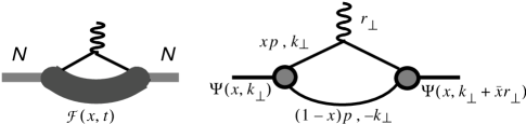
Figure 1: Schematic relation between the two-body and handbag mechanisms discussed in the text.

In this framework the GPD is written

$$\mathcal{F}(x,t)=\int{\Psi^{*}(x,k_{\perp}+\bar{x}r_{\perp})\Psi(x,k_{\perp}){{d^{2}k_{\perp}}\over{16\pi^{3}}}}$$ (4)

where $\bar{x}\equiv 1-x$,

An example of a specific model wave function [10] is

$$\Psi(x,k_{\perp})=\Phi(x)\left(A_{s}e^{-k_{\perp}^{2}/2x\bar{x}\lambda^{2}}+A_{h}{{x\bar{x}\Lambda^{2}}\over{k_{\perp}^{2}+\Lambda^{2}}}\right)\equiv\Psi_{soft}+\Psi_{hard}\\$$ (5)

The function $\Phi(x)$ is constrained so that $\mathcal{F}(x,0)$ reduces to the valence quark distribution $f(x)$. It was shown in ref. [10] that although a Gaussian form of the $k_{\perp}$ dependence in $\Psi_{soft}$ accounts for the magnitude and shape of the elastic $F_{1}$ for $Q^{2}$ below several GeV², it is inadequate at higher $Q^{2}$. However, the addition of a small $\Psi_{hard}$ component in eq. (5) can dramatically improve the agreement at high $Q^{2}$. As an example of a power law dependence, we choose an ad-hoc $1/k_{\perp}^{2}$ behavior with lower cutoff parameter $\Lambda$. A similar parameterization is chosen for $F_{2}$ with $\mathcal{K}^{q}(x,0)=\sqrt{(1-x)}\mathcal{F}^{q}(x,0)$. In order to constrain the parameters of eq. (5) the available data on both $G_{Mp}$ and $G_{Ep}/G_{Mp}$ were simultaneously reproduced, giving $A_{s}=\sqrt{1-A_{h}^{2}}=0.97$, $A_{H}=0.24$, $\lambda_{1}^{2}=0.6$ GeV² and $\lambda_{2}^{2}=0.45$ GeV². The function $\Psi(k_{\perp})=\int{\Psi(k_{\perp},x)dx}$ is shown in fig. 2. Only at $k_{\perp}$ greater than about 1 GeV does the hard tail important.

The fits to the data using respectively $\Psi=\Psi_{soft}+\Psi_{hard}$, and $\Psi=\Psi_{soft}$ are shown in figs. 3 4 6.

Figure 2: The function $\Psi(k_{\perp})\equiv\int{\Psi(x,k_{\perp})dx}$ vs. $k_{\perp}$. The dashed curve is due to the soft Gaussian component $\Psi_{soft}$, with $\lambda^{2}=0.6\ {\rm GeV^{2}}$. The solid curve is $\Psi_{soft}+\Psi_{hard}$, with $A_{h}$ = 0.24, $k_{\perp,max}$ = 4 GeV, and cutoff parameter $\Lambda$ = 0.45 GeV.

file=wf.epsi,angle=90,width=2.4in

As seen in the top panel of fig. 3, this rather small addition of high momentum components can account for the high, as well as the low $Q^{2}$ magnetic form factor. Interestingly, ref. [11]found that even in a pQCD calculation a power law tail is useful in reproducing the high $Q^{2}$ data.

Figure 3: Upper: Proton magnetic form factor $G_{Mp}/G_{D}$, where $G_{D}=1/(1+Q^{2}/0.71)^{2}$. Data are from SLAC^9,10 with low energy data reevaluated¹¹. The dashed curve uses only $\Psi_{soft}$, while the solid curve uses $\Psi_{soft}+\Psi_{hard}$. Lower: The impact parameter dependence of the curves in the upper figure, $G_{Mp}(b_{\perp})=\int dx\mathcal{F}_{b}(x,b_{\perp})$. The curve at the bottom left labelled “hard tail” is the difference between the solid and dashed curves, which is responsible for most of the form factor at high $Q^{2}$.

file=GMp_tot_qb.epsi,angle=90,width=3in

Taking the Fourier transforms of the GPD’s gives the spatial impact parameter distribution of the struck quarks. The bottom panel in fig. 3 shows

$$\mathcal{F}_{b}(x,b_{\perp})=\int dq_{\perp}e^{i\vec{b}_{\perp}\cdot\vec{q}_{\perp}}\mathcal{F}(x,t).$$

and the effect of $\Psi_{hard}$. Only a small addition of small impact parameter components to the wave function accounts for most of the form factor at high $Q^{2}$.

In fig. 4 the obtained values of $GE_{p}/GM_{p}$ for $\Psi_{soft}+\Psi_{hard}$ and $\Psi_{hard}$ alone are compared with the recent JLab data [15].

Figure 4: $GE_{p}/GM_{p}$ for $\Psi_{soft}+\Psi_{hard}$ and $\Psi_{hard}$ alone are compared with the recent JLab data¹². The curves are as in fig. 3.

file=gegmp.epsi,angle=90,width=3in

The obtained GPD’s as a function of $x$ and $t$ are shown in fig. 5.

file=F.epsi,width=1.7in

file=K.epsi,width=1.7in

Figure 5: GPD’s as a function of $\tilde{x}$ for various values of $t$, where $\tilde{x}=x$ (x-tilde) for valence quarks, and $\tilde{x}=-x$ for the sea quarks. The figures on the left and right are for $\mathcal{F}$ and $\mathcal{K}$ respectively. The graphs for positive $\tilde{x}$ represent the valence quark contribution, while the graphs for negative $\tilde{x}$ represent the sea quark contributions. The individual curves range from $|t|$ $\sim 0$ GeV² (highest curve in each panel) to $|t|$ = 35 GeV² (lowest curve in each panel). The upper and middle panels are the GPD’s for the full wave function $\Psi_{soft}+\Psi{hard}$, while those in the lowest panels are obtained using the $\Psi_{soft}$ soft only. Note that the addition of the $\Psi_{hard}$ mainly affects the GPD’s at higher $|t|$ and $\tilde{x}<0.5$

One may apply the constraints of the elastic form factors to investigate properties of inelastic resonance transitions. For example, in the large $N_{c}$ limit the GPDs for the $N\to\Delta(1232)$ transition are expected to be isovector components of the elastic GPD, which is approximately given by

$$\mathcal{F}^{(IV)}_{M}={2\over{\sqrt{3}}}\mathcal{K}^{(IV)}_{M}={2\over{\sqrt{3}}}\left(\mathcal{K}^{u}-\mathcal{K}^{d}\right),$$

where $\mathcal{K}^{u}$ and $\mathcal{K}^{d}$ are the GPD’s for the up and down quarks respectively. Figure 6 shows the result of applying the GPD’s from elastic scattering to the $N\to\Delta$ transition. The data was renormalized by the ratio 3/2.14, to bring into line the nucleon isovector form factor at $Q^{2}$=0 with the experimental value for the $N\to\Delta$.

Figure 6: The $N\to\Delta$ magnetic form factor $G_{M}^{*}(Q^{2})$ relative to the dipole $G_{D}=3/(1+Q^{2}/.71)^{2}$

file=GMDELTA.epsi,angle=90,width=3in

In summary, it is seen that complete knowledge of the various types of baryon form factors provides very strong constraints for model wave functions and GPD’s.

References

[1]A.V. Efremov and A.V. Radyushkin, Theor. Math. Phys.42, 97 (1980)