The Off-diagonal Goldberger-Treiman Relation and Its Discrepancy

Abstract

We study the off-diagonal Goldberger-Treiman relation (ODGTR) and its discrepancy (ODGTD) in the $N$, $\Delta$, $\pi$ sector through ${\cal O}(p^{2})$ using heavy baryon chiral perturbation theory. To this order, the ODGTD and axial vector $N$ to $\Delta$ transition radius are determined solely by low energy constants. Loop corrections appear at ${\cal O}(p^{4})$. For low-energy constants of natural size, the ODGTD would represent a $\sim 2\%$ correction to the ODGTR. We discuss the implications of the ODGTR and ODGTD for lattice and quark model calculations of the transition form factors and for parity-violating electroexcitation of the $\Delta$.

PACS Indices: 11.30.Rd, 13.75.Gx

I Introduction

The Goldberger-Treiman relation (GTR) [1] plays an important role in theoretical hadronic and nuclear physics. It relates hadronic matrix elements of the weak axial current (the nucleon axial charge, $g_{A}$, and the pion decay constant, $F_{\pi}$) to quantities governed by the strong interaction (the pion nucleon strong coupling constant, $g_{\pi NN}$, and nucleon mass, $m_{N}$):

$$g_{\pi NN}={g_{A}m_{N}\over F_{\pi}}$$ (1)

The GTR represents an approximation, since $g_{\pi NN}$ is determined experimentally at the point $q^{2}=m_{\pi}^{2}$ while $g_{A}$ is measured close to the point $q^{2}=0$. In the chiral limit, the GTR would be exact, while in the physical world, it holds to an astonishing level of accuracy. The small difference between the physical value of $g_{\pi NN}$ and RHS of Eq. (1) when physical values of $g_{A}$, $F_{\pi}$ and $m_{N}$ are used is called the Goldberger-Treiman discrepancy (GTD). Physically, the GTD is driven by the explicit chiral symmetry breaking introduced by the non-zero current quark mass.

Many theoretical discussions of this chiral symmetry-breaking effect have appeared in the literature [2, 3, 4, 5, 6]. Recently the GTD in the context of SU(3$)_{L}\times$SU(3$)_{R}$ chiral symmetry has been analyzed by Goity et al. [7] within the framework of heavy baryon chiral perturbation theory (HB$\chi$PT) [8, 9]. These authors found that chiral loop corrections appear at ${\cal O}(p^{4})$. The dominant contribution comes from the low energy counterterm appearing in the ${\cal O}(p^{3})$ Lagrangian. Their result is consistent with more conventional approaches where current quark mass plays an explicit role [2, 3].

In this work we analyze the off-diagonal Goldberger-Treiman relation (ODGTR) and its discrepancy for the $SU(2)$ $\pi$, $N$, $\Delta$ sector. As we show below, both the magnitude of, and theoretical uncertainty in, the off-diagonal Goldberger-Treiman discrepancy (ODGTD) is $\sim m_{\pi}^{2}/\Lambda_{\chi}^{2}\sim 0.01$, where $\Lambda_{\chi}=4\pi F_{\pi}\sim 1$ GeV is the scale of chiral symmetry breaking. Consequently, the ODGTR provides a useful benchmark for both experimental and theoretical studies of the axial vector $N\to\Delta$ transition form factors. In principle, the ODGTR can be tested using charged current reactions, such as neutrino excitation of the $\Delta$, or weak neutral current processes, such as parity-violating (PV) electroexcitation. These processes are sensitive to axial vector transition form factors, which can be related to the strong $\pi N\Delta$ coupling via the ODGTR. The values for these form factors obtained from charged current scattering are fairly uncertain. A measurement of the PV asymmetry for neutral current electroexcitation will be performed at the Jefferson Lab by the G0 Collaboration[10] in hopes of providing a more precise determination of the axial transition form factors. The ODGTR also provides a check on lattice QCD and hadron model calculations of the axial transition form factors. From either perspective, the theoretical analysis of the ODGTR using HB$\chi$PT appears to be a timely endeavor.

II Notations

We follow the standard HB$\chi$PT formalism [8, 9] and introduce the following notations:

$$\Sigma=\xi^{2}\ ,\ \ \xi=e^{i\pi\over F_{\pi}}\ ,\ \ \pi={1\over 2}\pi^{a}\tau^{a}$$ (2)

with $F_{\pi}=92.4$ MeV being the pion decay constant. The chiral vector and axial vector currents are given by

$${\cal D}_{\mu} = D_{\mu}+V_{\mu}$$ (3)

$$A_{\mu} = {i\over 2}\xi^{\dagger}(D_{\mu}\Sigma)\xi^{\dagger}$$ (4)

$$V_{\mu} = {1\over 2}(\xi\partial_{\mu}\xi^{\dagger}+\xi^{\dagger}\partial_{\mu}\xi)-{i\over 2}\xi^{\dagger}r_{\mu}\xi-{i\over 2}\xi l_{\mu}\xi^{\dagger}$$ (5)

$$D_{\mu}\Sigma = \partial_{\mu}\Sigma-ir_{\mu}\Sigma+i\Sigma l_{\mu}$$ (6)

$$r_{\mu} = {\tilde{v}}_{\mu}+a_{\mu}$$ (7)

$$l_{\mu} = {\tilde{v}}_{\mu}-a_{\mu}$$ (8)

$$F_{R}^{\mu\nu} = \partial^{\mu}r^{\nu}-\partial^{\nu}r^{\mu}-i[r^{\mu},r^{\nu}]$$ (9)

$$F_{L}^{\mu\nu} = \partial^{\mu}l^{\nu}-\partial^{\nu}l^{\mu}-i[l^{\mu},l^{\nu}]$$ (10)

$$f_{\pm}^{\mu\nu} = \xi F_{L}^{\mu\nu}\xi^{\dagger}\pm\xi^{\dagger}F_{R}^{\mu\nu}\xi$$ (11)

$$\chi = 2B_{0}(s+ip)$$ (12)

$$\chi_{\pm} = \xi^{\dagger}\chi\xi^{\dagger}\pm\xi\chi^{\dagger}\xi\ \ \ ,$$ (13)

where $s,p,a_{\mu},{\tilde{v}}_{\mu}$ are the scalar, pseudoscalar, pseudovector, and vector external sources with $p=p^{i}\tau^{i}$ and $a_{\mu}=a_{\mu}^{i}{\tau^{i}\over 2}$.

For the $\Delta$, we use the isospurion formalism, treating the $\Delta$ field $T_{\mu}^{i}(x)$ as a vector spinor in both spin and isospin space [11] with the constraint $\tau^{i}T_{\mu}^{i}(x)=0$. The components of this field are

$$T^{3}_{\mu}=-\sqrt{{2\over 3}}\left(\begin{array}[]{l}\Delta^{+}\\ \Delta^{0}\end{array}\right)_{\mu},$$ (16)

$$T^{+}_{\mu}=\left(\begin{array}[]{l}\Delta^{++}\\ \Delta^{+}/\sqrt{3}\end{array}\right)_{\mu},$$ (19)

$$T^{-}_{\mu}=-\left(\begin{array}[]{l}\Delta^{0}/\sqrt{3}\\ \Delta^{-}\end{array}\right)_{\mu}.$$ (22)

The field $T^{i}_{\mu}$ also satisfies the constraints for the ordinary Schwinger-Rarita spin-${3\over 2}$ field,

$$\gamma^{\mu}T_{\mu}^{i}=0\ \ \ {\hbox{and}}\ \ \ p^{\mu}T_{\mu}^{i}=0\ \ \ .$$ (23)

We eventually convert to the heavy baryon expansion, in which case the latter constraint becomes $v^{\mu}T_{\mu}^{i}=0$ with $v_{\mu}$ being the heavy baryon velocity.

In order to obtain proper chiral counting for the nucleon, we employ the conventional heavy baryon expansion, and in order to consistently include the $\Delta$ we follow the small scale expansion developed in [11]. In this approach external energy and momenta, the $\Delta$ and nucleon mass difference $\delta\equiv m_{\Delta}-m_{N}$ and $1/m_{N}$ are all treated as ${\cal O}(\epsilon)$ in chiral power counting.

The leading order HB$\chi$PT Lagrangian reads:

$${\cal L}_{v}^{(1)}=\bar{N}[iv\cdot D+2g_{A}S\cdot A]N-i{\bar{T}}^{\mu}_{i}[iv\cdot D^{ij}-\delta^{ij}\delta+g_{1}S\cdot A^{ij}]T_{\mu}^{j}$$ (24)

$$+g^{0}_{\pi N\Delta}[{\bar{T}}^{\mu}_{i}\omega_{\mu}^{i}N+\bar{N}\omega_{\mu}^{i{\dagger}}T_{i}^{\mu}]+{F_{\pi}^{2}\over 4}Tr[D^{\mu}\Sigma D_{\mu}\Sigma^{\dagger}+\chi\Sigma^{\dagger}+\chi^{\dagger}\Sigma]+\cdots$$ (25)

where $S_{\mu}$ is the Pauli-Lubanski spin operator and $\omega_{\mu}^{i}=Tr\left(\tau^{i}A_{\mu}\right)$.

At subleading order we collect only the $\pi N\Delta$ interaction pieces which are relevant in the following discussion.

$${\cal L}_{v}^{(1)}={1\over\Lambda_{\chi}}{\bar{T}}^{\mu}_{i}[i{\tilde{b}}_{3}v^{\nu}\omega_{\mu\nu}^{i}-{{\tilde{b}}_{8}\over m_{N}}\omega_{\mu\nu}^{i}D^{\nu}]N+\mbox{h.c.}+\cdots$$ (26)

where

$$\omega_{\mu\nu}^{i}=Tr\left(\tau^{i}[{\cal D}_{\mu},A_{\nu}]\right)\;.$$ (27)

III Off-diagonal Goldberger-Treiman relation and its discrepancy

It is convenient to introduce the $\pi N\Delta$ form factor $G_{\pi N\Delta}$ via the effective Lagrangian:

$${\cal L}_{\pi N\Delta}=-{G_{\pi N\Delta}\over m_{N}}\bar{\Delta}_{\mu}^{i}\partial^{\mu}\pi^{i}N+h.c.$$ (28)

In terms of the couplings appearing in Eq. (24), one has

$$G_{\pi N\Delta}={g_{\pi N\Delta}m_{N}\over F_{\pi}}\;,$$ (29)

where $g_{\pi N\Delta}$ is the renormalized $\pi N\Delta$ coupling constant. We also express the matrix elements of the axial current between $\Delta^{+}$ and proton in terms of the Adler form factors [12, 13, 14]:

$$<\Delta^{+}(p^{\prime})|A^{3}_{\mu}|P(p)>=\bar{\Delta}^{+\nu}(p^{\prime})\{C_{5}^{A}(q^{2})g_{\mu\nu}+{C_{6}^{A}(q^{2})\over m_{N}^{2}}q_{\mu}q_{\nu}$$ (30)

$$+[{C_{3}^{A}(q^{2})\over m_{N}}\gamma^{\lambda}+{C_{4}^{A}(q^{2})\over m_{N}^{2}}p^{\prime\lambda}](q_{\lambda}g_{\mu\nu}-q_{\nu}g_{\lambda\mu})\}u(p)\ \ \ ,$$ (31)

where we have displayed only matrix elements of the neutral component, $A_{\mu}^{3}=\bar{q}\gamma_{\mu}\gamma_{5}{\tau_{3}\over 2}q$, for brevity. Experimentally, one expects contributions from $C_{5}^{A}$ to give the dominant effect. For future reference, we also define the off-diagonal charge radius, $r_{A}^{2}$:

$$r_{A}^{2}=6{d\over dq^{2}}\ln C_{5}^{A}(q^{2})|_{q^{2}=0}$$ (32)

To arrive at the ODGTR, it is useful first to contract Eq. (30) with $q^{\mu}$, yielding

$$<\Delta^{+}(p^{\prime})|\partial^{\mu}A^{3}_{\mu}|P(p)>=i\bar{\Delta}^{+\nu}(p^{\prime})[C_{5}^{A}(q^{2})+{C_{6}^{A}(q^{2})\over m_{N}^{2}}q^{2}]q_{\nu}u(p)\ \ \ .$$ (33)

We compute the same matrix element from the amplitudes of Fig. 1. The pion pole contribution (Fig. 1b) depends on $G_{\pi N\Delta}(q^{2})$ and $P(q^{2})$, the coupling of the pseudoscalar current to pions. At lowest order, one has $P(q^{2})=m_{\pi}^{2}F_{\pi}$. We parameterize the non-pole contributions (Fig. 1a) in terms of a function $C(q^{2})$. We thus obtain

$$<\Delta^{+}(p^{\prime})|\partial^{\mu}A^{3}_{\mu}|P(p)>=-\sqrt{2\over 3}i\bar{\Delta}^{+\nu}(p^{\prime})\times{D(q^{2})\over q^{2}-m_{\pi}^{2}+i\epsilon}q_{\nu}u(p)$$ (34)

with

$$D(q^{2})={G_{\pi N\Delta}(q^{2})P_{\pi}(q^{2})\over m_{N}}+(q^{2}-m_{\pi}^{2})C(q^{2})\ \ \ .$$ (35)

Equating (33) and (34), using Eq. (35), and taking the limit $q^{2}\to 0$, leads to

$$C_{5}^{A}(0)=-\sqrt{2\over 3}[-{G_{\pi N\Delta}(0)P_{\pi}(0)\over m_{N}m_{\pi}^{2}}+C(0)]\ \ \ .$$ (36)

We emphasize that Eq. (36) involves no approximation. However, neither $G_{\pi N\Delta}(0)$ nor $P_{\pi}(0)$ is experimentally accessible. To the extent that these quantities vary gently between $q^{2}=m_{\pi}^{2}$ and $q^{2}=0$ we may replace them in Eq. (36) with their values at $q^{2}=m_{\pi}^{2}$. Assuming pion pole dominance and neglecting $C(0)$ would then lead to the ODGTR. The off-diagonal Goldberger-Treiman discrepancy (ODGTD), $\Delta_{\pi}$, embodies the corrections to these approximations. Including $\Delta_{\pi}$ we have the corrected ODGTR:

$$C_{5}^{A}(0)=\sqrt{2\over 3}{G_{\pi N\Delta}(m_{\pi}^{2})P_{\pi}(m_{\pi}^{2})\over m_{N}m_{\pi}^{2}}(1-\Delta_{\pi})$$ (37)

where, to leading order in light-quark masses, we have

$$\Delta_{\pi}=m_{\pi}^{2}{d\over dq^{2}}\ln D(q^{2})|_{q^{2}=m_{\pi}^{2}}\ \ \ .$$ (38)

An analogous expression for the diagonal GTD case was first derived in Ref. [7]. Indeed, our treatment here largely follows the outline of that work.

In order to obtain $\Delta_{\pi}$, one requires the $q^{2}$-dependence of both $G_{\pi N\Delta}(q^{2})$ and $P_{\pi}(q^{2})$ as well as the non-pole amplitude $C(0)$. To that end, we first observe that since $P(q^{2})=m_{\pi}^{2}F_{\pi}$ at lowest order, $C_{5}^{A}(0)$ starts off as ${\cal O}(p^{0})$. The non-pole term $C(0)$ generates an ${\cal O}(p^{2})$ correction, as we discuss in the following section. In principle, since $P(q^{2})$ is ${\cal O}(p^{2})$ at leading order, one might expect its $q^{2}$-dependence to arise at ${\cal O}(p^{4})$. However, there exist no operators in the ${\cal O}(p^{4})$ Lagrangian ( see Ref. [15] ) which contribute to this $q^{2}$-dependence, nor do the corresponding loop graphs contribute at this order.

The $q^{2}$-dependence of $G_{\pi N\Delta}(q^{2})$ requires more care. As we show explicitly below, loop contributions to this $q^{2}$-dependence arise first at ${\cal O}(p^{4})$, and thus, for our analysis, may be neglected. However, in the nonrelativistic theory obtained via the heavy baryon expansion, the ${\tilde{b}_{3}}+{\tilde{b}_{8}}$ terms contribute to the $q^{2}$-dependence via the factor

$$v\cdot q={m_{\Delta}^{2}-m_{N}^{2}-q^{2}\over 2m_{N}}\ \ \ .$$ (39)

Note that this term is nominally ${\cal O}(p)$ in the small scale expansion, since $m_{\Delta}^{2}-m_{N}^{2}/2m_{N}\approx\delta$. However, it contains an ${\cal O}(p^{2})$ contribution (the $q^{2}$ term) as a consequence of kinematics. Since we derive expressions below valid in the nonrelativistic theory, we should include this contribution to $G_{\pi N\Delta}(q^{2})$.

To complete analysis of $G_{\pi N\Delta}(q^{2})$, we observe that loop corrections renormalize the bare $\pi N\Delta$ coupling $g_{\pi N\Delta}^{0}\to g_{\pi N\Delta}$ at ${\cal O}(p^{2})$. However, the $q^{2}$-dependence of the vertex due to loop corrections appear ${\cal O}(p^{4})$. Since we truncate at ${\cal O}(p^{2})$, these corrections can be neglected, and all we need to do is to replace $g_{\pi N\Delta}^{0}$ by $g_{\pi N\Delta}$. A similar situation holds for the diagonal GTD, as shown in the analysis of Ref. [7]. In our case this observation directly leads to the conclusion that the $\Delta_{\pi}$ and $r_{A}^{2}$ are solely determined by the counterterms.

It is useful to examine the $q^{2}$-dependence of loop effects in some detail. To that end, we first classify the various diagrams contributing to the ODGTR. Diagrams (a), (e), (g), (i), (j) and (k) contribute to the tensor structure $g_{\mu\nu}$ while the remaining diagrams contribute to the structure $q_{\mu}q_{\nu}$. The first diagram (a) in FIG. 1 is the tree level one. The second diagram (b) is the pion pole contribution. Diagram (c) and (d) renormalize $P_{\pi}(q^{2})$ and their contribution is of ${\cal O}(p^{4})$ as explained above. The loops in diagrams (e) and (f) contain no $q^{2}$-dependence. Diagrams (g)-(n) are similar to each other, so we take diagram (g) as example. The amplitude reads

$$iM_{(g)}\sim{g_{A}^{2}g_{\pi N\Delta}\over F_{\pi}^{2}}\int{d^{D}k\over(2\pi)^{D}}{k_{\mu}S\cdot qS\cdot k\over k^{2}-m_{\pi}^{2}+i\epsilon}$$ (40)

$$\times{1\over v\cdot k+{k^{2}-(v\cdot k)^{2}\over 2m_{N}}}{1\over v\cdot(k+q)+{(k+q)^{2}-(v\cdot(k+q))^{2}\over 2m_{N}}}$$ (41)

where $q$ is the external momentum and we include the leading recoil correction in the nucleon propagator. According to HB$\chi$PT, the recoil corrections may be included perturbatively, so we expand the baryon propagators in (40) as follows:

$$iM_{(g)}\sim\int{d^{D}k\over(2\pi)^{D}}{k_{\mu}S\cdot qS\cdot k\over k^{2}-m_{\pi}^{2}+i\epsilon}{1\over v\cdot k}{1\over v\cdot k+\delta}$$ (42)

$$\times[1-{k^{2}-(v\cdot k)^{2}\over m_{N}(v\cdot k)}+{(v\cdot q)^{2}-2k\cdot q\over 2m_{N}v\cdot k}+{v\cdot q\over m_{N}}]+\cdots$$ (43)

The first term inside the square brackets generates a $q^{2}$-independent contribution of ${\cal O}(p^{2})$. Upon integration, the terms in the integrand containing explicit factors of $q$ generate an additional factor of $v\cdot q/m_{N}$ relative to the leading term. According to Eq. (39), this factor contains a $q^{2}$-dependent term which goes as $-q^{2}/2m_{N}^{2}$. Thus, the $q^{2}$-dependence of this integral occurs at ${\cal O}(p^{4})$. Similar arguments hold for the other loops in diagrams (h)-(n).

IV The low energy counter terms

Consider first $\Delta_{\pi}$. We collect the ${\cal O}(p^{3})$ low energy counterterms which may contribute to $\Delta_{\pi}$:

$${\cal L}^{(3)}_{CT} = -{c_{1}\over\Lambda^{2}_{\chi}}\bar{T}_{i}^{\mu}[D_{\mu},\chi_{-}]^{i}N+{c_{2}\over\Lambda_{\chi}^{2}}\bar{T}^{i}_{\mu}[D_{\nu},f_{-}^{\mu\nu}]^{i}N$$ (45)

$$+{c_{3}\over\Lambda^{2}_{\chi}}\bar{T}_{i}^{\mu}i\gamma_{5}[\chi_{-}A_{\mu}]^{i}N+{\rm h.c.}+\cdots$$

where $[D_{\mu},\chi_{-}]^{i}=Tr\{{\tau^{i}\over 2}[D_{\mu},\chi_{-}]\}$ etc. The ellipses denotes other ${\cal O}(p^{3})$ terms which do not contribute to $\Delta_{\pi}$. Detailed expressions of these terms can be found in Ref. [16]. After carrying out the heavy baryon expansion, the third term in Eq. (45) is of ${\cal O}(p^{5})$, where one power of $p$ arises from a factor of $p/m_{N}$ generated by the $i\gamma_{5}$ tensor structrure. Also the third term contains two pion fields. So its contribution to $\Delta_{\pi}$ involves with one additional loop and is further suppressed by $1/\Lambda_{\chi}^{2}$. In other words, this piece can be neglected.

Since we obtained our general expression for $\Delta_{\pi}$ using matrix elements of $\partial^{\mu}A_{\mu}^{3}$, we may deduce its dependence on the $c_{i}$ by varying ${\cal L}^{(3)}_{CT}$ with respect to the pseudoscalar source, $p^{i}$. To that end, we use the chiral Ward identity of QCD

$$\partial^{\mu}[\bar{q}\gamma_{\mu}\gamma_{5}{\tau^{i}\over 2}q]={\hat{m}}[\bar{q}i\gamma_{5}\tau^{i}q]$$ (46)

with ${\hat{m}}={m_{u}+m_{d}\over 2}$. Moreover,

$$\bar{q}i\gamma_{5}\tau^{i}q={\delta{\cal L}_{QCD}\over\delta p^{i}}$$ (47)

From Eqs. (46,47) and the leading-order relation $\chi^{i}_{-}=4iB_{0}p^{i}$ we obtain

$$\partial^{\mu}A_{\mu}^{i}=4i{\hat{m}}B_{0}{\delta{\cal L}_{HB\chi PT}\over\delta\chi_{-}^{i}}\ \ \ .$$ (48)

Equations (33,34,35) and (48) then imply that

$$C_{5}^{A}(q^{2})+{C_{6}^{A}(q^{2})\over m_{N}^{2}}q^{2} = -\sqrt{2\over 3}\Bigl{[}{m_{\pi}^{2}\over q^{2}-m_{\pi}^{2}}\Bigl{\{}g_{\pi N\Delta}$$ (49)

$$+({\tilde{b}_{3}}+{\tilde{b}_{8}}) \Bigl{[} {m_{\Delta}^{2}-m_{N}^{2}-q^{2}\over 2m_{N}\Lambda_{\chi}}\Bigr{]}\Bigr{\}}+2c_{1}{m_{\pi}^{2}\over\Lambda_{\chi}^{2}}\Bigr{]}$$ (50)

where we have used $2B_{0}{\hat{m}}=m_{\pi}^{2}$. With Eq. (38) we arrive at the off-diagonal GTD to ${\cal O}(p^{2})$:

$$\Delta_{\pi}=\left({m_{\pi}\over\Lambda_{\chi}}\right)^{2}\Bigl{[}{2c_{1}\over g_{\pi N\Delta}}-{{\tilde{b}_{3}}+{\tilde{b}_{8}}\over 2g_{\pi N\Delta}}\left({\Lambda_{\chi}\over m_{N}}\right)\Bigr{]}\ \ \ .$$ (51)

The ODGTD – whose scale is of order $(m_{\pi}/\Lambda_{\chi})^{2}\sim 0.01$ – depends on three low-energy constants: $g_{\pi N\Delta}$, $c_{1}$, and ${\tilde{b}_{3}}+{\tilde{b}_{8}}$ (we count the latter as a single constant). Since we have scaled out explicit factors of $1/\Lambda_{\chi}$ in ${\cal L}^{(2,3)}_{CT}$, we expect these constants to be order of order unity. In fact determinations of $g_{\pi N\Delta}$ and ${\tilde{b}_{3}}+{\tilde{b}_{8}}$ from $\pi N$ scattering in the resonance region yield [16]

$$g_{\pi N\Delta}=0.98\pm 0.05$$ (52)

$${\tilde{b}}_{3}+{\tilde{b}}_{8}=0.59\pm 0.10\ \ \ .$$ (53)

Were $c_{1}$ also to be of order unity, we would expect $\Delta_{\pi}$ to be of order a few percent. This magnitude for $\Delta_{\pi}$ is consistent with previous estimates [5, 17]. As in the diagonal GTR the ODGTR should hold to within a few percent accuracy, as a consequence of chiral symmetry.

Consider now the leading $q^{2}$-dependence of $C_{5}^{A}(q^{2})$. Since loops do not contribute to the $q^{2}$-dependence of $C_{5}^{A}(q^{2})$ at ${\cal O}(p^{2})$ we need consider only the tree-level contributions generated by ${\cal L}^{(3)}_{CT}$. They are most easily obtained by considering the dependence of ${\cal L}^{(3)}_{CT}$ on the pseudovector source $a_{\mu}^{i}$:

$$A_{\mu}^{i}={\delta{\cal L}_{HB\chi PT}\over\delta a_{\mu}^{i}}\ \ \ .$$ (54)

We then arrive at

$$C_{5}^{A}(q^{2})=\sqrt{2\over 3}\Bigl{[}g_{\pi N\Delta}+({\tilde{b}_{3}}+{\tilde{b}_{8}})\left({m_{\Delta}^{2}-m_{N}^{2}-q^{2}\over 2m_{N}\Lambda_{\chi}}\right)-2c_{1}{m_{\pi}^{2}\over\Lambda_{\chi}^{2}}-c_{2}{q^{2}\over\Lambda_{\chi}^{2}}\Bigr{]}$$ (55)

so that

$$r_{A}^{2}=-{6\over\Lambda_{\chi}^{2}}\Bigl{[}{c_{2}\over g_{\pi N\Delta}}+{{\tilde{b}_{3}}+{\tilde{b}_{8}}\over g_{\pi N\Delta}}\left({\Lambda_{\chi}\over m_{N}}\right)\Bigr{]}\ \ \ ,$$ (56)

where we have dropped higher order contributions (e.g., corrections of order $\delta/m_{N}$). From Eq. (49) we also conclude that

$$C_{6}^{A}(q^{2})=-\sqrt{2\over 3}m_{N}^{2}g_{\pi N\Delta}[{1\over q^{2}-m_{\pi}^{2}}-6r_{A}^{2}]+{\cal O}(q^{2},m_{\pi}^{2})$$ (57)

$$=-\sqrt{2\over 3}m_{N}F_{\pi}G_{\pi N\Delta}[{1\over q^{2}-m_{\pi}^{2}}-6r_{A}^{2}]+{\cal O}(q^{2},m_{\pi}^{2})$$ (58)

Note the low-$q^{2}$ behavior of the induced off-diagonal pseudoscalar form factor is completely determined (once $r_{A}^{2}$ is known), since it is expressed in terms of the physical and measurable parameters as can be seen from the second line in Eq. (57).

V Implications for Experiment and Theory

In principle, an experimental test of the ODGTR could be carried out by drawing upon precise measurements of $C_{5}^{A}(0)$ and $G_{\pi N\Delta}(m_{\pi}^{2})$. A value for $C_{5}^{A}(0)$ has been obtained from charged current neutrino scattering from hydrogen and deuterium [18]:

$$C_{5}^{A}(0)=\frac{1}{\sqrt{3}}(2.0\pm 0.4)\ \ \ ,$$ (59)

where the prefactor is due to relative normalization of charged and neutral current amplitudes.

For the strong $\pi N\Delta$ form factor, one may rely on the analysis of $\pi N$ scattering given in Ref. [16], which gives

$$G_{\pi N\Delta}(m_{\pi}^{2})=11.6\pm 1.3\ \ \ .$$ (60)

Substituting this result into Eq. (37) and dropping the correction $\Delta_{\pi}$ yields the leading-order ODGTR prediction for $C_{5}^{A}(0)$:

$$C_{5}^{A}(0)_{\rm l.o.}=0.93\pm 0.10\ \ \ .$$ (61)

A comparison of this value with the experimental result in Eq. (59) leads to an experimental constraint on the ODGTD:

$$\Delta_{\pi}^{\rm exp}=-0.24\pm 0.3\ \ \ ,$$ (62)

where the error is dominated by the experimental error in $C_{5}^{A}(0)$.

Alternately, one may draw upon the older analysis of the K-matrix for pion photoproduction [19, 20] in the $\Delta$ resonance region to obtain

$$G_{\pi N\Delta}(m_{\pi}^{2})=14.3\pm 0.2\ \ \ ,$$ (63)

which implies

$$\Delta_{\pi}^{\rm exp}=0.01\pm 0.2\ \ \ .$$ (64)

In both cases, the value of $\Delta_{\pi}^{\rm exp}$ is consistent with zero and, thus, in line with our expectations that the ODGTD be of order a few percent at most. At present, however, the uncertainty $\Delta_{\pi}^{\rm exp}$ is an order of magnitude larger than one would like in order to test this theoretical expectation. Since this uncertainty is dominated by the error in $C_{5}^{A}(0)$, it would be advantageous to reduce this uncertainty through more precise form factor measurements.

Such measurements could also reduce the present uncertainty in $r_{A}^{2}$, which has been determined from charged current neutrino scattering data. An empirical parametrization of $C_{5}^{A}(q^{2})$ obtained from this data gives [21]

$$C_{5}^{A}(q^{2})=C_{5}^{A}(0){1+1.21{q^{2}\over 2\mbox{GeV}^{2}-q^{2}}\over(1-{q^{2}\over M_{A}^{2}})^{2}}$$ (65)

with $M_{A}=1.14\to 1.28$ GeV. From this parameterization, one would deduce

$${r_{A}^{2}\over 6}=({1.21\over 2}+{2\over M_{A}^{2}})=(1.82\to 2.14)\mbox{GeV}^{-2}$$ (66)

Accordingly we determine

$$c_{2}=-(3.1\to 3.5)$$ (67)

While the value for $c_{2}$ is consistent with expectations that it be of order unity, its uncertainty is roughly 10%.

Parity-violating (PV) electroexcitation of the $\Delta$, as approved to run at Jefferson Lab [10], will provide new, precise measurements of the axial vector $N\to\Delta$ amplitude at a variety of $q^{2}$ points. At first glance, this program of measurements could yield a determination of both $C_{5}^{A}(0)$ and $r_{A}^{2}$. However, the extraction of these quantities from experiment requires resolution of two theoretical issues. The first involves the overall normalization of the axial vector amplitude and, thus, the determination of $C_{5}^{A}(0)$. The normalization – which could be obtained from a fit to the measured $q^{2}$-dependence[22] – is strongly affected by electroweak radiative corrections, $R_{A}^{\Delta}$, as discussed in detail in Ref. [23]. As emphasized in that work, these corrections are theoretically uncertain, as a result of nonperturbative QCD effects, and the corresponding uncertainty could be on the order of 10-20% relative to the tree-level amplitude. The radiative corrections always come in tandem with axial vector amplitude for PV electroexcitation and cannot be determined independently (e.g., by proper choice of kinematics or target). Thus, they introduce an intrinsic, theoretical uncertainty in the extraction of $C_{5}^{A}(0)$ from this process. Given the estimated size of the uncertainty, it appears unlikely that PV electroexcitation will improve upon the result in Eq. (59).

Nevertheless, determining the normalization of the axial vector amplitude via the Jefferson Lab measurement would be interesting from another perspective. Because the theoretical uncertainty in the ODGTD is considerably smaller than both the current experimental error in $C_{5}^{A}(0)$ as well as the estimated theoretical uncertainty in $R_{A}^{\Delta}$, one might use the ODGTR prediction for $C_{5}^{A}(0)$, in tandem with the normalization of the axial vector amplitude extracted from PV electroexcitation, to determine $R_{A}^{\Delta}$. Recently, the study of axial vector electroweak corrections has taken on added interest in light of the results of the SAMPLE experiment [25], which imply that the magnitude of $R_{A}$ for elastic, PV electron scattering may be considerably larger than implied by theory[26]. Understanding these corrections could have important implications for the interpretation of other precision electroweak measurements, such as neutron $\beta$-decay[27], so it would be of interest to study them in both the elastic and inelastic channels.

A second interpretation issue involves the $q^{2}$-dependence of the PV asymmetry and, thus, the determination of $r_{A}^{2}$. In contrast to the situation for elastic, PV electron scattering – where the PV asymmetry vanishes linearly with $q^{2}$ at low-$|q^{2}|$, the asymmetry for PV electroexcitation contains a $q^{2}$-independent term. In the framework of Ref. [24], this term is characterized by a low-energy constant $d_{\Delta}$. On the scale of the expected asymmetry, the magnitude of the $d_{\Delta}$ contribution could be significant, particularly at low-$|q^{2}|$ where one would want to determine $r_{A}^{2}$. In order to determine the latter reliably, one also requires knowledge of $d_{\Delta}$.

The second issue could, in principle, be resolved through a measurement of $A_{\gamma}$, the asymmetry for PV photoproduction of the $\Delta$. Since $A_{\gamma}$ is proportional to $d_{\Delta}$, and since chiral corrections to the asymmetry are small, its measurement could remove the $d_{\Delta}$-related uncertainty in PV electroexcitation. Thus, measurements of both $A_{\gamma}$ and the PV electroexcitation asymmetry at a variety of $q^{2}$ points could yield values for $r_{A}^{2}$, $d_{\Delta}$, and $R_{A}^{\Delta}$.

New, precise neutrino scattering experiments would complement this program. Since neutrino scattering probes of the axial vector transition amplitude are free from the large and theoretically uncertain radiative corrections entering PV electroexcitation, such experiments could, in principle, provide a theoretically clean determination of $C_{5}^{A}(0)$.

Finally, we observe that the ODGTR could provide a theoretical self-consistency check on lattice QCD and hadron model computations of the axial vector $N\to\Delta$ transition form factors. While there exist lattice calculations of the electromagnetic $N\to\Delta$ amplitudes, the axial vector amplitudes remain to be computed. The lattice electromagnetic amplitudes appear to differ significantly from experimental values, and it would be useful to have a corresponding comparison in the axial vector channel. Historically, a variety of hadron model calculations of $C_{5}^{A}(0)$ have been performed, with predictions generally lying in the range $0.8\to 2.0$ (see Ref. [28] for a compilation). Those lying near the lower end of this range are most consistent with the ODGTR, based on the value of $G_{\pi N\Delta}(m_{\pi}^{2})$ from Ref. [16]. For example, the quark model calculation of Ref. [5] predicts $C_{5}^{A}(0)$ in terms of $g_{A}$, and the nucleon and $\Delta$ masses:

$$C_{5}^{A}(0)_{\rm Q.M.}=\frac{1}{1.17}\frac{6}{5\sqrt{3}}\left({2m_{\Delta}\over m_{\Delta}+m_{N}}\right)g_{A}=0.87\ \ \ .$$ (68)

The leading order ODGTR prediction is given in Eq. (61), where the uncertainty is dominated by the error in $G_{\pi N\Delta}(m_{\pi}^{2})$ obtained from Ref. [16]. Thus, the quark model appears to be consistent with the expectations derived from chiral symmetry and the latest analysis of strong interaction data. Having in hand similar agreement with future lattice calculations would be similarly satisfying.

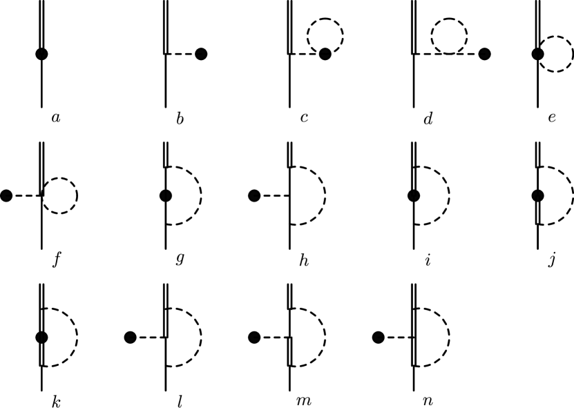
FIG. 1.: Relevant Feynman diagrams in the derivation of off-diagonal Goldberger-Treiman relation and its discrepancy. The filled circle denotes the pseudoscalar or pseudovector source. The double, solid and dashed lines correspond to the delta, nucleon and pion respectively.

REFERENCES

• [1] M. L. Goldberger and S. B. Treiman, Phys. Rev. 110, 1178 (1958).
• [2] R. Dashen and M. Weinstein, Phys. Rev. 118, 2330 (1969).
• [3] C. A. Dominguez, Phys. Rev. D 25, 1937 (1982); C. A. Dominguez, Riv. Nuovo Cim. 8, 1 (1985) and references therein.
• [4] V. Bernard, N. Kaiser and Ulf-G. Meissner, Phys. Rev. D 50, 6899 (1994).
• [5] T.R. Hemmert, B.R. Holstein, and N.C. Mukhopadyhay, Phys. Rev. D 51, 158 (1995).
• [6] V. Bernard et al., Nucl. Phys. A 635, 121 (1998).
• [7] J. L. Goity et al., Phys. Lett. B 454, 115 (1999).
• [8] E. Jenkins and A. V. Manohar, Phys. Lett. B 255, 558 (1991); B 259, 353 (1991).
• [9] Ulf-G. Meissner, Int. J. Mod. Phys. E 1, 561 (1992).
• [10] Jeffereson Laboratory experiment #E97-104, Measurement of the Parity Violating Asymmetry in the N to Delta Transition, S. P. Wells, N. Simicevic and K. Johnson, spokespersons (1997).
• [11] T. R. Hemmert, B. R. Holstein and J. Kambor, J. Phys. G 24, 1831 (1998).
• [12] D. R. T. Jones and S. T. Petcov, Phys. Lett. B 91, 137 (1980).
• [13] S. L. Adler, Ann. Phys. 50, 89 (1968); Phys. rev. D 12, 2644 (1975).
• [14] P. A. Schreiner and F. von Hippel, Nucl. Phys. B 38, 333 (1973) and references therein.
• [15] J. Gasser and H. Leutwyler, Nucl. Phys. B 250, 465 (1985).
• [16] N. Fettes and Ulf.-G. Meissner, Nucl. Phys. A 679, 629 (2001).
• [17] M. Dillig and M. Brack, J. Phys. G 5, 223 (1979).
• [18] S. J. Barish et al., Phys. Rev. D 19, 2521 (1979).
• [19] R. M. Davidson and N. C. Mukhopadhyay, Phys. Rev. D 42, 20 (1990); R. M. Davidson, N. C. Mukhopadhyay, and R. Wittman, ibid. 43, 71 (1991).
• [20] T. Ericson and W. Weise, Pions and Nuclei (Oxford Science, Oxford, England, 1988).
• [21] T. Kitagaki et al., Phys. Rev. D 42, 1331 (1990).
• [22] S. P. Wells, private communication.
• [23] Shi-Lin Zhu, C.M. Maekawa, G. Sacco, Barry R. Holstein, M.J. Ramsey-Musolf, Phys. Rev. D 65, 033001 (2001).
• [24] Shi-Lin Zhu, C.M. Maekawa, B.R. Holstein, and M.J. Ramsey-Musolf, Phys. Rev. Lett. 87, 201802 (2001).
• [25] R. Hasty et al, Science 290, 2117 (2000).
• [26] Shi-Lin Zhu, S.J. Puglia, B.R. Holstein, and M.J. Ramsey-Musolf, Phys. Rev. D 62, 033008 (2000).
• [27] R.D. McKeown and M.J. Ramsey-Musolf, hep-ph/0203011.
• [28] N.C. Mukhopadyhyay, et al., Nucl. Phys. A 633, 481 (1998).
Refer to caption