Non-Gaussianity in multi-field inflation

Abstract

This article investigates the generation of non-Gaussianity during inflation. In the context of multi-field inflation, we detail a mechanism that can create significant primordial non-Gaussianities in the adiabatic mode while preserving the scale invariance of the power spectrum. This mechanism is based on the generation of non-Gaussian isocurvature fluctuations which are then transfered to the adiabatic modes through a bend in the classical inflaton trajectory. Natural realizations involve quartic self-interaction terms for which a full computation can be performed. The expected statistical properties of the resulting metric fluctuations are shown to be the superposition of a Gaussian and a non-Gaussian contribution of the same variance. The relative weight of these two contributions is related to the total bending in field space. We explicit the non-Gaussian probability distribution function which appears to be described by a single new parameter. Only two new parameters therefore suffice in describing the non-Gaussianity.

I Introduction

The large scale structures of the universe are usually considered to arise from vacuum quantum fluctuations that are amplified during a stage of accelerated expansion. In its simplest version, inflation predicts the existence of an adiabatic initial fluctuation with Gaussian statistics and an almost scale-invariant spectrum [1]. And it is clear that as long as the evolution is linear from the radiation era, non-Gaussianity can arise only from an “initial” non-Gaussianity generated during inflation.

Simple calculations, that we reproduce in the second section of this paper, however show that within single field inflationary framework it is not possible to produce primordial non-Gaussian fluctuations if the slow-roll conditions are preserved throughout the inflationary period during which the seeds of the large-scale structures are generated. Non-Gaussianity can be generated only if the inflation starts from a non-vacuum initial state [18] or if there exist sharp features in the shape of the potential [19], but it in the latter case it clearly shows up in the density fluctuation power spectrum. It has been noticed however that the situation is somewhat changed when more than one light scalar field are present during inflation. In this case it is to be noticed first that one generically produces a mixture of adiabatic and isocurvature fluctuations [2, 3, 4, 5] that can be uncorrelated or correlated [6, 7, 8]. The observational consequences of the existence of these two types of modes have started to be considered [10, 11, 12] but they clearly depend on which type of matter each of the field decays to. Multi-field inflation also opens the door to the generation of non-Gaussianity simply because the non-linear couplings can be much stronger in the isocurvature direction than in the adiabatic direction [22, 23, 24, 21]. For instance in models in which a Peccei-Quinn symmetry is broken during inflation, it was pointed out by Allen et al. [13] that a fourth order derivative term in the effective theory leads to non-Gaussianity in the axion density. In the ”seed” models including $\chi^{2}$ [14], axion [13, 15], Goldstone bosons [16] and topological defects [17] models, there is a test scalar field that is a pure perturbation and that does not contribute to the background energy density; the energy being quadratic in the field, it induces non-Gaussianity in the perturbations. In such models however the non-Gaussian features are present in the isocurvature modes only and will be observationally relevant only if those modes survive the reheating phase. The phenomenological situation is somewhat different however if a transfer of the modes is possible, that is when the fields are coupled [25, 26].

The aim of this paper is therefore to explore whether in the context of multi field inflation it is possible to generate non-Gaussian features while preserving the adiabatic slow-roll type power spectrum and what would be its observational signature. We are obviously motivated by the development of Cosmic Microwave Background (CMB) and large scale structures observations that offer an opportunity reconstruct the properties of the primordial metric perturbations. Primordial fluctuations are more directly probed by CMB observations but then the number of modes that can be measured is still small. Up to now, no non-Gaussian signature has been detected in either the 4 year COBE data [27, 28] or the 1 year MAXIMA data [29]. In large-scale structure surveys the number of independent modes one can observe is large but the difficulty is that the non-linear gravitational dynamics [30] generates non-Gaussian couplings that can shadow the primordial ones [31]. One should then rely on a good understanding of the impact of the gravitational dynamics on the observations. Cosmic shear surveys might offer one of the most serious opportunity to explore such effects in the coming years [32, 33].

We start (Section II) by a general overview of the generation of non-Gaussianity in single and multi-field inflation. It will lead us to define a mechanism that can produce such non-Gaussianity. In Section III, we then consider the evolution of perturbations in two-field inflation and summarize how isocurvature perturbation can be transferred to the adiabatic component when the trajectory in the field space is curved. The isocurvature mode develops non-Gaussianity due to self-interaction; we study in Section IV the evolution of such a self-interacting field in an expanding universe. After having posed the problem for a quantum scalar field in an inflationary background we address this issue from a classical point of view. In Section V and  VI, we compute the probability distribution function that can be obtained in the class of models considered in this article.

II Overview of the mechanism

As explained in the introduction, our goal is to design a model that can produce sufficiently large non-Gaussianity at least for a band $[\lambda,\lambda+\Delta\lambda]$ of wavelengths observationally relevant, i.e. that corresponds to the large scale structure scales. To guide us in this task, we review the properties of non-Gaussianity in single field and multi-field inflation models in order to determine whether they fulfill our requirements.

Let us start by considering a single field, $\phi$, in slow-roll inflation. The Klein-Gordon equation for its perturbation is of the form

$$\ddot{\delta\phi}+3H\dot{\delta\phi}-\frac{\Delta}{a^{2}}\delta\phi=-V^{\prime\prime}\delta\phi-3V^{\prime\prime\prime}(\delta\phi)^{2}+\ldots$$ (1)

During the slow-roll regime, $|\dot{H}|\ll H^{2}$ and $\ddot{\phi}\ll 3H\dot{\phi}$ so that

$$3H^{2}M_{4}^{2}\simeq V,\qquad H\dot{\phi}\simeq-V^{\prime},$$ (2)

where $M_{4}$ is the reduced Planck mass, and the slow-roll conditions can be expressed as $\varepsilon\ll 1$ and $|\eta|\ll 1$ with

$$\varepsilon\equiv M_{4}\frac{V^{\prime}}{V},\qquad\eta\equiv M_{4}^{2}\frac{V^{\prime\prime}}{V}.$$ (3)

In order for the fluctuations of the scalar field to be large enough, one needs the mass of the field to be much smaller than $H$, in which case one gets $\delta\phi\sim H$. To get the correct amplitude for the primordial fluctuations, one needs $V^{3/2}/(V^{\prime}M_{4}^{3})\sim 10^{-5}$ so that

$$H\sim 10^{-5}\varepsilon M_{4}.$$ (4)

The band of wavelengths $[\lambda,\lambda+\Delta\lambda]$ corresponding to large scale structures exits the Hubble radius during the $e$-folds

$$N_{\lambda}=H\Delta t=\Delta\ln\lambda,$$ (5)

during which the slow-roll parameter $\eta$ has varied as $\Delta\eta\sim(\xi-\eta\varepsilon)\Delta\phi/M_{4}$, with $\xi\equiv M_{4}^{3}(V^{\prime\prime\prime}/V)$. From Eq. (4), one deduces that

$$\Delta\phi/M_{4}\sim-\varepsilon H\Delta t.$$ (6)

Now, if the quadratic term in the r.h.s. of Eq (1) is dominant over the linear term then $V^{\prime\prime}/V^{\prime\prime\prime}<\delta\phi\sim H$ and, using Eq (4), one deduces that $\Delta\eta>10^{5}\eta N_{\lambda}$. This will induce a rapid breakdown of the slow-roll inflation. This can be understood by the fact that the potential has to be both flat enough for the fluctuations to develop and steep enough for the non-linear terms not to be negligible. A way round to this argument is to consider potential with a sharp feature [19] but in that case the non-Gaussianity is associated with a departure from scale invariance and is located in a very small band of wavelengths.

Thus, one requires at least one auxiliary field. As a second situation let us consider the case in which this auxiliary field does not interact with the inflaton so that the potential has the form

$$V(\phi,\chi)=U(\phi)+\frac{1}{2}m^{2}\chi^{2}+\ldots$$ (7)

so that the cosmological evolution drives $\chi$ towards the minimum of its potential $\chi=0$. It follows that the lowest order contribution to its energy density perturbation is not given by the standard expression $\chi\delta\chi$ but one has to go to quadratic order. Thus, even if the Klein-Gordon equation is linear, the energy density of the field will develop non-Gaussianities with a $\chi^{2}$ statistics and with $\rho_{\chi}\sim H^{4}$. This energy has to be compared to the contribution of the inflaton $\rho_{\phi}\sim U\sim H^{2}M_{4}^{2}$. It follows that $\delta\rho_{\chi}/\delta\rho_{\phi}\sim 10^{-5}(m/H)^{2}$, so that the contributions of the auxiliary field to the background dynamics and to the Poisson equation are negligible. $\chi$ can develop non-Gaussianities but they are not transferred to the inflaton perturbation and gravitational potential.

The two fields have to interact, a prototypal example being a scattering term of the form $\mu\phi^{2}\chi^{2}$ as proposed in [24], so that there are a priori two sources of non-Gaussianities: (i) as in the previous case, the density of the field $\chi$ will be quadratic and (ii) due to the coupling, the Klein-Gordon equation for the field $\phi$ will get an source term in the r.h.s. of Eq. (1). Consider a potential of the form

$$V(\phi,\chi)=U(\phi)+\frac{1}{2}\mu\phi^{2}\chi^{2}+\frac{1}{2}m^{2}\chi^{2}+\frac{\lambda}{4!}\chi^{4},$$ (8)

so that the effective mass of the auxiliary field is $m^{2}_{\rm eff}=m^{2}+\mu\phi^{2}$. If initially $|\phi|>|\chi|$, $\chi$ will roll toward $\chi=0$ where it will stay so that $\phi$ drives the inflation and $H^{2}M_{4}^{2}\sim U$. For the auxiliary field to develop non negligible fluctuation, one needs that $m^{2}_{\rm eff}<H^{2}$. If $\mu>0$ then this implies that both $m^{2}$ and $\mu\phi^{2}$ have to be smaller than $H^{2}$; since during a period of $N_{\lambda}$ $e$-folds, using Eq. (6), the variation of the coupling contribution is of order $-2\mu\phi M_{4}\varepsilon N_{\lambda}$, so that it can be smaller than $H^{2}$ for a number of $e$-folds

$$N_{\lambda}<10^{-5}H/(\mu\phi),$$ (9)

during which $\delta\chi\sim H$. When $\mu<0$, the effective mass can be smaller than $H$ due to cancellation between $m$ and $\mu\phi^{2}$ but still, the variation of the mass has to be smaller than $H$ so that the condition (9) is a necessary condition whatever the sign of $\mu$.

The Klein-Gordon equation (1) now has two source terms ${\cal S}_{1}=\mu\chi\phi\delta\chi$ and ${\cal S}_{2}=\mu\chi^{2}\delta\phi$. The solution will take the form $\delta\phi=\delta\phi_{{}_{\rm H}}+\delta\phi_{{}_{\rm NG}}$ where $\delta\phi_{{}_{\rm H}}$ is the solution of the homogeneous equation and $\delta\phi_{{}_{\rm NG}}$ a particular solution. As will be detailed in Section IV.2, one expects that at Hubble scale crossing $\delta\phi_{{}_{\rm NG}}\sim N_{\lambda}{\cal S}/H^{2}$. It follows that for the first source term, $\delta\phi_{{}_{\rm NG}}\sim N_{\lambda}\mu\phi\chi^{2}/H^{2}\sim N_{\lambda}\mu\phi$. The amplitude of the homogeneous (Gaussian) solution is $\delta\phi_{{}_{\rm H}}\sim H$ so that $\delta\phi_{{}_{\rm NG}}\sim(\mu\phi/H)\delta\phi_{{}_{\rm H}}<10^{-5}\delta\phi_{{}_{\rm H}}$. The second source term gives rise to a solution $\delta\phi_{{}_{\rm NG}}\sim N_{\lambda}\mu\chi^{2}\delta\phi/H^{2}\sim N_{\lambda}\mu\delta\phi$; the coefficient $\mu$ cannot be of order unity since otherwise it will give a contribution of order $\mu\phi^{2}$ to the effective mass of $\chi$. Thus if $\mu$ is of order unity either $m_{\rm eff}<H$ so that $\chi\sim H$ but then it implies that $\phi/H<1$, which is not the case during inflation or $m_{\rm eff}>H$ but then $\chi\ll H$. It follows that in any situation the non-Gaussian correction is negligible compared to the Gaussian contribution.

Now, let us study the relative magnitude of the different terms entering the Poisson equation. First, $U_{,\phi}\delta\phi\sim\varepsilon H^{3}M_{4}$ while the interaction term is of order $V_{,\phi\chi}\chi\delta\phi\sim g^{2}\phi H^{3}<(10^{-10}/N_{\lambda})\varepsilon H^{3}M_{4}$ and is thus negligible. $V_{,\chi\chi}\chi^{2}$ has a contribution of order $\lambda\chi^{4}\sim(\lambda 10^{-5})\varepsilon H^{3}M_{4}$ which is negligible and a second contribution $g^{2}\phi^{2}\chi^{2}<(10^{-10}/N_{\lambda})(\phi/H)\varepsilon H^{3}M_{4}$ which is also negligible. Note also that the term $V_{,\chi}\chi\sim m^{2}_{\rm eff}\chi^{2}<H^{4}\sim 10^{-5}\varepsilon HM_{4}$, so that it is also subdominant.

It follows that even if $\chi$ develops non-Gaussianities and is coupled to the inflaton, the requirement that its effective mass is smaller than $H$ during a sufficient number of $e$-folds imply that it is negligible both in the Poisson equation and in the inflaton evolution equation.

As can be seen from the previous example, a quadratic interaction does not fulfill the requirements. We turn to a toy model in which the potential, in a neighborhood of the trajectory in field space, takes the form

$$V=U(\phi)+m^{2}_{\times}(\phi-\phi_{0})\chi+\frac{\lambda}{n!}\chi^{n}.$$ (10)

Indeed, this very unusual form with linear coupling tends to show that a particle physics realization of the scenario may be difficult to build and the potential (10) is just meant to be an effective potential. As in the previous example, we have to estimate the order of magnitude of the effect of $\chi$ both in the Poisson equation and in the equation of evolution of the inflaton. Imposing that the drift in the $\chi$ direction is smaller than in the $\phi$ direction during $N_{\lambda}$ $e$-folds gives that $N_{\lambda}<(H/m_{\times})^{2}$. The source term in the Klein-Gordon equation (1) of the inflaton is $m^{2}_{\times}\chi$ so that it gives rise to a contribution $\delta\phi_{{}_{\rm NG}}\sim N_{\lambda}m^{2}_{\times}/H<\delta\phi_{{}_{\rm H}}$ which can be of the same order as the homogeneous Gaussian solution $\delta\phi_{{}_{\rm H}}$. In the Poisson equation, the only new contribution is of order $V_{,\chi\phi}\delta\phi\chi\sim m^{2}_{\times}H^{2}<(10^{-5}/N_{\lambda})\varepsilon H^{3}M_{4}$ and is thus negligible compared to the contribution arising from $U$. As in the previous example, the self-interaction term will also turn out to be negligible. As a conclusion, such a potential will give rise to non-Gaussianities sourced by the coupling to the inflaton perturbation. In such a scenario, the field $\chi$ develops its non-Gaussianities due to non-linear evolution and these non-Gaussianities are transferred to the inflaton field due to the coupling source term in its Klein-Gordon equation. Note that it does not generate directly non-Gaussianities in the gravitational potential since its energy perturbation is always negligible.

In a neighborhood of the minimum of the potential given by $\chi_{0}(\phi)$, the potential can be developed in powers of $\chi-\chi_{0}(\phi)\equiv\delta\chi$ as $\alpha_{n}\delta\chi^{n}$. The first contribution is $\alpha_{2}\delta\chi^{2}$; either $\alpha_{2}>H^{2}$ and the fluctuation of $\chi$ will be negligible or $\alpha_{2}<H^{2}$ and one needs to consider next terms. If the cubic term is dominant then the trajectory $\chi_{0}(\phi)$ is unstable. Now if it is either negligible with the quartic order or of the same order, the latter situation resulting in the fine tuning $\alpha_{3}\sim\alpha_{4}H$. For the following $n>3$ terms, they will be associated with a particular solution of magnitude $\delta\phi_{{}_{\rm NG}}\sim\alpha_{n}\delta\chi^{n}/H^{2}\sim\alpha_{n}H^{n-4}\delta\phi_{{}_{\rm H}}$. The $n$th order term will have a non negligible contribution to $\delta\phi$ only if $\alpha_{n}\sim H^{4-n}$. Only for $n=4$ can $\alpha_{n}$ be a pure number that can be chosen of order unity. This is the only term for which the non-Gaussian fluctuations can develop on a long time scale without any tuning to $H$. This naturality arguments lead us to expect the most efficient and only relevant term to consider is an auxiliary field self-interacting with a quartic potential, $\lambda\chi^{4}/4!$, and coupled to the inflaton .

The sketch of the scenario will thus be the following. The auxiliary field develops non-Gaussianities. The bundle of field trajectories in the field space $(\phi,\chi)$ is deformed when the potential minimum is bent. According to the sign of $\lambda$, it is focalized ($\lambda>0$) or defocalized ($\lambda<0$) and the section of the bundle is deformed, as depicted on figure 1 (this completely analogous to the deformation of the section of bundle of light propagating in a gravitational field). Neighboring trajectories have different lengths so that the fluctuations along each of the trajectories will be slightly different.

To formalize this scenario, we describe in more details the coupling and transfer between adiabatic and isocurvature modes. To characterize the non-Gaussianity, one will need to treat the behavior of the quantum fluctuation before Hubble scale crossing. But, the trajectories after Hubble scale crossing can be treated classically and the classical contribution is expected to dominate over the quantum one if the bending occurs late enough after Hubble scale crossing. Note that the case in which $\lambda<0$ is less interesting since the trajectory becomes unstable; $\chi_{0}(\phi)$ corresponds to a maximum of the potential and we are more in situation like the one of a phase transition. We will however consider the case $\lambda<0$ while computing the PDF.

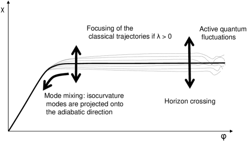
Figure 1: The trajectories of the fields in the plane ($\phi,\chi$), once smoothed on a scale $R$. Before Hubble scale crossing ($R<H$), the trajectories behave quantumly because the quantum fluctuations are active up to scale $H$ and are not smoothed out. After the Hubble scale crossing ($R>H$), the trajectories can be treated as classical trajectories. Note that this transition happens at different time for different values of $R$. The bundle of classical trajectories then evolves in the two dimensional potential and its cross section evolves with time. During the bending of the potential valley, the isocurvature modes project on the isocurvature modes and there is a transfer because the length of each trajectory is different depending on its position.

III Two-field inflation: adiabatic-isocurvature transfer

We describe, following mainly [7, 8], in this section the mixing between adiabatic and isocurvature modes in multi-field inflation which is one of the major element of our mechanism (see also e.g. [9] for an earlier study).

The class of multi-field inflationary models can be derived from a Lagrangian for $N$ scalar fields

$${\cal L}=-\frac{R}{16\pi G}+\frac{1}{2}\sum_{j=1}^{N}\partial_{\mu}\varphi_{j}\partial^{\mu}\varphi_{j}-V(\varphi_{1},\ldots,\varphi_{N})$$ (11)

where $G$ is the 4-dimensional Newtonian constant, $R$ the Ricci scalar and Greek indices run from 0 to 3. We describe the universe by a Friedmann-Lemaître spacetime with metric

$${\rm d}s^{2}=-{\rm d}t^{2}+a^{2}(t)\delta_{ij}{\rm d}x^{i}{\rm d}x^{j}$$ (12)

where $t$ is the cosmic time and $a$ the scale factor. We also introduce the conformal time $\eta$ defined by ${\rm d}t\equiv a{\rm d}\eta$. It follows that the Einstein equations take the form

$$H^{2}=\frac{4\pi G}{3}\left(\sum_{j=1}^{N}\dot{\varphi}_{j}^{2}+2V\right)$$ (13)

$$\dot{H}=-4\pi G\sum_{j=1}^{N}\dot{\varphi}_{j}^{2}$$ (14)

$$\ddot{\varphi}_{j}+3H\dot{\varphi}_{j}=-V_{j}$$ (15)

where a dot refers to a derivation with respect to the cosmic time, $t$, $H\equiv\dot{a}/a$ and $V_{j}$ refers to a derivation with respect to $\varphi_{j}$. We also set $M_{4}^{-2}\equiv 8\pi G$.

Let us consider the simplest case in which we have only two scalar fields $\varphi_{1}$ and $\varphi_{2}$. We decompose these two fields on the direction tangent ($\sigma$)and perpendicular ($s$) to the trajectory as

$$\pmatrix{\dot{\sigma}\cr\dot{s}}={\cal M}(\theta)\pmatrix{\dot{\varphi}_{1}\cr\dot{\varphi}_{2}},\qquad{\cal M}(\theta)\equiv\pmatrix{\cos\theta&\sin\theta\cr-\sin\theta&\cos\theta}$$ (16)

the angle $\theta$ being defined by

$$\cos\theta\equiv\frac{\dot{\varphi}_{1}}{\sqrt{\dot{\varphi}_{1}^{2}+\dot{\varphi}_{2}^{2}}},\qquad\sin\theta\equiv\frac{\dot{\varphi}_{2}}{\sqrt{\dot{\varphi}_{1}^{2}+\dot{\varphi}_{2}^{2}}}$$ (17)

from which it can be deduced that $s$ is constant along the trajectory. The evolution of the field is obtained by combining the two Klein-Gordon equations (15)

$$\pmatrix{\ddot{\sigma}\cr\ddot{s}}+3H\pmatrix{\dot{\sigma}\cr\dot{s}}+{\cal M}(\theta)\pmatrix{V_{1}\cr V_{2}}=0$$ (18)

and the Friedmann equation is

$$H^{2}=\frac{4\pi G}{3}\left[\dot{\sigma}^{2}+2V(\sigma,s={\rm constant})\right].$$ (19)

The interpretation of the fields $\sigma$ and $s$ as the adiabatic and isocurvature components of $(\varphi_{1},\varphi_{2})$ will arise from the following study of the perturbations evolution and properties. At linear order, the perturbed metric takes the form [1]

$${\rm d}s^{2}=-(1+2A){\rm d}t^{2}+2a(t)\partial_{i}B{\rm d}x^{i}{\rm d}t+a^{2}(t)[(1-2C)\delta_{ij}+2\partial_{ij}E]{\rm d}x^{i}{\rm d}x^{j}$$ (20)

where $A$, $B$, $C$ and $E$ are four scalar perturbations and we expand the scalar fields as

$$\varphi_{i}(t,x^{j})=\varphi_{i}+\delta\varphi_{i}(t,x^{j}).$$ (21)

We can introduce two sets of gauge invariant variables. The Newtonian or longitudinal gauge is defined as

$$B=E=0,\qquad A=\Phi,\qquad C=\Psi,\qquad\delta\varphi_{i}=\chi_{i}.$$ (22)

We introduce the perturbation of the inflaton in the flat slicing gauge ($C=0,E=0$) by

$$Q_{i}=\chi_{i}+\frac{\dot{\varphi}_{i}}{H}\Phi.$$ (23)

In Newtonian gauge, the evolution equations in Fourier space reduce to the set

$$\Phi=\Psi$$ (24)

$$\dot{\Phi}+H\Phi=\frac{1}{2M_{4}}(\dot{\varphi}_{1}\chi_{1}+\dot{\varphi}_{2}\chi_{2})$$ (25)

$$-\frac{\Delta}{a^{2}}\Phi+3H\dot{\Phi}+(3H^{2}+\dot{H})\Phi=-\frac{1}{2M_{4}}(V_{1}\chi_{1}+\dot{\varphi}_{1}\chi_{1}+V_{2}\chi_{2}+\dot{\varphi}_{2}\chi_{2})$$ (26)

$$\ddot{\chi}_{i}+3H\dot{\chi}_{i}-\frac{\Delta}{a^{2}}\chi_{i}+V_{ij}\chi_{j}=-2V_{i}\Phi+4\dot{\varphi}_{i}\Phi.$$ (27)

By construction, ${\delta\!s}$ is gauge invariant so that $Q_{s}=\chi_{s}={\delta\!s}$ and from Eq. (23), $Q_{\sigma}=\chi_{\sigma}+\dot{\sigma}\Phi/H$. Using that

$$^{t}\dot{\cal M}=-\dot{\theta}{}^{t}\dot{\cal M}J,\qquad^{t}\ddot{\cal M}=-\ddot{\theta}{}^{t}\dot{\cal M}J-\dot{\theta}^{2}{}^{t}\dot{\cal M},\qquad J\equiv\pmatrix{0&1\cr-1&0},$$ (28)

the Klein-Gordon equations (27) can be rewritten as

$$\pmatrix{\chi_{\sigma}\cr{\delta\!s}}^{..}+3H\pmatrix{\chi_{\sigma}\cr{\delta\!s}}^{.}+\left[-\frac{\Delta}{a^{2}}-\dot{\theta}^{2}+{\cal M}V_{ij}{}^{t}{\cal M}\right]\pmatrix{\chi_{\sigma}\cr{\delta\!s}}=2\dot{\theta}J\pmatrix{\chi_{\sigma}\cr{\delta\!s}}^{.}$$

$$\qquad\qquad\qquad\qquad\qquad+(\ddot{\theta}+3H\dot{\theta})J\pmatrix{\chi_{\sigma}\cr{\delta\!s}}-2\Phi{\cal M}\pmatrix{V_{1}\cr V_{2}}+4\Phi\pmatrix{\dot{\sigma}\cr 0}$$ (29)

and the Poisson equation (26) takes the form

$$-\frac{\Delta}{4\pi Ga^{2}}\Phi=2\dot{\theta}\dot{\sigma}{\delta\!s}+\ddot{\sigma}\chi_{\sigma}-\dot{\sigma}(\dot{\chi}_{\sigma}-\dot{\sigma}\Phi).$$ (30)

Defining the mass matrix $U$ of the two fields $(\sigma,s)$ as

$$\pmatrix{U_{\sigma\sigma}&U_{\sigma s}\cr U_{s\sigma}&U_{ss}}\equiv{\cal M}V_{ij}{}^{t}{\cal M},\qquad\hbox{and}\qquad\pmatrix{U_{\sigma}\cr U_{s}}={\cal M}\pmatrix{V_{1}\cr V_{2}}$$ (31)

and making use of (30), the system (III) takes the form

$$\ddot{\chi}_{\sigma}+3H\dot{\chi}_{\sigma}+\left(-\frac{\Delta}{a^{2}}-\dot{\theta}^{2}+U_{\sigma\sigma}\right)\chi_{\sigma}=-2\Phi U_{\sigma}+4\dot{\sigma}\Phi+2(\dot{\theta}{\delta\!s})^{.}-2\frac{\dot{\theta}}{\dot{\sigma}}U_{\sigma}{\delta\!s}$$ (32)

$$\ddot{{\delta\!s}}+3H\dot{\delta s}+\left(-\frac{\Delta}{a^{2}}-\dot{\theta}^{2}+U_{ss}\right){\delta\!s}=-\frac{\dot{\theta}}{\dot{\sigma}}\frac{\Delta}{2\pi Ga^{2}}\Phi.$$ (33)

The comoving curvature perturbation is given by

$${\cal R}\equiv C+\frac{H}{\rho+P}(\dot{\varphi}_{1}\delta\varphi_{1}+\dot{\varphi}_{2}\delta\varphi_{2})=C+\frac{H}{\dot{\sigma}}\delta\sigma=\frac{H}{\dot{\sigma}}Q_{\sigma}$$ (34)

from which it is deduced that

$$\dot{\cal R}=-\frac{H}{\dot{H}}\frac{\Delta}{a^{2}}\Phi+2\frac{H}{\dot{\sigma}}\dot{\theta}{\delta\!s}.$$ (35)

It follows from this analysis that as long as $\dot{\theta}=0$, ${\delta\!s}$ evolves as a test scalar field evolving in an unperturbed Friedmann-Lemaître universe and does not affect the evolution of the gravitational perturbations; $\Phi$ couples solely to the fluctuation of $\sigma$ in Eq. (30). It is recovered that the entropy remains constant on super-Hubble scales as long as there is no mixing. ${\delta\!s}$ will transfer energy to the gravitational potential only when $\dot{\theta}\not=0$ and the comoving curvature can be affected significantly even on super-Hubble scales if the fields follow a curved trajectory. Note that this mechanism is effective only during the inflationary period.

The “surviving” isocurvature perturbations (all of them in the case where there is no bending) needs to be taken into account. At the end of the inflationary period, both the inflaton and auxiliary field will decay into particles and radiation. To set the initial conditions in the radiation era, one needs to specify in details these decays. When there is no bending of the trajectory, this is the only mechanism through which an imprint of the isocurvature modes can survive. According to the scenario, the initial perturbations in the cosmic fluids at the beginning of the radiation era are a mixture of adiabatic and isocurvature modes that can be correlated (see e.g. [6, 7]). In full generality, we will have to consider both contributions but we focus in the following on the “pure” case where the fluctuations at the end of inflation are strictly adiabatic, which can occur if the two fields decay identically.

IV Generation of non-Gaussianity

The goal of this section is to estimate the magnitude of the non-Gaussianity developed by the isocurvature mode during a phase of de Sitter inflation. The frame in which such calculations should be performed is the quantum field theory for a coupled scalar field. As we are interested in the emergence of weak non-Gaussian features, through for instance the emergence of non-zero connected part of high order correlation function, a perturbation theory approach should be applicable in principle.

We point out however that a series of technical or conceptual problems emerge in this physical situation for which there seems to exist no known solution. We first present in which way the computation we would like to do is affected by those problems but, as their resolution goes far beyond the estimate we would like to obtain, we finally turn to a classical treatment of the field behavior. This provides a solid enough ground to estimate the amounts of non-Gaussianities at scales that remain super-Hubble a time long enough before the adiabatic-isocurvature mode transfer.

IV.1 The quantum level calculation

As seen from the previous investigation, the entropy field ${\delta\!s}$ is decoupled from the gravitational perturbations and can be considered as a test field evolving in an homogeneous and isotropic cosmological universe. To characterize the statistical properties of such a self-interacting field, one would ideally like to compute its high-order correlation functions. The inflationary phase can be described by a de Sitter spacetime [34] in flat spatial section slicing

$${\rm d}s^{2}=\frac{1}{(H\eta)^{2}}\left(-{\rm d}\eta^{2}+\delta_{ij}{\rm d}x^{i}{\rm d}x^{j}\right)$$ (36)

which is conformal to half of the Minkowski spacetime. The conformal time is related to the cosmological time by

$$\eta=-\frac{1}{H}\hbox{e}^{-Ht}$$ (37)

and runs from $-\infty$ to 0, the limit $\eta\rightarrow 0^{-}$ representing the “infinite future”. The de Sitter spacetime can be viewed as a four dimensional hyperboloid embedded in a five dimensional Minkowski spacetime

$$-\left(x_{0}\right)^{2}+\left(x_{1}\right)^{2}+\left(x_{2}\right)^{2}+\left(x_{3}\right)^{2}+\left(x_{4}\right)^{2}=1/H^{2}.$$ (38)

The invariance of this surface under five dimensional Lorentz transformations implies that the de Sitter space enjoys a 10 parameter group of isometries known as the de Sitter group $O(4,1)$. It is usual to define the de Sitter length function $z(x,y)$ by $H^{2}(x-y)^{2}/2=1-z(x,y)$ where $x$ and $y$ are the five dimensional coordinates of two points on the hyperboloid (38). It follows that $z(x,y)=H^{2}xy$ and the two points are timelike or spacelike separated respectively when $z>1$ and $z<1$

For a minimally coupled free quantum field of mass $m$, due to the spatial translation invariance, the solution can be decomposed in plane waves as

$$\widehat{v}_{0}({\bf x},\eta)=\int\frac{{\rm d}^{3}{\bf k}}{(2\pi)^{3/2}}\left[v_{0}(k,\eta)\widehat{b}_{\bf k}\hbox{e}^{i{\bf k}\cdot{\bf x}}+v^{*}_{0}(k,\eta)\widehat{b}_{\bf k}^{\dagger}\hbox{e}^{-i{\bf k}\cdot{\bf x}}\right]$$ (39)

where we have introduced $\widehat{v}\equiv a\,\widehat{\delta\!s}$, a hat referring to an operator. In this Heisenberg picture, the field has become a time-dependent operator expanded in terms of time-independent creation and annihilation operators satisfying the usual commutation relations $[\widehat{b}_{\bf k},\widehat{b}_{{\bf k}^{\prime}}^{\dagger}]=(2\pi)^{3}\delta^{(3)}({\bf k}-{\bf k}^{\prime})$. We can then define the free vacuum state by the requirement

$$\widehat{b}_{\bf k}\left|0\right>=0\qquad\hbox{for all}\qquad{\bf k}.$$ (40)

As it is standard while working in curved space [35], the definition of the vacuum state suffers from some arbitrariness since it depends on the choice of the set of modes $v_{0}(k,\eta)$. They satisfy the evolution equation

$$v_{0}^{\prime\prime}+\left(k^{2}-\frac{2}{\eta^{2}}-\frac{m^{2}/H^{2}}{\eta^{2}}\right)v_{0}=0,$$ (41)

the general solution of which is given by $\sqrt{\pi\eta/4}\left[c_{1}H^{(1)}_{\nu}(k\eta)+c_{2}H^{(2)}_{\nu}(k\eta)\right]$ with $|c_{2}|^{2}-|c_{1}|^{2}=1$, where $H^{(1)}_{\nu}$ and $H^{(2)}_{\nu}$ are the Hankel functions of first and second kind and with $\nu^{2}=9/4-m^{2}/H^{2}$. Among this family of solutions, it is natural to choose the one enjoying the de Sitter symmetry and the same short distance behavior than in flat spacetime. This leads to

$$v_{0}(k,\eta)=\frac{1}{2}\sqrt{\pi\eta}H^{(2)}_{\nu}(k\eta).$$ (42)

This uniquely defines a de Sitter invariant vacuum state referred to as the Bunch-Davies state vacuum [35]. In the massless limit, the solution (41) reduces to

$$v_{0}(k,\eta)=\left(1-\frac{{\rm i}}{k\eta}\right)\frac{\hbox{e}^{-{\rm i}k\eta}}{\sqrt{2k}}.$$ (43)

Having determined the free field solutions, one can then aim to express the $N$-point correlation functions of the interacting field, ${\delta\!s}_{i}$, in terms of those of the free scalar field. For instance, on the example of a ${\delta\!s}^{4}$ theory, the connected part of the 4-point correlator of the interacting field will reduce, at lowest order, to

$$\left<0\right|T\widehat{\delta\!s}_{i}({\bf x}_{1},\eta_{1})\ldots\widehat{\delta\!s}_{i}({\bf x}_{4},\eta_{4})\left|0\right>={\rm i}\frac{\lambda}{4!}\int\left<0\right|T\widehat{\delta\!s}({\bf x}_{1},\eta_{1})\widehat{\delta\!s}({\bf x}_{2},\eta_{2})\widehat{\delta\!s}({\bf x}_{3},\eta_{3})\widehat{\delta\!s}({\bf x}_{4},\eta_{4})\widehat{\delta\!s}^{4}({\bf x},\eta)\left|0\right>\sqrt{-g}\,{\rm d}^{4}{\bf x}\,{\rm d}\eta.$$ (44)

Using the Wick theorem and keeping only the connected part leads to

$$\left<0\right|T\widehat{\delta\!s}_{i}({\bf x}_{1},\eta_{1})\ldots\widehat{\delta\!s}_{i}({\bf x}_{4},\eta_{4})\left|0\right>={\rm i}\frac{\lambda}{4!}\int\prod_{i=1}^{4}G({\bf x},\eta;{\bf x}_{i},\eta_{i})\sqrt{-g}{\rm d}^{3}{\bf x}{\rm d}\eta.$$ (45)

$G({\bf x},\eta;{\bf x}^{\prime},\eta^{\prime})$ is the free propagator, that is the time ordered product of two free fields in the free vacuum

$${\rm i}\,G({\bf x},\eta;{\bf x}^{\prime},\eta^{\prime})=\frac{1}{a(\eta)a(\eta^{\prime})}\int\frac{{\rm d}^{3}{\bf k}}{(2\pi)^{3}}\left[v_{0}(k,\eta)v_{0}^{*}(k,\eta^{\prime})\hbox{e}^{-{\rm i}{\bf k}.\Delta{\bf x}}\theta(-\Delta\eta)+v_{0}(k,\eta^{\prime})v_{0}^{*}(k,\eta)\hbox{e}^{{\rm i}{\bf k}.\Delta{\bf x}}\theta(\Delta\eta)\right]$$ (46)

with $\Delta{\bf x}\equiv{\bf x}^{\prime}-{\bf x}$ and $\Delta\eta\equiv\eta^{\prime}-\eta$ and $\theta$ being the Heavyside function. After integration over angles the free propagator can be computed [37] to be

$${\rm i}\,G({\bf x},\eta;{\bf x}^{\prime},\eta^{\prime})=\frac{H^{2}}{4\pi^{2}}\left(\frac{\eta\eta^{\prime}}{\Delta{\bf x}^{2}-\Delta\eta^{2}}+1+\int_{0}^{\infty}\frac{{\rm d}k}{k}\cos(k\Delta x)\hbox{e}^{-{\rm i}k|\Delta\eta|}\right).$$ (47)

While trying to compute the 4-point correlator (46) with the latter expression of the free field propagator (47), one has to face the existence of two infrared (IR) divergences. Note that at coinciding points, there is a UV divergence that can be regularized by taking into account that inflation started at a given initial time [36].

The IR logarithmic divergence at $k=0$ was first exhibited by Ford and Parker [38]. Allen and Folacci [39] showed that this divergence arises from the incorrect assumption of de Sitter invariance for the vacuum and from the existence of a zero mode, i.e. the action is invariant under transformations of the form $\phi\rightarrow\phi+{\rm constant}$. It is well known that an expansion in terms of creation and annihilation operators as in Eq. (39) is inadequate for the zero modes [40] in the same way as the expansion in terms of creation and annihilation operators for the standard quantum harmonic oscillator breaks down when the frequency is going to zero. To be slightly more precise, let us recall [41] the properties of a free massless scalar field leaving on a 3-torus of volume $V$. Beside the standard plane wave solutions associated to the creation and annihilation operators, $\widehat{b}_{\bf k}$ and $\widehat{b}_{\bf k}^{\dagger}$ obtained for ${\bf k}\not=0$ and describing harmonic oscillator of frequency $|{\bf k}|$, a complete set of solutions requires to consider the solution $(\widehat{x}_{0}+\widehat{p}_{0}t)/\sqrt{V}$ obtained for ${\bf k}=0$ and describing the classical solution for a free particle. The position and momentum operators $\widehat{x}_{0}$ and $\widehat{p}_{0}$ satisfy the commutation relation $[\widehat{x}_{0},\widehat{p}_{0}]={\rm i}$. A vacuum state can then be defined by imposing $\widehat{p}_{0}\left|0\right>=0$ and $\widehat{b}_{\bf k}\left|0\right>=0$. This state is the product of Fock and a Hilbert space corresponding respectively to the oscillators and the free particle (see e.g. [40, 41, 42, 43, 44]) and will not be normalizable. For a flat space in more than two dimensions, the continuum limit exists because the contribution of the zero mode is of zero measure, the volume of the phase space cancelling the divergence but the effect remains in de Sitter space whatever its dimension.

This divergence led some authors [39, 43, 45] to define other vacua with less symmetry than the de Sitter group but with a well defined propagator. For instance, in the closed spatial section slicing a natural choice is the $O(4)$ invariant vacuum [39] that is symmetric under rotations of the constant time hypersurfaces. The modes are discrete and the IR divergence is avoided by choosing a set of modes with a different solution for ${\bf k}=0$. Kirsten and Garriga [43] proposed the construction of an acceptable de Sitter invariant vacuum in which the zero mode is well treated. The case of de Sitter space with static spatial sections slicing was considered by Polarski [45]. In the case of flat spatial sections slicing, which we are most interested in, the IR problem can be regularized by working on a torus [37] with $-H^{-1}/2<x^{i}\leq H^{-1}/2$ which is equivalent to set an infrared cut-off. With such a regularization, this yields the result

$${\rm i}G({\bf x},\eta;{\bf x}^{\prime},\eta^{\prime})=\frac{H^{2}}{4\pi^{2}}\left(\frac{\eta\eta^{\prime}}{\Delta{\bf x}^{2}-\Delta\eta^{2}}-\frac{1}{2}\ln H^{2}(\Delta{\bf x}^{2}-\Delta\eta^{2})+{\rm constant}\right).$$ (48)

A second IR divergence arises at late time, i.e. when $\eta\rightarrow 0^{-}$ since the integral (46) with the regularized propagator (48) diverges due to the volume factor $1/H^{4}\eta^{4}$. The former resolution of the IR divergence in ${\bf k}=0$ cannot resolve this late time IR divergence. Tsamis and Woodard [37] pointed out that such correlation functions suffers from a series of flaws: (1) they are not finite even at lowest order, this problem becoming worth as the number of vertices grows, (2) it is not purely imaginary so that it implies a tree-order breakdown of unitarity. The physical origin seems to be the redshifting that drives all physical momenta toward zero when $\eta\rightarrow 0$, making the overlap between plane waves very strong. It is to be noted that the use of the regularized propagator given in Eq. (48) does not cure the problem nor the introduction of a late time cut-off (the existence of which could be associated with the reheating time).

The resolution of these fundamental problems goes far beyond the estimates we want to obtain on the effects of nonlinear couplings. We thus adopt a simpler approach assuming that at scales that exceed the Hubble size the field value trajectories are classical (e.g. deterministic) and encoded in the potential shape. Because the trajectories might have a non-trivial dependence with the initial field values set up at Hubble scale crossing, non-Gaussianities can be induced during that period. If the time between Hubble crossing and the bending of the trajectory is long enough the non-Gaussianities of such classical origin are going to exceeds those a priori present in the initial value distribution as tit emerges from the quantum process.

IV.2 The classical limit

To implement this idea, we consider the field ${\delta\!s}$ at a large enough scale. It amounts to applying to the evolution equation of the field a filtering procedure at a fixed (comoving) scale, $R$. In the following we note ${\underline{\delta}\!s}$ the filtered field (what exactly is the function it has been convolved with is not important). At the time the Hubble size has shrunk below the smoothing length, the trajectory of the field becomes classical. Its evolution equation is simply,

$$\ddot{{\underline{\delta}\!s}}+3H\dot{{\underline{\delta}\!s}}=\underline{\cal S}({\delta\!s}).$$ (49)

It derives from the real space Klein-Gordon equation applied for ${\delta\!s}$ [e.g. Eq. (33)] where the Laplacian term has been dropped on super-Hubble scales. Assuming that the trajectory of the mean field value in a super-Hubble patch is insensitive to the small scale fluctuations  we can replace $\underline{\cal S}({\delta\!s})$ by ${\cal S}({\underline{\delta}\!s})~{}$. In the absence of source terms in Eq. (49), ${\underline{\delta}\!s}$ is simply constant (e.g. trajectories are parallel lines on Fig. 1) and its value is given by its initial value set up at Hubble crossing. The initial value is given by a sum of Gaussian distributed values and non-Gaussian corrections induced by the non-linear couplings during the sub-Hubble evolution of the field,

$${\underline{\delta}\!s}_{\rm init.}={\underline{\delta}\!s}^{(0)}+{\underline{\delta}\!s}^{({\rm ng})}.$$ (50)

The resolution of Eq. (49) requires in general the knowledge of the source term. It can be solved however perturbatively if one assumes that ${\underline{\delta}\!s}$ can be expanded in terms of the coupling constant entering the source term,

$${\underline{\delta}\!s}(t)={\underline{\delta}\!s}^{(0)}+{\underline{\delta}\!s}^{(1)}+\dots$$ (51)

The evolution equation for ${\underline{\delta}\!s}^{(1)}$ is trivial to obtain. It reads,

$$\ddot{{\underline{\delta}\!s}}^{(1)}+3H\dot{{\underline{\delta}\!s}}^{(1)}={\cal S}({\underline{\delta}\!s}^{(0)})$$ (52)

the solution of which is

$${\underline{\delta}\!s}^{(1)}(t)={\underline{\delta}\!s}^{({\rm ng})}+(t-t_{\rm H})\frac{{\cal S}({\underline{\delta}\!s}^{(0)})}{3\,H},$$ (53)

which can be rewritten as

$${\underline{\delta}\!s}^{(1)}(t)={\underline{\delta}\!s}^{({\rm ng})}+N_{R}\,\frac{{\cal S}({\underline{\delta}\!s}^{(0)})}{3\,H^{2}},$$ (54)

where $N_{R}$ is the number of $e$-folds from the Hubble size crossing, $t_{H}$, to the time $t$. If the latter is large enough one expects the second term of this equation to dominate the first, e.g. that non-Gaussian effects induced during the classical evolution dominates those built during the stage of the quantum evolution. We will make this hypothesis in the following.

It clearly implies, as we anticipated in part II, that the amplitude of the first order corrective term is given by the amplitude of the source term ${\cal S}({\underline{\delta}\!s}^{(0)})$ divided by $H^{2}$ times the number of $e$-fold during which the non linear couplings are active.

The existence of such corrective terms are obviously of importance for the statistical properties of the field. If the source term contains nonlinear couplings the field ${\underline{\delta}\!s}$ is no more Gaussian. Such properties should be exhibited in the high order correlation function of the field. Exploring these consequences is the aim of the next section.

V Isocurvature modes Probability distribution function

As seen from the previous analysis, nothing prevents the isocurvature modes to develop non-Gaussian properties on super-Hubble scales. As stressed before, if the time between Hubble radius crossing and the exchange of modes is large enough, the properties of those modes will be determined by their stochastic evolution at super-Hubble scale, not so much by the quantum state with which the field modes reach super-Hubble scales. In other words we expect the high order correlation functions present in the quantum field to be finally superseeded by the ones induced by the subsequent stochastic couplings.

The aim of this section is then to characterize the way the non-Gaussian features in the isocurvature modes are built up. There are obviously many ways of characterizing non-Gaussian features in a stochastic field. The simplest approach is to consider the shape of the one-point probability distribution of the local field value. This series depends obviously in the type of couplings one has. For the reasons previously detailed, we will consider only the case of quartic couplings.

In the first part of this section (§ V.1) we show how it is possible to compute any of such cumulants at leading order in the coupling constant (that would correspond to tree-order calculation in a quantum field formulation). It finally leads to the expression of the generating function of the one-point cumulants (§ V.2).

To get insights into the physical interpretation of the previous results we then present (§ V.3) the derivation of a quantity more directly related to observations: the one-point PDF of the local field value. Not surprisingly we will see that the rare event tails of those distribution differs from those expected for a Gaussian distribution. Depending on the sign of the quartic coupling, one expects an excess or a deficit of rare values.

V.1 The expression of the fourth order cumulant

Let us focus on the case of a stochastic field ${\delta\!s}$ self-interacting with a potential,

$$V({\delta\!s})={\lambda\over 4!}\,{\delta\!s}^{4}$$ (55)

and we assume that the coupling constant $\lambda$ is small compared to unity. In the ${\underline{\delta}\!s}$ expansion, Eq. (51), it means that ${\delta\!s}^{(n)}$ is of the order of $\lambda^{n}$. We then consider the evolution equation (49) with

$${\cal S}({\underline{\delta}\!s})=-\frac{\lambda}{3!}{\underline{\delta}\!s}^{3}.$$ (56)

At this stage it should be noted that when using the ${\underline{\delta}\!s}$ field in the source term, one neglects the effects of the small scale fluctuations in the field trajectory. This is of no consequence for tree order calculations, however, no loop terms, that involve arbitrarily small scales fluctuations, can be reliably computed from this approach. If one wants to do that one should solve the full quantum problem. In this study we allow ourselves to use this simplification but forbid ourselves to compute correlation properties beyond tree order.

As said before in the absence of coupling the free field solution ${\underline{\delta}\!s}^{(0)}$ is time independent. This is not the case of higher order terms. For instance from Eq. (54), we know that for this coupling term,

$${\underline{\delta}\!s}^{(1)}=-{\lambda\over 18}\,N_{R}{\left[{\underline{\delta}\!s}^{(0)}\right]^{3}\over H^{2}},$$ (57)

a term which induces non-Gaussian properties in the field. In case of a quartic coupling the value of ${\underline{\delta}\!s}$ remains symmetric distributed so that the third order cumulant is always zero. The first non-vanishing high order cumulant is then the fourth one. Its value can be computed at leading order (in the coupling constant) from the expression of ${\underline{\delta}\!s}^{(1)}$. Indeed the fourth order cumulant is formally given by,

$$\left\langle{\underline{\delta}\!s}^{4}\rangle_{c}\equiv\langle{\underline{\delta}\!s}^{4}\right\rangle-3\left\langle{\underline{\delta}\!s}^{2}\right\rangle^{2}=\left\langle\left[{\underline{\delta}\!s}^{(0)}+{\underline{\delta}\!s}^{(1)}+\dots\right]^{4}\right\rangle-3\left\langle\left[{\underline{\delta}\!s}^{(0)}+{\underline{\delta}\!s}^{(1)}+\dots\right]^{2}\right\rangle^{2},$$ (58)

replacing ${\underline{\delta}\!s}$ by its expansion in the coupling constant, Eq. (51). The computation of these moments up to linear order in $\lambda$ gives,

$$\left\langle{\underline{\delta}\!s}^{4}\right\rangle_{c}=\left\langle\left[{\underline{\delta}\!s}^{(0)}\right]^{4}\right\rangle-3\left\langle\left[{\underline{\delta}\!s}^{(0)}\right]^{2}\right\rangle^{2}+4\left[\left\langle{\underline{\delta}\!s}^{(1)}\left[{\underline{\delta}\!s}^{(0)}\right]^{3}\right\rangle-3\left\langle{\underline{\delta}\!s}^{(1)}{\underline{\delta}\!s}^{(0)}\right\rangle\left\langle\left[{\underline{\delta}\!s}^{(0)}\right]^{2}\right\rangle\right].$$ (59)

This first two terms of this expression cancel because ${\underline{\delta}\!s}^{(0)}$ obeys a Gaussian statistics. One can finally check that the latter expression gives the connected part of $\left\langle{\underline{\delta}\!s}^{(1)}\left[{\underline{\delta}\!s}^{(0)}\right]^{3}\right\rangle$ so that, at leading order, the fourth order cumulant is given by,

$$\left\langle{\underline{\delta}\!s}^{4}\right\rangle_{c}=4\left\langle{\underline{\delta}\!s}^{(1)}\left[{\underline{\delta}\!s}^{(0)}\right]^{3}\right\rangle_{c}$$ (60)

which can be easily computed from the expression of ${\underline{\delta}\!s}^{(1)}$, so that,

$$\left\langle{\underline{\delta}\!s}^{4}\right\rangle_{c}=-{4\lambda\over 3}\,{N_{R}\over H^{2}}\left\langle\left[{\underline{\delta}\!s}^{(0)}\right]^{2}\right\rangle^{3}.$$ (61)

It is clear that at leading order the expression of the fourth order cumulant involves only the expression of ${\underline{\delta}\!s}^{(1)}$. All higher order terms in the expression of ${\underline{\delta}\!s}$ contribute only at higher order in $\lambda$ to this cumulant, and they would correspond to loop term corrections, e.g. Fig. 2.

However if one wishes to compute the expression of higher order cumulants, such as the sixth order one, the higher order terms in the expansion of ${\underline{\delta}\!s}$ will then contribute (still at tree order!), see Fig. 3. In the next subsection we explore in more details the mathematical structure of the cumulant hierarchy.

V.2 The structure of the field cumulants

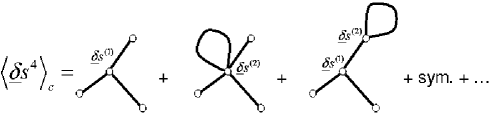
Figure 2: Diagrammatic representation of the fourth order cumulant in a perturbation theory approach. Lines correspond to connected pair points in ensemble averages of product of Gaussian variables as an application of the Wick theorem. End points are taken at zero order in the coupling constant (they are linear in the initial Gaussian field). Points at first order in the coupling constant are cubic in the field, at second order they are quintic, etc. The first diagram corresponds to the tree order term. It involves only one vertex. The other two diagrams correspond to loop corrections.

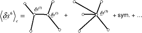
Figure 3: Diagrammatic representation of the sixth order cumulant at leading order. Two types of diagrams appear, one with two three-leg vertices, one with one five-leg vertex.

To get insights in how the leading order expression can be computed, it is useful to consider one where terms of various order in the expansion of ${\underline{\delta}\!s}$ are mixed together.

For instance the sixth order cumulant is, at leading order in $\lambda$, given by

$$\left\langle{\underline{\delta}\!s}^{6}\right\rangle_{c}=30\,\left\langle\left[{\underline{\delta}\!s}^{(1)}\right]^{2}\left[{\underline{\delta}\!s}^{(0)}\right]^{4}\right\rangle_{c}+6\,\left\langle{\underline{\delta}\!s}^{(2)}\left[{\underline{\delta}\!s}^{(0)}\right]^{5}\right\rangle_{c}$$ (62)

since ${\underline{\delta}\!s}^{(2)}$ scales like $\lambda^{2}\left[{\underline{\delta}\!s}^{(0)}\right]^{5}$. The factors that appear in these expressions correspond to the number of each of such terms that appear in those expansions.

In general the tree order term of any cumulant is determined by the consequences of the Wick theorem applied to ${\underline{\delta}\!s}^{(0)}$. It will therefore be of the form,

$$\left\langle{\underline{\delta}\!s}^{n}\right\rangle_{c}=\sum_{\rm decompositions}\left\langle\prod_{i=1}^{n}{\underline{\delta}\!s}^{(p_{i})}\dots{\underline{\delta}\!s}^{(p_{n})}\right\rangle_{c}$$ (63)

where all the decompositions are such that

$$\sum_{i=1}^{n}(2p_{i}+1)=2(n-1)$$ (64)

so that it is possible to connect all terms together and no loop can be built [$2(n-1)$ is two times the number of lines required to connect $n$ points].

In order to manipulate dimensionless numbers we introduce the (time dependent) vertices,

$$\nu_{2p+1}\equiv(2p+1)!\frac{{\underline{\delta}\!s}^{(p)}}{\left[{\underline{\delta}\!s}^{(0)}\right]^{2p+1}}.$$ (65)

For instance

$$\nu_{3}(t)=-\frac{\lambda\,t}{3\,H}=-\frac{N_{R}}{3\,H^{2}}.$$ (66)

Then the high order cumulants can be rewritten as

$$\left\langle{\underline{\delta}\!s}^{n}\right\rangle_{c}=\sum_{\rm decompositions}\left[\prod_{i=1}^{n}\nu^{2p_{i}+1}\right]\ \left\langle\left[{\underline{\delta}\!s}^{(0)}\right]^{2}\right\rangle^{n-1}$$ (67)

that appear to be identical to tree sums in which the $p$-leg vertices are $\nu_{p}$. The general computation of the $\nu_{p}$ is still a difficult task since it requires the resolution of the evolution equation for ${\underline{\delta}\!s}$. Actually if the time after Hubble scale crossing is large enough then the first term of the equation is finally negligible so that the evolution equation actually reads,

$$3H\dot{\underline{\delta}\!s}(t)=-{\lambda\over 3!}{\underline{\delta}\!s}(t)^{3}.$$ (68)

Unlike the full evolution equation this equation has a simple solution given by,

$$\left[{\underline{\delta}\!s}^{2}(t)\right]^{-2}=\left[{\underline{\delta}\!s}^{(0)}\right]^{-2}-{\lambda\,(t-t_{\rm H})\over 36\,H}$$ (69)

the time dependence of which can be rewritten as a function $\nu_{3}(t)$,

$${\underline{\delta}\!s}(t)={{\underline{\delta}\!s}^{(0)}\over\sqrt{1-\nu_{3}(t)\left[{\underline{\delta}\!s}^{(0)}\right]^{2}/3}}.$$ (70)

where ${\underline{\delta}\!s}^{(0)}$ is the (time independent) value of ${\underline{\delta}\!s}$ at Hubble scale crossing. It is to be noted that the direct use of this relation to compute the high order moments of ${\underline{\delta}\!s}$ is unjustified because it automatically introduces loop terms in the computations. As these terms cannot be reliably computed we restrict ourselves in the following to tree order terms. We can also note that if $\nu_{3}$ is positive there is a singularity at finite distance which would make all moment values infinite in this case. This pathological behavior is due to the fact that on rare occasions, the field value ${\underline{\delta}\!s}$ moves at arbitrarily large distance from the origin in a potential which is unbounded from below. This instability is due to the description of the potential we use around the trajectory and is not necessarily physical. Once again if one limits ourself to tree order computations this issue is automatically solved; all cumulants are finite are tree order. This calculation rules provides us with a natural regularization scheme.

A convenient way to describe what we have obtained is to write the fourth order cumulant, in units of the second order moment,

$$\frac{\left\langle{\underline{\delta}\!s}^{4}\right\rangle_{c}}{\left\langle{\underline{\delta}\!s}^{2}\right\rangle^{3}}=4\,\nu_{3}.$$ (71)

The sixth order cumulant can similarly be expressed as a function of $\nu_{3}$ and $\nu_{5}$

$$\frac{\left\langle{\underline{\delta}\!s}^{6}\right\rangle_{c}}{\left\langle{\underline{\delta}\!s}^{2}\right\rangle^{5}}=(30\,\nu_{3}^{2}+6\,\nu_{5}).$$ (72)

In general the cumulant of order $2n$ scales like $\left\langle{\underline{\delta}\!s}^{2}\right\rangle$ to the power $2n-1$ with a ratio given by a sum of product of vertices.

It is useful to define the vertex generating function,

$${\cal G}(t,\tau)\equiv\sum_{p}\nu_{p}(t)\frac{\tau^{p}}{p!},$$ (73)

which can be straightforwardly related to the expression of ${\underline{\delta}\!s}$ in Eq. (70) when ${\underline{\delta}\!s}^{(0)}$ is replaced by $\tau$ so that

$${\cal G}(t,\tau)={\tau\over\sqrt{1-\nu_{3}(t)\tau^{2}/3}}.$$ (74)

This expression provides the values of all the vertices that can be expressed in terms of $\nu_{3}(t)$, at least for large values of $N_{R}$. We emphasize that this technique can be applied to any potential shape, although it is probably not always possible to find a close form for the generating function in all cases.

V.3 The PDF calculation

V.3.1 General formalism

The computation of the one-point PDF of the isocurvature fluctuations relies on the use of its cumulant generating function, $\varphi(y)$ defined below. All cumulants can obviously be obtained, order by order, from the vertex generating function, ${\cal G}$, we have just obtained. But it is actually possible to take advantage of their tree structure to compute the whole cumulant generating function at once. This latter is defined as,

$$\varphi(y)\equiv\sum_{n}\frac{\langle{\underline{\delta}\!s}^{2n}\rangle_{c}}{\left\langle{\underline{\delta}\!s}^{2}\right\rangle^{2n-1}}\frac{(-y)^{2n}}{2n!}$$ (75)

This latter, because of the tree structure we are dealing with, is obtained from a Legendre transform of the cumulant generating function [30],

$$\varphi(y)=y\,{\cal G}(\tau(y))+{1\over 2}\tau^{2}(y)$$ (76)

where $\tau(y)$ is solution of

$$\tau(y)=-y{{\rm d}{\cal G}(\tau)\over{\rm d}\tau}.$$ (77)

The derivation of the equation system is too long to be recalled here (see [30] for details). It is however worth noting that

$$\frac{{\rm d}\varphi(y)}{{\rm d}y}={\cal G}(\tau(y)).$$ (78)

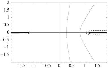
Figure 4: Integration path for Eq. (79) in the $y$-complex plane (thin solid lines) for $\nu_{3}\,H^{2}=0.3$ and ${\underline{\delta}\!s}/{\sigma_{s}}=0.3$ and $1$. The two half bold lines on the real axis represent the location singularities for $\varphi(y)$. For large values of $\phi$ the integration path is pushed along the singular part (dashed line).

The one-point probability distribution function is then given by the inverse Laplace transform of $\varphi(y)$

$$P({\underline{\delta}\!s})=\int_{-{\rm i}\infty}^{{\rm i}\infty}\frac{{\rm d}y}{2\pi\,{\rm i}\,{\sigma_{s}}^{2}}\exp\left[-\frac{\varphi(y)}{{\sigma_{s}}^{2}}+\frac{{\underline{\delta}\!s}\ y}{{\sigma_{s}}^{2}}\right],$$ (79)

where ${\sigma_{s}}$ is the variance of ${\underline{\delta}\!s}$. The global properties of $P({\underline{\delta}\!s})$ can be derived from the properties of the cumulant generating function.

From the expression (74) one can obtain the expression of $\tau$ in (77),

$$\tau(1-\nu_{3}\tau^{2}/3)^{3/2}=-y$$ (80)

from which the expression of $\varphi(y)$ can be explicitly computed. The properties of $\varphi(y)$ in the complex plane are going to depend on those of $\tau$.

The shape of the PDF can be calculated from a numerical integration in the complex plane. In practice to complete such a numerical integration one must choose an adequate path in the $y$ plane to make the integral convergent. This is achieved in imposing that the quantity in the exponent remains real along the trajectory which can be obtained if the trajectory crosses the real axis at the saddle point position, $y_{s}$, defined by

$$\frac{{\rm d}\varphi(y)}{{\rm d}y}|_{y=y_{s}}={\underline{\delta}\!s},$$ (81)

which with Eq. (78) is given by the value of $\tau_{s}$ for which ${\cal G}(\tau_{s})={\underline{\delta}\!s}$ and then $y_{s}=-\tau_{s}/{\cal G}^{\prime}(\tau_{s})$. Example of such integration path are presented on Fig. 4.

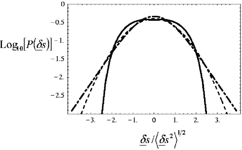
Figure 5: Shape of the one-point PDF of ${\underline{\delta}\!s}$ for $\nu_{3}\,H^{2}=0.3$ (dot-dashed line) or $\nu_{3}\,H^{2}=-0.3$ (solid line) compared to a Gaussian distribution (dashed line).

The resulting PDFs are shown on Fig. 5. They clearly exhibit non-Gaussian features (the Gaussian case is shown as a dashed line). The magnitude of these features depend on the value and sign of $\nu_{3}$, that is indeed related to the value and sign of the coupling constant $\lambda$. In the following we explore in some details the behavior of the PDF in different cases.

VI Properties of the isocurvature mode PDF

VI.1 The behavior of the PDF for small values of ${\underline{\delta}\!s}$

For small values of ${\underline{\delta}\!s}/{\sigma_{s}}$ it is possible to derive an explicit expression for the one-point PDF based on a saddle point approximation. In Eq. (79) one can expand $\varphi(y)$ around the saddle point defined previously, Eq. (81).

The resulting formal expression of the PDF then reads,

$$P({\underline{\delta}\!s}){\rm d}{\underline{\delta}\!s}={{\rm d}{\underline{\delta}\!s}\over\sqrt{2\pi\varphi^{\prime\prime}(y_{s})\,{\sigma_{s}}^{2}}}\,\exp\left[-{\tau^{2}\over 2{\sigma_{s}}^{2}}\right]$$ (82)

which can be calculated from the explicit expression of $\varphi$,

$$P({\underline{\delta}\!s}){\rm d}{\underline{\delta}\!s}=\sqrt{\frac{3}{2\,\pi}\left|\frac{1-{\underline{\delta}\!s}^{2}\nu_{3}}{(3+{\underline{\delta}\!s}^{2}\,\nu_{3})^{3}}\right|}\exp\left[-\frac{3\,{\underline{\delta}\!s}^{2}}{(6+2\,{\underline{\delta}\!s}^{2}\,\nu_{3}){\sigma_{s}}^{2}}\right]\frac{{\rm d}{\underline{\delta}\!s}}{{\sigma_{s}}}.$$ (83)

This result is valid as long as ${\underline{\delta}\!s}^{2}\,\nu_{3}$ is small compared to unity. For larger values of ${\underline{\delta}\!s}$ the behavior of the PDF depends crucially on the sign the $\lambda$.

This formula provides actually a very good description of the overall PDF shape when $\lambda$ is positive (since excursion to rare events are anyway not permitted).

VI.2 The rare event tails in case of negative $\lambda$

When $\nu_{3}$ is positive, that is when $\lambda$ is negative, the shape of the potential is such that it favors the rare event tails. The behavior of the probability distribution function in the rare event tails depends in particular on the analytic properties of $\varphi(y)$ in the complex plane. For positive values of $\nu_{3}$ it can be easily checked from Eq. (80) that $\tau(y)$, and consequently $\varphi(y)$ is non-analytic on the real axis with two symmetric singularities at finite distances of the origin,

$$\tau_{c}=\epsilon\,\frac{1}{2}\sqrt{\frac{3}{\nu_{3}}},$$ (84)

($\epsilon=\pm 1$) corresponding to values of $\tau$ where its derivative with respect to $y$ is diverging. In the vicinity of this point it is easy to expand first the expression of $y$ as a function of $\tau$,

$$y=\epsilon\,y_{c}+\epsilon\,\left(\tau-\tau_{c}\right)^{2}$$ (85)

with

$$y_{c}=-\frac{9}{16\sqrt{\nu_{3}}}$$ (86)

and then the expression of $\varphi(y)$ reads [taking advantage of Eq. 78]

$$\varphi(y)=\varphi_{c}+r_{c}\,(\epsilon\,y-y_{c})-a_{c}(\epsilon\,y-y_{c})^{3/2}+\dots$$ (87)

with

$$\varphi_{c} = -\frac{3}{16\nu_{3}}$$ (88)

$$a_{c} = \frac{1}{\sqrt{\nu_{3}}}$$ (89)

$$r_{c} = \frac{16}{9\sqrt{3}\,\nu_{3}^{1/4}}$$ (90)

Those singularities induce exponential tails in the PDF of ${\underline{\delta}\!s}$ (a very complete mathematical investigation of such cases can be found in [47]). The shape of the tails are of the form $\exp(-|{\underline{\delta}\!s}|/{\underline{\delta}\!s}_{c}/{\sigma_{s}}^{2})$ where ${\underline{\delta}\!s}_{c}$ is given by the inverse value of $y$ at the singularity, ${\underline{\delta}\!s}_{c}=16\sqrt{\nu_{3}}/9$.

To be more precise the expression (83) ceases to be valid for $|{\underline{\delta}\!s}|>{\underline{\delta}\!s}_{m}$ where ${\underline{\delta}\!s}_{m}\equiv{\cal G}(\tau_{c})$. For larger values of ${\underline{\delta}\!s}$ the saddle point position in $y$ is pushed towards one of the singularities, $\pm y_{c}$. The behavior of the PDF will then be dominated by the behavior of $\varphi(y)$ around this point, Eq. (87), in which a regular part $\varphi_{c}+r_{c}(\epsilon\,y-y_{c})$ and a singular part $a_{c}\,(\epsilon\,y-y_{c})^{3/2}$ appear. One can then make the integration path in $y$ in Eq. (79) running along the real axis (both ways) crossing it at $y=y_{c}$ so that it can be described by the real variable $u$ varying from 0 to $\infty$ with,

$$y=\epsilon\,y_{c}+\epsilon\,u\,e^{\pm{\rm i}\pi}$$ (91)

where the sign is changing according to whether $y$ is above or under the real axis. Expanding the singular part in the exponential one gets,

$$P({\underline{\delta}\!s})={a_{c}}\int_{0}^{\infty}\frac{{\rm d}u}{2\pi{\rm i}\,{\sigma_{s}}^{4}}\,u^{3/2}{e^{\pm 3{\rm i}\pi/2}}\exp\left[\frac{-\varphi_{c}+\epsilon\,y_{c}\,{\underline{\delta}\!s}-(\epsilon\,{\underline{\delta}\!s}-r_{c})u}{{\sigma_{s}}^{2}}\right].$$ (92)

The singular value in $y$ to consider (that is the value of $\epsilon$ in the previous equation) depends on the sign of ${\underline{\delta}\!s}$ (the positive tail corresponds to negative value of $y$) so that finally one gets,

$$P({\underline{\delta}\!s})={a_{c}\,{\sigma_{s}}\over\ \Gamma(-3/2)}\left({|{\underline{\delta}\!s}|-r_{c}}\right)^{-5/2}\exp\left(-\frac{{\varphi_{s}}+|y_{s}\,{{\underline{\delta}\!s}}|}{{\sigma_{s}}^{2}}\right).$$ (93)

which, for the parameters describing the singular behavior of $\varphi$, gives,

$$P({\underline{\delta}\!s})=\frac{4\,{\sigma_{s}}}{3\sqrt{3\pi}\,\nu_{3}^{1/4}}\,\left(|{\underline{\delta}\!s}|-\frac{1}{\sqrt{\nu_{3}}}\right)^{-5/2}\exp\left(\frac{3}{16\nu_{3}\,{\sigma_{s}}^{2}}-\left|\frac{9{\underline{\delta}\!s}}{16\sqrt{\nu_{3}}\,{\sigma_{s}}^{2}}\right|\right)$$ (94)

It is clear for this expression that the rare event tails are very different from a Gaussian distributed variable.

VI.3 Bounding values in case of a positive $\lambda$

When $\nu_{3}$ is negative, that is when $\lambda$ is positive, we are in the opposite case. We expect that the rare event tails to be chopped out. Actually in this case it is easy to see that there is no singularity on the real axis. It implies that the integration contour can be moved from the imaginary axis to the left or the right to an arbitrarily large distance. When $|y|\to\infty$, we have $\tau\sim|y|^{1/4}(-3/\nu_{3})^{3/8}$ which implies that,

$$\varphi(y)\sim-\left(\frac{3}{-\nu_{3}}\right)^{1/2}|y|$$ (95)

for large values of $y$. As a consequence for large enough values of $\phi$ the integral simply vanishes away. The values of $\phi$ are therefore are bounded by $\pm\sqrt{-3/\nu_{3}}$. The shape of the PDF near the bounding values can also be computed explicitly from the behavior of $\varphi$ for large values of $y$,

$$\varphi(y)=-\left(\frac{3}{-\nu_{3}}\right)^{1/2}|y|+\frac{3^{3/4}}{(-\nu_{3})^{3/4}}\sqrt{|y|}+\frac{9}{8\,\nu_{3}}\dots$$ (96)

Then the expression of the integral (79) reads,

$$P({\underline{\delta}\!s})=\int_{-{\rm i}\infty}^{+{\rm i}\infty}\frac{{\rm d}y}{2\pi{\rm i}\,{\sigma_{s}}^{2}}\exp\left[\frac{(\sqrt{-3/\nu_{3}}-|{\underline{\delta}\!s}|)\,|y|-a\,|y|^{1/2}-9/(8\nu_{3})}{{\sigma_{s}}^{2}}\right]$$ (97)

with

$$a=\frac{3^{3/4}}{(-\nu_{3})^{3/4}}.$$ (98)

A simple change of variable, $t^{1/2}=a\,y^{1/2}/{\sigma_{s}}^{2}$, shows that it can be written,

$$P({\underline{\delta}\!s})=\frac{{\sigma_{s}}^{2}}{a^{2}}\exp\left(-\frac{9}{8\nu_{3}{\sigma_{s}}^{2}}\right)\int_{-{\rm i}\infty}^{+{\rm i}\infty}{{\rm d}t\over 2\pi{\rm i}}\exp\left(-t^{1/2}+z\,t\right)$$ (99)

with

$$z={{\sigma_{s}}^{2}(\sqrt{-3/\nu_{3}}-|{\underline{\delta}\!s}|)\over a^{2}}$$ (100)

The behavior of the PDF near the bounding values are determined by the small values of $z$. The expression of the PDF can be obtained in this regime by a saddle point approximation, similar to Eq. (83), which leads to,

$$P({\underline{\delta}\!s})={{\sigma_{s}}^{2}\over a^{2}}{1\over 2\sqrt{\pi}}\,z^{-{3\over 2}}\,\exp\left[-{1\over 4\,z}-\frac{9}{8\nu_{3}{\sigma_{s}}^{2}}\right].$$ (101)

which reexpressed in terms of ${\underline{\delta}\!s}$ gives the behavior of the PDF near the bounds,

$$P({\underline{\delta}\!s})={1\over 2\sqrt{\pi}\,{\sigma_{s}}}\,\left(1-\frac{|{\underline{\delta}\!s}|}{\sqrt{-3/\nu_{3}}}\right)^{-{3\over 2}}\,\exp\left[-{9\over 8\nu_{3}\,{\sigma_{s}}^{2}}-{(-3/\nu_{3})^{3/2}\over 4\,{\sigma_{s}}^{2}(\sqrt{-3/\nu_{3}}-|{\underline{\delta}\!s}|)}\right].$$ (102)

The PDF is found to go continuously to zero at ${\underline{\delta}\!s}=\pm\sqrt{-3/\nu_{3}}$ positions.

VII Conclusions

In this paper we have explored the possibility of generating significant non-Gaussian initial metric perturbations in the context of inflationary cosmology while preserving a power spectrum of slow roll type adiabatic fluctuations. We found that the only viable mechanism is through a multiple field inflation where transverse (e.g. isocurvature) modes developed non Gaussian properties that can be subsequently transferred to the adiabatic fluctuations if the classical field trajectory is bent.

We have pointed out that quartic type coupling in the transverse modes is the most natural type of couplings for providing non-Gaussianities in the sense that in this case no fine-tuning in the value of the coupling constant has to be invoked. We stress that in the context of such a mechanism, unlike any others, the amount of non-Gaussianities that can be fuelled in the adiabatic fluctuations can be almost arbitrarily large.

We have examined in more details the case where the isocurvature mode generation (that is when they reach the Hubble size during the inflationary period) and the adiabatic-isocurvature mode mixing happen at very different time. The reason we consider this case is two-fold. First it is somewhat pedagogical since it shows that these two stages do not have to be concomitant. Second it implies that the non-Gaussian properties of the isocurvature modes developed mainly during the time they live at super-Hubble scales. It makes their computation much more simple since we can avoid a full treatment of the nonlinear field evolution at a quantum level (and it turns out that such a computation is not straightforward at all!). For modes living at super-Hubble scales we allowed ourselves to view the field evolution as the one of a classical stochastic field. In this case it is then possible to pursue the calculations to completion in the sense that it is possible to derive their whole set of correlation properties.

In particular we have been able to derive the one-point field cumulants at tree order in the weak coupling limit in a consistent way and finally build up the one-point probability distribution function of the field value. In such class of models, the statistical properties of the curvature perturbation are described by the superposition of a Gaussian and a non-Gaussian contributions with a relative weight proportional to the bending angle, $\Delta\theta$, of the trajectory in field space during slow-roll. The non-Gaussian component is fully characterized by a single parameter, $\nu_{3}$, related to the reduced fourth order connected cumulant and has the same variance as the Gaussian contribution. For practical purposes, we emphasize that its PDF is well approximated by Eq. (83) that reproduces accurately the numerically computed PDF within our approximation scheme. Thus, all the statistical properties can be encapsuled in two parameters. These results give some insights on what type of non-Gaussian features can appear in future large-scale structure or CMB surveys while assuming the inflationary prejudice. Note that the kind of non-Gaussianity described here departs from that generated by the non-linear gravitational dynamics, in particular it has no skewness. There is still however some ways between these results and their observational consequences. How non-Gaussian properties that are present at super-Hubble scales are transferred for instance to the CMB anisotropies at sub-Hubble scales is not totally straightforward. Whether such effects could be actually observed when observational aspects are taken into account demands in-depth analysis.

References

-
[1]
V. Mukhanov and G.V. Chibisov, JETP Lett. 33 (1981) 532;
S.W. Hawking, Phys. Lett. B 115 (1982) 295;
V.F. Mukhanov, H.A. Feldman, and R.H. Brandenberger, Phys. Rep. 215 (1992) 203.
A.D. Linde, Particle physics and inflationary cosmology, Harwood (Chur, Switzerland, 1990);
A.R. Liddle and D.H. Lyth, Cosmological inflation and large-scale structure, Cambridge University Press (Cambrige, UK, 2000). -
[2]
A.D. Linde, Phys. Lett. B 158 (1985) 375;
L.A. Kofman, Phys. Lett. B 173 (1986) 400. - [3] D. Polarski and A.A. Starobinsky, Phys. Rev. D 50 (1994) 6123.
- [4] J. García-Bellido and D. Wands, Phys. Rev. D 53 (1996) 5437.
- [5] V.F. Mukhanov and P.J. Steinhardt, Phys. Lett. B 422 (1998) 52.
- [6] D. Langlois, Phys. Rev. D 59 (1999) 123512.
- [7] C. Gordon, D. Wands, B.A. Basset, and R. Maartens, Phys. Rev. D 63 (2000) 023506.
- [8] J.H. Hwang and H. Noh, Phys. Lett. B 495 (2000) 277.
- [9] L. Kofman and D. Pogosyan, Phys. Lett. B 214 (1988) 548.
- [10] M. Bucher, K. Moodley, and N. Turok, astro-ph/0007360.
- [11] D. Langlois and A. Riazuelo, Phys. Rev. D 62 (2000) 043504.
- [12] M. Bucher, K. Moodley, and N. Turok, Phys. Rev. Lett. 87 (2001) 191301.
- [13] T.J. Allen, B. Grinstein, and M.B. Wise, Phys. Lett. B 197 (1987) 66.
-
[14]
L. Kofman, G.R. Blumenthal, H. Hodges, and J.R. Primack,
in “Large scale structures and peculiar motions in the universe”,
eds. D.W. Latham and L. da Costa (1989) 339;
I. Antoniadis, P.O. Mazur, and E. Motola, Phys. Rev. Lett. 79 (1997) 14;
P.J. E. Peebles, Astrophys. J. 483 L1;
R. Scoccimarro, astro-ph/0002037. -
[15]
E.J. Copeland, J.E. Lidsey, and D. Wands,
Phys. Lett. B 443 (1998) 97;
R. Durrer and M. Sakellariadou, Phys. Rev. D 62 (2000) 123504. - [16] M. Bucher and Y. Zhu, Phys. Rev. D 55 (1997) 7415.
-
[17]
A. Gangui and S. Mollerach, Phys. Rev. D 54 (1996) 4750;
R. Durrer, M. Kunz, and A. Melchiorri, Phys. Rep. 364 (2002);
L. Perivolaropoulos, hep-ph/9212228. -
[18]
J. Martin, A. Riazuelo, and M. Sakellariadou,
Phys. Rev. D 61 (2000) 083518;
A. Gangui, J. Martin, and M. Sakellariadou, astro-ph/0205202. -
[19]
J. Lesgourgues, D. Polarski, and A.A. Starobinsky,
Month. Not. R. Astron. Soc. 297 (1998) 769;
J. Lesgourgues, Nucl. Phys. B 582 (2000) 593;
A.A. Starobinsky, Grav. Cosmol. 4 (1998) 88. - [20] D.S. Salopek, Phys. Rev. D 45 (1992) 1139.
- [21] D.S. Salopek and J.R. Bond, Phys. Rev. D 42 (1990) 3936.
- [22] D. La and P.J. Steinhardt, Phys. Rev. Lett. 62 (1989) 376.
- [23] K. Yamamoto et al., Phys. Rev. D 46 (1992) 4206.
-
[24]
A. Linde and V.F. Mukhanov,
Phys. Rev. D 56 (1997) 535;
I. Antoniadis, P.O. Mazur, and E. Motola, astro-ph/9705200. - [25] N. Bartolo, S. Matarrese, and A. Riotto, Phys. Rev. D 64 (2001) 083514.
- [26] N. Bartolo, S. Matarrese, and A. Riotto, hep-ph/0112261.
- [27] H.B. Sanvik and J. Magueijo, astro-ph/0010395.
- [28] G. Rocha, J. Magueijo, M. Hobson, and A. Lasenby, Phys. Rev. D 64 (2001) 06352.
- [29] M.G. Santos et al., astro-ph/0107588.
- [30] F. Bernardeau, S. Colombi, E. Gaztañaga, and R. Scoccimaro, astro-ph/0112551.
- [31] R. Durrer, R. Juszkiewicz, M. Kunz, and J.-P. Uzan, Phys. Rev. D62 (2000) 021301(R).
- [32] F. Bernardeau, Y. Mellier, and L. van Waerbeke, astro-ph/0201029.
- [33] F. Bernardeau, Y. Mellier, and L. van Waerbeke, astro-ph/0201032.
- [34] S. Hawking and G.F.R. Ellis, Large scales structure of spacetime, Cambridge University Press (1973).
- [35] N.D. Birrell and P.C.W. Davies, Quantum fields in curved space, Cambridge University Press (1982).
-
[36]
A. Vilenkin and L.H. Ford, Phys. Rev. D 26 (1982) 1231;
A.D. Linde, Phys. Lett. B 116 (1982) 335;
A.A. Starobinsky, Phys. Lett. B 117 (1982) 175;
L.A. Kofman and A.D. Linde, Nuc. Phys. B 282 (1987) 555. - [37] N.C. Tsamis and R.D. Woodard, Class. Quant. Grav. 11 (1994) 2969.
- [38] L.H. Ford and L. Parker, Phys. Rev. D 16 (1977) 245.
- [39] B. Allen and A. Folacci, Phys. Rev. D 35 (1987) 3771.
- [40] B.S. de Witt, in Relativity, groups and topology II, Proceedings of Les Houches summer school 1983, edited by B.S. de Witt and R. Stora, (North Holland, Amsterdam, 1984).
- [41] L.H. Ford and C. Pathinayake, Phys. Rev. D 39 (1989) 3642.
- [42] A. Vilenkin and L.H. Ford, Phys. Rev. D 26 (1982) 1231.
- [43] K. Kirsten and J. Garriga Phys. Rev. D 48 (1993) 567.
- [44] A.J. Tolley and N. Turok, hep-th/0108119.
- [45] D. Polarski, Phys. Rev. D 41 (1990) 442; ibid., Phys. Rev. D 41 (1990) 2519; ibid., Phys. Rev. D 43 (1991) 1892.
-
[46]
A.A. Starobinsky, and J. Yokoyama, Phys. Rev. D 50 (1994) 6357;
P.J.E. Peebles and A. Vilenkin, Phys. Rev. D 60 (1999) 103506. - [47] R. Balian and R. Schaeffer, Astron. Astrophys. 220 (1989) 1.
- [48] D.H. Lyth and A. Riotto, Phys. Rep. 314 (1999) 1.