susypic curly_len2.5thick arrow_len3thick thin0.5thick dot_len1mm wiggly_len4thick style_def gluino expr p = cdraw (curly p); cdraw p enddef;

DESY 02-097 July 2002
PSI-PR-02-06

Testing coupling relations in
SUSY-QCD at a Linear Collider

A. Brandenburg ^a,, M. Maniatis ^a, M. M. Weber ^b

^a Deutsches Elektronen-Synchrotron DESY, 22603 Hamburg, Germany

^b Paul Scherrer Insitut PSI, CH-5232 Villigen, Switzerland

Abstract:
Supersymmetry predicts that gauge couplings are equal to the corresponding gaugino-sfermion-fermion Yukawa couplings. This prediction can be tested for the QCD sector of the MSSM by studying the processes $e^{+}e^{-}\to$ squark+antisquark+gluon and $e^{+}e^{-}\to$ squark+antiquark+gluino at a future linear collider. We present results for these processes at next-to-leading order in $\alpha_{s}$ in the framework of the MSSM. We find sizable SUSY-QCD corrections. The renormalization scale dependence is significantly reduced at next-to-leading order.

1 Introduction

Softly broken supersymmetry predicts that each known particle has a superpartner with equal gauge quantum numbers and spin different by $1/2$. Further, the gauge couplings have to be equal to the corresponding gaugino-sfermion-fermion Yukawa couplings. These coupling relations are vital for the cancellation of quadratic divergencies. Therefore, in order to establish supersymmetry experimentally, one not only has to find new particles and measure their quantum numbers, but also to verify the SUSY coupling relations. For the QCD sector of the MSSM, the coupling relation is depicted in Fig. 1. Analogous relations hold for the electroweak sector [1].

(0,0)(0,0) (2.5,3.0) i1 o2 gluon,tension=1.5i1,v1 fermiono1,v1,o2 $\bar{q}$o1 $q$o2 $g$i1

(0,0)(0,0) (2.5,3) i1 o2 gluon,tension=1.5i1,v1 scalaro1,v1,o2 $\bar{\tilde{q}}$o1 $\tilde{q}$o2 $g$i1

(0,0)(0,0) (2.5,3) i1 o2 gluino,tension=1.5i1,v1 scalaro1,v1 fermionv1,o2 $\bar{\tilde{q}}$o1 $q$o2 $\tilde{g}$i1

Gauge coupling $g_{s}$              $=$                Yukawa coupling $\hat{g}_{s}$

Figure 1: Coupling relation for the QCD sector of the MSSM.

The SU(3) coupling relation can be verified at $e^{+}e^{-}$ colliders by measuring the cross sections for the processes

$$e^{+}e^{-}\to q\bar{q}g\hskip 56.9055pt(a),$$

$$e^{+}e^{-}\to\tilde{q}\bar{\tilde{q}}g\hskip 56.9055pt(b),$$ (1)

$$e^{+}e^{-}\to q\bar{\tilde{q}}\tilde{g},\bar{q}\tilde{q}\tilde{g}\hskip 34.14322pt(c),$$

and compare them to precise theoretical predictions, i.e. to a calculation at next-to-leading order (NLO) in $\alpha_{s}$. The standard NLO QCD corrections to the 3-jet production process (1a) are well known [2]. Here we will also present the virtual SUSY-QCD corrections to order $\alpha_{s}^{2}$ for this process. Cross sections for processes (1b) and (1c) have been computed to leading order in [3]. We have recently performed a full NLO calculation for these processes. In this talk, we will discuss our main results. A detailed account of our work will be given elsewhere [4].

2 Squark and gluino production at leading order

We first discuss the leading order cross sections for processes (1b) and (1c). We allow only light quarks $q=u,d,s,c,b$ (and antiquarks) in the final state of process (1c) and neglect their masses. We further exclude scalar top quarks as final state particles. The mixing between the chiral components $\tilde{q}_{L}$ and $\tilde{q}_{R}$ is neglected and all five squark flavours are assumed to be mass degenerate. The cross section for (1b) diverges as the gluon energy goes to zero. We define an infrared finite cross section as follows:

$$\sigma(E_{\rm cut})\equiv\sum_{q=u,d,s,c,b}\ \sum_{h=L,R}\sigma(e^{+}e^{-}\to\tilde{q}_{h}\bar{\tilde{q}}_{h}X;\ E_{X}>E_{\rm cut}),$$ (2)

where $X=g$ at leading order. The minimal energy $E_{\rm cut}$ can be chosen by the experimentalist. We will take $E_{\rm cut}=50$ GeV for most of the numerical results below. For process (1c), the total cross section is defined by

$$\sigma_{\rm tot}\equiv\sum_{q=u,d,s,c,b}\ \sum_{h=L,R}\Big{\{}\sigma(e^{+}e^{-}\to\tilde{q}_{h}\bar{q}\tilde{g})+\sigma(e^{+}e^{-}\to q\bar{\tilde{q}}_{h}\tilde{g})\Big{\}}.$$ (3)

Figs. 2a and 2b show the leading order cross sections $\sigma(E_{\rm cut})$ and $\sigma_{\rm tot}$ defined above. We also plot for comparison the LO cross section for $e^{+}e^{-}\to\tilde{q}\bar{\tilde{q}}$. We distinguish between the cases $m_{\tilde{q}}<m_{\tilde{g}}$ (Fig. 2a) and $m_{\tilde{q}}>m_{\tilde{g}}$ (Fig. 2b). One sees that even for rather large squark and gluino masses, the cross section $\sigma(E_{\rm cut})$ defined in (2) reaches values of several tens of femtobarn, while the cross section $\sigma_{\rm tot}$ defined in (3) is about one order of magnitude smaller.

Figure 2: Leading order cross sections for squark and gluino production in $e^{+}e^{-}$ collisions for $m_{\tilde{g}}>m_{\tilde{q}}$ (a) and $m_{\tilde{g}}>m_{\tilde{q}}$ (b).

3 SUSY-QCD corrections to $e^{+}e^{-}\to\tilde{q}\bar{\tilde{q}}g$ and $e^{+}e^{-}\to q\bar{\tilde{q}}\tilde{g}/\bar{q}\tilde{q}\tilde{g}$

The calculation of the NLO SUSY-QCD corrections to processes (1b) and (1c) requires the evaluation of both virtual and real corrections. Possible real corrections at order $\alpha_{s}^{2}$ to process (1b) are contributions from the processes $e^{+}e^{-}\to\tilde{q}\bar{\tilde{q}}gg$ and $e^{+}e^{-}\to\tilde{q}\bar{\tilde{q}}q\bar{q}$, while the real corrections to process (1c) consist of real gluon emission, $e^{+}e^{-}\to q\bar{\tilde{q}}\tilde{g}g$ . Sample Feynman diagrams for both virtual and real corrections are shown in Figs. 3a-3d.

(0,0)(0,0) (5,4) i1 o3 photon,tension=4,label=$\gamma$,,$Z^{0}$,label.sid=righti1,v1 phantom,tension=1v1,v2 phantomv2,o1 phantom,tension=1v1,v4 phantomv4,o3 phantom,tension=0.6v1,v3 phantomv3,o2 fermionv4,v1,v2 gluinov2,v3,v4 scalarv2,o1 scalaro3,v4 gluonv3,o2 $g$o2 $\tilde{q}$o1 ${\bar{\tilde{q}}}$o3	(0,0)(0.66,0) (5,4) i1 o4 photon,tension=3,label=$\gamma$,,$Z^{0}$,label.sid=righti1,v1 scalaro1,v1 scalarv1,o4 gluonv1,v2,o3 $g$o3 gluonv2,o2 $g$o2 $\tilde{q}$o4 $\bar{\tilde{q}}$o1	(0,0)(1.33,0) (5,4) i1 o3 photon,tension=4,label=$\gamma$,,$Z^{0}$,label.sid=righti1,v1 phantom,tension=1v1,v2 phantomv2,o1 phantom,tension=1v1,v4 phantomv4,o3 phantom,tension=.6v1,v3 phantomv3,o2 scalaro1,v2,v1 scalarv1,v4 quarkv4,v3,o2 gluonv2,v3 gluinov4,o3 $q$o2 $\tilde{g}$o3 $\bar{\tilde{q}}$o1	(0,0)(0.66,0) (5,4) i1 o4 photon,tension=3,label=$\gamma$,,$Z^{0}$,label.sid=righti1,v1 phantomo1,v1 phantomv1,o4 scalaro1,v3,v1 scalarv1,v2 quarkv2,o4 gluinov2,o3 gluonv3,o2 $\tilde{g}$o3 $g$o2 $q$o4 $\bar{\tilde{q}}$o1
(a)	(b)	(c)	(d)

Figure 3: Sample Feynman diagrams for virtual and real corrections to $e^{+}e^{-}\to\tilde{q}\bar{\tilde{q}}g$ (Figs.  (a) and (b)), and to $e^{+}e^{-}\to q\bar{\tilde{q}}\tilde{g}$ (Figs.  (c) and (d)). The trivial leptonic part is not shown.

In the calculation of the virtual corrections one encounters both ultraviolet and soft and collinear divergencies. For convenience, we regularize them by using conventional dimensional regularization (DREG). As is well known, DREG violates supersymmetry. In particular, SUSY-invariant physical quantities involving the gauge and Yukawa couplings $g_{s}$ and $\hat{g}_{s}$ deviate by a finite amount in the exact SUSY limit. A SUSY-restoring counterterm can be derived from the Slavnov-Taylor identities [5]. This amounts to the following replacement of the Yukawa coupling $\hat{g}_{s}$ in the gluino-quark-squark vertex [6]:

$$\hat{g}_{s}=g_{s}\left[1+\frac{\alpha_{s}}{3\pi}\right].$$ (4)

The ultraviolet divergencies are removed by renormalization of the masses and the coupling. For the mass renormalization we use the on-shell scheme, while the strong coupling is renormalized in the $\overline{\rm MS}$ scheme. After renormalization the virtual corrections still contain soft and collinear singularities which manifest themselves in double and single poles in $\epsilon=(d-4)/2$. They are cancelled by singular contributions from the four parton final states which are due to soft gluons and collinear massless partons. These contributions have to be computed analytically in $d$ dimensions to perform the cancellation. For process (1b) we used the so-called dipole subtraction method [7], which has been recently generalized to include massive partons [8]. For process (1c) we used a variant of the phase space slicing method [9].

Figure 4: Cross section for $e^{+}e^{-}\to\tilde{q}\bar{\tilde{q}}X$ at leading order (dashed line) and including the SUSY-QCD corrections (full line) for $m_{\tilde{g}}=400$ GeV, $m_{\tilde{q}}=300$ GeV, $E_{\rm cut}=50$ GeV and $\mu=1$ TeV.

Figure 5: In (a), the dependence of $\sigma(E_{\rm cut})$ on the renormalization scale is shown, where the reference scale is $\mu_{0}=1$ TeV. In (b), the dependence on $E_{\rm cut}$ is depicted for $\mu=1$ TeV. The c.m. energy was fixed to be $\sqrt{s}=2$ TeV, and masses were chosen as in Fig. 4.

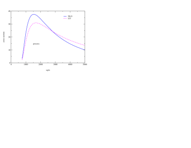
We now discuss our numerical results for the SUSY-QCD corrections, first for the process $e^{+}e^{-}\to\tilde{q}\bar{\tilde{q}}g$. Fig. 4 shows the cross section $\sigma(E_{\rm cut})$ defined in Eq. (2), where at NLO the unspecified part of the final state $X$ can be a single gluon, two gluons or a massless $q\bar{q}$ pair. In all cases we require $E_{X}>E_{\rm cut}$ and take in Fig. 4 $E_{\rm cut}=50$ GeV. For the masses we choose $m_{\tilde{g}}=400$ GeV and $m_{\tilde{q}}=300$ GeV. The renormalization scale is set to $\mu=1$ TeV. Fig. 4 shows that the SUSY-QCD corrections enhance the cross section in the peak region by about 20%.

In Fig. 5a we show the dependence of $\sigma(E_{\rm cut})$ on the renormalization scale $\mu$ for fixed $\sqrt{s}=2$ TeV and two different values for $E_{\rm cut}$. The $\mu$-dependence is significantly reduced by the inclusion of the order $\alpha_{s}^{2}$ corrections, thus leading to a more reliable theoretical prediction of the cross section. Fig. 5b shows the dependence of $\sigma(E_{\rm cut})$ on the cut parameter. We emphasize again that $E_{\rm cut}$ is a physical parameter that can be chosen by the experimentalist.

The inclusive cross section at LO and NLO for $e^{+}e^{-}\to q\bar{\tilde{q}}\tilde{g}/\bar{q}\tilde{q}\tilde{g}$ defined in (3) is shown in Fig. 6a and 6b for the cases $m_{\tilde{q}}<m_{\tilde{g}}$ and $m_{\tilde{q}}>m_{\tilde{g}}$, respectively. The cross section $\sigma_{\rm tot}$ reaches values up to 5 fb for the case $m_{\tilde{q}}=300$ GeV and $m_{\tilde{g}}=400$ GeV. The SUSY-QCD corrections enhance the cross section in the peak region by about 25%. For $m_{\tilde{q}}>m_{\tilde{g}}$, the cross section is below 1 fb, and this case is probably of no phenomenological interest. The NLO corrections reach values up to 80%.

Figure 6: Total cross section for gluino production in LO and NLO for $m_{\tilde{q}}<m_{\tilde{g}}$ (a) and $m_{\tilde{q}}>m_{\tilde{g}}$ (b).

Figure 7: Scale dependence of $\sigma_{\rm tot}$ in LO and NLO for the cases $m_{\tilde{q}}<m_{\tilde{g}}$ (a) and $m_{\tilde{q}}>m_{\tilde{g}}$ (b). The reference scale is $\mu_{0}=m_{\tilde{q}}+m_{\tilde{g}}$ in both cases.

The scale dependence of $\sigma_{\rm tot}$ is shown in Figs. 7a and 7b. For the phenomenologically more interesting case $m_{\tilde{q}}<m_{\tilde{g}}$ the inclusion of the SUSY-QCD corrections significantly reduces the theoretical uncertainty due to the arbitrariness of the scale choice.

4 SUSY-QCD corrections to $e^{+}e^{-}\to q\bar{q}g$

Finally we study the impact of SUSY-QCD corrections on the production of 3 jets. For this we have to compute the SUSY-QCD loop corrections to the process $e^{+}e^{-}\to q\bar{q}g$. The 3-jet cross section is defined as follows:

$$\sigma_{3}(y_{\rm cut})=\sigma(e^{+}e^{-}\to 3{\rm\ jets};y_{ij}>y_{\rm cut}),$$ (5)

where we take $y_{ij}=(p_{i}+p_{j})^{2}/s$ with $p_{i}$ denoting the four momenta of the final state partons. The cross section may be expanded as follows:

$$\sigma_{3}(y_{\rm cut})=\frac{\alpha_{s}}{2\pi}\sigma_{3}^{0}+\left(\frac{\alpha_{s}}{2\pi}\right)^{2}\left[\sigma_{3}^{1,\rm SUSY}+\sigma_{3}^{1,\rm QCD}\right]+O\left(\alpha_{s}^{3}\right).$$ (6)

Here $\sigma_{3}^{1,\rm QCD}$ denotes the ordinary QCD correction at order $\alpha_{s}^{2}$. The ‘genuine’ SUSY-QCD corrections are defined by

$$\Delta_{\rm SUSY}\equiv\frac{\alpha_{s}}{2\pi}\frac{\sigma_{3}^{1,\rm SUSY}}{\sigma_{3}^{0}}.$$ (7)

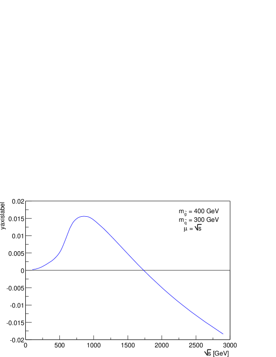
The dependence of $\Delta_{\rm SUSY}$ on $y_{\rm cut}$ turns out to be very small. We choose $y_{\rm cut}=(50{\rm\ GeV})^{2}/s$ and plot in Fig. 8 $\Delta_{\rm SUSY}$ as a function of $\sqrt{s}$ for $m_{\tilde{q}}=300$ GeV and $m_{\tilde{g}}=400$ GeV. Here we have used a decoupling scheme for the strong coupling, i.e. only the light quark flavours contribute to the running of $\alpha_{s}$. This ensures that $\Delta_{\rm SUSY}\to 0$ as the squark and gluino masses become large compared to the c.m. energy. Fig. 8 shows that the virtual SUSY-QCD corrections are tiny at the $Z$-pole, reach a maximum of about 1.5% around $\sqrt{s}=1$ TeV and eventually turn negative for large c.m. energies.

Figure 8: Impact of virtual SUSY-QCD corrections on the 3-jet cross section. We require $(p_{i}+p_{j})^{2}>(50\ {\rm GeV})^{2}$ for each pair $(i,j)$ of the final state partons.

5 Conclusions

The experimental verification of supersymmetric coupling relations is necessary to establish supersymmetry. The SU(3) coupling relation can be tested in $e^{+}e^{-}$ collisions by comparing measurements of the processes $e^{+}e^{-}\to q\bar{q}g,\ \tilde{q}\bar{\tilde{q}}g,\ q\bar{\tilde{q}}\tilde{g}/\bar{q}\tilde{q}\tilde{g}$ to precise, i.e. NLO calculations. We have computed the previously unknown order $\alpha_{s}^{2}$ SUSY-QCD corrections to the above processes. The corrections enhance the LO cross sections for $e^{+}e^{-}\to\tilde{q}\bar{\tilde{q}}g,\ q\bar{\tilde{q}}\tilde{g}/\bar{q}\tilde{q}\tilde{g}$ by about 20% or more in the peak region. The renormalization scale dependence is reduced for the cases of phenomenological interest.

References

- [1] J. L. Feng, H. Murayama, M. E. Peskin, X. Tata, Phys. Rev. D 52 (1995) 1418 [hep-ph/9502260]; M. M. Nojiri, K. Fujii, T. Tsukamoto, Phys. Rev. D 54 (1996) 6756 [hep-ph/9606370]. See also the talk by A. Freitas at this conference.
- [2] R. K. Ellis, D. A. Ross, A. E. Terrano, Nucl. Phys. B 178 (1981) 421; K. Fabricius, I. Schmitt, G. Kramer, G. Schierholz, Z. Phys. C 11 (1981) 315; J. A. Vermaseren, K. J. Gaemers, S. J. Oldham, Nucl. Phys. B 187 (1981) 301; Z. Kunszt, Phys. Lett. B 99 (1981) 429.
- [3] D. H. Schiller, D. Wähner, Nucl. Phys. B 259 (1985) 597.
- [4] A. Brandenburg, M. Maniatis, M. Weber, P. M. Zerwas, in preparation.
- [5] W. Hollik, D. Stöckinger, Eur. Phys. J. C 20 (2001) 105 [hep-ph/0103009].
- [6] S. P. Martin, M. T. Vaughn, Phys. Lett. B 318 (1993) 331 [hep-ph/9308222]; W. Beenakker, R. Höpker, P. M. Zerwas, Phys. Lett. B 378 (1996) 159 [hep-ph/9602378].
- [7] S. Catani, M. H. Seymour, Nucl. Phys. B 485 (1997) 291 [hep-ph/9605323]; Erratum-ibid. B510 (1997) 503.
- [8] S. Catani, S. Dittmaier, M. H. Seymour, Z. Trocsanyi, Nucl. Phys. B 627 (2002) 189 [hep-ph/0201036].
- [9] W. T. Giele, E. W. N. Glover, Phys. Rev. D 46 (1992) 1980.