On the Behaviour and Stability of Superconducting Currents

Abstract

: We present analytic and numerical results for the evolution of currents on superconducting strings in the classical $U(1)\times U(1)$ model. We derive an energy functional for the currents and charges on these strings, establishing rigorously that minima should exist in this model for loops of finite size (vortons) if both charge and current are present on the worldsheet. We then study the stability of the currents on these strings, and we find an analytic criterion for the onset of instability (in the neutral limit). This limit specifies a lower maximal current than previous heuristic estimates. We conclude with a discussion of the evolution of loops towards their final vorton state in the model under consideration.

and

PACS: 98.80.-k, 74.60.Jg

SLAC: hep-ph/0207199

1 Introduction

Topological defects are a class of exact solutions in field theories whose stability is enforced by topological reasons. In particular, strings, the class of defects associated with a non-trivial first homotopy group of the vacuum manifold, have been widely studied, since they seem to appear in a variety of generalisations of the Standard Model (GUTs, SUSY etc.). They are for example associated with the spontaneous symmetry breakdown of a $U(1)$ symmetry, like the axion or baryon symmetry (global), or electromagnetism (local) in superconductivity. Strings could therefore appear during a cosmological phase transition, and are prime candidates for a number of astrophysical puzzles, like the dark matter of the universe or the origin of the most energetic cosmic rays (for a review of cosmic defects, see ref. [1]).

In this paper, we shall be interested in a class of defects where the string’s field is coupled to another scalar field, which allows the build up of charge and currents on the worldsheet. Because of the non-dissipative properties of the currents on these strings, they are called superconducting.

The plan of this paper is as follows: in the next section, we will discuss the Lagrangian under consideration, and show how the amount of charge and currents is limited; in the following part, we will carry out an analysis of the energy functional of the condensate, to get a very simple analytic expression for it. We will then use our results to discuss the possibility of forming stable loops of superconducting strings. Finally, we will study the stability of currents on the string’s worldsheet and derive an exact analytic result for the onset of instability, which we shall illustrate by numerical simulations obtained from our full 3D field theory code.

2 The field theory model

The model under consideration here is the original $U(1)\times U(1)$ model, first proposed by Witten [2], and based on the Lagrangian

$$\mathcal{L} =(\partial_{\mu}\phi)(\partial^{\mu}\phi)^{+}+(\partial_{\mu}\sigma)(\partial^{\mu}\sigma)^{+}-\frac{\lambda_{\phi}}{4}(|\phi|^{2}-\eta_{\phi}^{2})^{2}$$ (1)

$$\leavevmode\nobreak\ \leavevmode\nobreak\ \leavevmode\nobreak\ \leavevmode\nobreak\ \leavevmode\nobreak\ \leavevmode\nobreak\ \leavevmode\nobreak\ \leavevmode\nobreak\ \leavevmode\nobreak\ \leavevmode\nobreak\ -\frac{\lambda_{\sigma}}{4}(|\sigma|^{2}-\eta_{\sigma}^{2})^{2}-\beta|\phi|^{2}|\sigma|^{2}\,.$$

where $\phi$ and $\sigma$ are complex scalar fields and $\lambda_{\phi},\,\lambda_{\sigma},\,\eta_{\phi},\,\eta_{\sigma}$ and $\beta$ are positive constants. We can arrange the parameters in this model such that the ground state has the $\phi$-symmetry broken ($|\phi|=\eta_{\phi}\neq 0$), while $\sigma$ remains symmetric $(|\sigma|=0)$. Under these circumstances, vortex solutions exist in the $\phi$-field. Here, we shall assume we have a vortex-string lying along the $z$-axis; in azimuthal coordinates, this solution takes the form,

$$\phi(r,\theta,z)=|\phi|(r)e^{i\theta}\,,$$ (2)

with $|\phi|(0)=0$ at the vortex centre and $|\phi|\rightarrow\eta_{\phi}$ as $r\rightarrow\infty$.

We wish to consider the conditions under which a condensate in the $\sigma$-field can emerge in the core of the string. This condensate can also carry currents and charges along the string, so we will represent it by the following ansatz which describes the dependence of these excitations on $z$ and $t$:

$$\sigma=|\sigma|(r)\exp^{i(\omega t+kz)},$$ (3)

We can see that the presence of charge and current causes a change in the Lagrangian $\delta\mathcal{L}=(\omega^{2}-k^{2})|\sigma|^{2}$, which alters the mass term [3, 4], and the vacuum expectation value of $\sigma$; indeed, we can rewrite the Mexican hat potential for $|\sigma|$ as:

$$V_{\sigma}=\frac{\lambda_{\sigma}}{4}\left[|\sigma|^{2}-\left(\eta_{\sigma}^{2}+\frac{2}{\lambda_{\sigma}}(\omega^{2}-k^{2})\right)\right]^{2}.$$ (4)

From the expression (4), we see that the $\phi$-symmetry will remain broken in the vacuum, with $|\phi|=\eta_{\phi}$, as long as we satisfy

$$\lambda_{\phi}\eta_{\phi}^{4}>\lambda_{\sigma}\left(\eta_{\sigma}^{2}+\frac{2(\omega^{2}-k^{2})}{\lambda_{\sigma}}\right)^{2},$$ (5)

If we want the $\sigma$-symmetry to be remain unbroken in the ground state ($|\sigma|=0$), then we need to ensure that the mass term for $\sigma$ is positive at infinity, that is,

$$m_{\sigma}^{2}\equiv\beta\eta_{\phi}^{2}-\frac{1}{2}\lambda_{\sigma}\eta_{\sigma}^{2}-\omega^{2}+k^{2}>0\,.$$ (6)

Now at the centre of the string we have $|\phi|=0$, so this mass term can become negative and $\sigma$ can develop a non-vanishing expectation value, provided that

$$\frac{1}{2}\lambda_{\sigma}\eta_{\sigma}^{2}+\omega^{2}-k^{2}>0\,.$$ (7)

However, the condition (7) is not sufficient to obtain a $\sigma$-condensate within the string, since we also have to consider its gradient energy cost. To determine this we follow the analysis of Haws et al. [5] and study the stability of the trivial solution $\sigma=0$ with perturbations of the form $\sigma=|\sigma(x,y)|e^{i\nu t}$, with $|\sigma|<<1$. The field equation, using the modified Mexican Hat potential (4), then becomes

$$-\partial_{r}\partial^{r}\sigma-\left(\frac{1}{2}\lambda_{\sigma}[\eta_{\sigma}^{2}+\frac{2(\omega^{2}-k^{2})}{\lambda_{\sigma}}]-\beta\lambda_{\phi}\eta_{\phi}^{4}r^{2}\right)\sigma=\nu^{2}\sigma\,,$$ (8)

which is an eigenvalue equation with a harmonic oscillator-like potential. Hence, we know the value of the ground state eigenvalue $\nu_{0}$, and we see that the trivial solution will be unstable for $\nu_{0}^{2}<0$ or, equivalently,

$$k^{2}-\omega^{2}<\frac{1}{2}\lambda_{\sigma}\eta_{\sigma}^{2}-\sqrt{\beta\lambda_{\phi}}\eta_{\phi}^{2}\,.$$ (9)

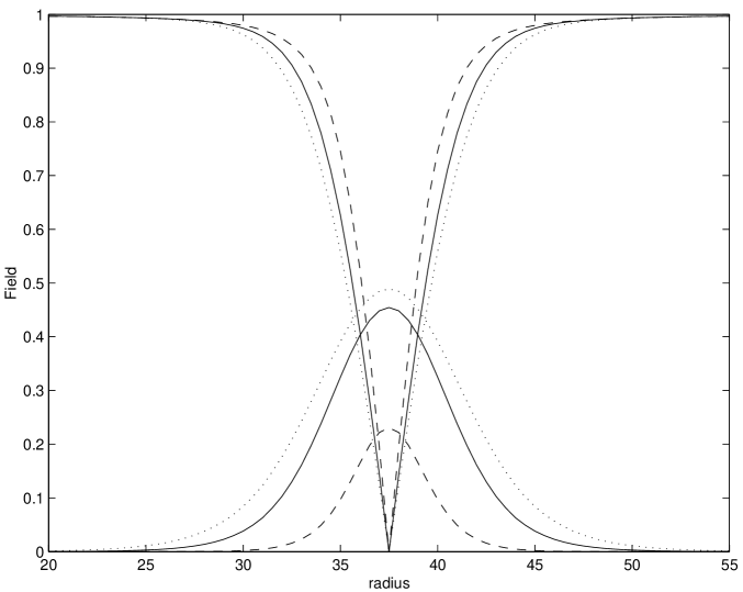
Figure 1: Profiles of the vortex and the condensate fields, with no charge and current (solid lines). The effects of adding a significant current (dashed) or charge density (dotted) is also illustrated; the (anti-)quenching effect of current (charge) is clear.

If (5), (6), and (9) are satisfied, $\sigma$ will form a condensate of width $\delta_{\sigma}\simeq m_{\sigma}^{-1}$, with two conserved quantities, the usual Noether charge $Q$ and a topological charge $N$, where:

$$Q=\omega\int dz\int dS\,|\sigma|^{2}\,,\qquad\qquad N=\int dz\,\frac{k}{2\pi}\,,$$ (10)

and a current flowing along the $z$ direction:

$$J_{z}=k\int dz\int dS\,|\sigma|^{2}\,.$$ (11)

The field configuration for a vortex with a condensate can be seen in fig. 1, with the influence of $k$ and $\omega$ also shown.

To conclude this section, we note that in the bare case ($\omega=k=0$), (5), (6), and (9) lead to the following inequalities on the parameters of the theory:

$$\beta<\frac{\lambda_{\sigma}}{4}\,,\qquad 2\eta_{\sigma}^{2}<\eta_{\phi}^{2}\,.$$ (12)

These equations will prove to be useful in the rest of the paper.

3 The energy functional

Starting from the Lagrangian (1), we can easily switch to a Hamiltonian formalism. In particular, we will be interested in the following in the energy of the condensate, which can be written in the form:

$$\mathcal{E}_{\sigma}=\int dz\int dS\left(|\nabla_{r}\sigma|^{2}+(k^{2}+\omega^{2})|\sigma|^{2}+(\beta|\phi|^{2}-\frac{1}{2}\lambda_{\sigma}\eta_{\sigma}^{2})|\sigma|^{2}+\frac{\lambda_{\sigma}}{4}|\sigma|^{4}\right)\,.$$ (13)

This is a rather complicated expression, so in order to simplify it we consider the equation of motion for $\sigma$:

$$-\partial_{r}\partial^{r}\sigma+(k^{2}-\omega^{2})\sigma+(\beta|\phi|^{2}-\frac{1}{2}\lambda_{\sigma}\eta_{\sigma}^{2})\sigma+\frac{\lambda_{\sigma}}{2}|\sigma|^{2}\sigma=0\,.$$ (14)

Multiplying (14) by the complex conjugate $\sigma^{+}$, integrating by parts, and then inserting the result in (13), we find:

$$\mathcal{E}_{\sigma}=-\frac{\lambda_{\sigma}}{4}\int d^{3}r\,|\sigma|^{4}+2\int d^{3}r\,\omega^{2}|\sigma|^{2}\,.$$ (15)

(It is easy to generalise this equation to the gauged case, making the obvious replacement $\omega\to\omega-A_{t}$.)

Now, if we recall the expression for the conserved charge $Q$ (10), we can rewrite the energy as:

$$\mathcal{E}_{\sigma}=-\frac{\lambda_{\sigma}}{4}\int d^{3}r|\sigma|^{4}+\frac{2Q^{2}}{\int d^{3}r\,|\sigma|^{2}}\,.$$ (16)

This equation (16) is interesting because it expresses the energy in the condensate as a function of conserved quantities, and of the two integrated moments $\Sigma_{2}$ and $\Sigma_{4}$, where

$$\Sigma_{n}=\int dS\,|\sigma|^{n}\,.$$ (17)

Note that $d\Sigma_{n}/dz=0$ with the ansatz (3), and so we can carry out the $z$-integration in (16) for a segment of finite length $L$ to obtain

$$\mathcal{E}_{\sigma}=-\frac{\lambda_{\sigma}}{4}\Sigma_{4}L+\frac{2Q^{2}}{\Sigma_{2}L}\,,$$ (18)

which is a purely analytic expression.

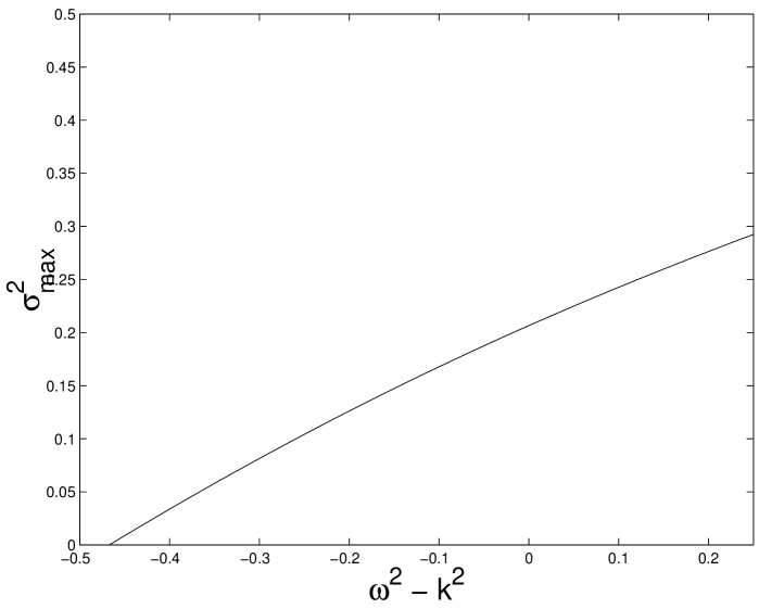
Figure 2: Plot of the numerical values for $\sigma_{\rm max}^{2}$, as a function of $\omega^{2}-n^{2}$.

This is the form of the energy functional we sought. All that is now required is to find an ansatz for the $\Sigma_{n}$, which can be done by noticing that:

$$\Sigma_{n}=\int dS\,|\sigma|^{n}\leavevmode\nobreak\ \leavevmode\nobreak\ \simeq\leavevmode\nobreak\ \leavevmode\nobreak\ \sigma_{\rm max}^{n}\times\delta_{\sigma}^{2}\leavevmode\nobreak\ \leavevmode\nobreak\ \simeq\leavevmode\nobreak\ \leavevmode\nobreak\ \frac{\sigma_{\rm max}^{n}}{m_{\sigma}^{2}}\,,$$ (19)

where $\delta_{\sigma}$ is the average width of the condensate, and $\sigma_{\rm max}$ is its maximum height in the vortex core. Now, we have the mass given by

$$m_{\sigma}^{2}=\beta\eta_{\phi}^{2}-\frac{1}{2}\lambda_{\sigma}\eta_{\sigma}^{2}-\omega^{2}+k^{2}\equiv\omega_{c}^{2}-\omega^{2}+k^{2}\,,$$ (20)

and we can see from fig. 2 that, up to a very good approximation, we can take

$$\sigma_{\rm max}^{2}\equiv\sigma_{0}(k_{c}^{2}-k^{2}+\omega^{2})\,,$$ (21)

where $k_{c}^{2}\simeq\frac{1}{2}\lambda_{\sigma}\eta_{\sigma}^{2}-\sqrt{\beta\lambda_{\phi}}\eta_{\phi}^{2}$ is the critical winding number density at which the condensate must vanish (obtained from (9)). (We note that in the gauged case, the picture is qualitatively the same, but that the gauge fields maintain the condensate against the quenching effect of the current; the height is then nearly constant in a somewhat wider range of $\omega^{2}-k^{2}$. Ultimately, however, $k_{c}^{2}$ is the same for both gauged and global cases.) If we further assume that $k_{c}\simeq\omega_{c}\simeq m_{o}$, we can factorize it out in (19) to yield:

$$\Sigma_{n}=\Sigma_{no}\frac{(1+v)^{\frac{n}{2}}}{1-v}\,,$$ (22)

with $v=(\omega^{2}-k^{2})/{m_{o}^{2}}$ and $\Sigma_{no}=\Sigma_{n}(\omega^{2}-k^{2}=0)$ is the value of $\Sigma_{n}$ in the so-called chiral case ($\omega=\pm k$). In particular, for $n=2$ this reduces to:

$$\Sigma\leavevmode\nobreak\ \equiv\leavevmode\nobreak\ \Sigma_{2}\leavevmode\nobreak\ =\leavevmode\nobreak\ \Sigma_{o}\,\frac{m_{o}^{2}+(\omega^{2}-k^{2})}{m_{o}^{2}-(\omega^{2}-k^{2})}\,.$$ (23)

As can be seen from fig. 3, the agreement between the numerical calculation and our analytic estimate (22) is remarkably good.

Figure 3: Plots of the numerical values for $\Sigma_{2}$ and $\Sigma_{4}$ (plain), and their analytic estimates (dashed) from (22).

4 The behaviour of superconducting loops

Cosmic strings tend to intercommute, and therefore we can expect the copious production of loops from a network of strings. Superconducting strings follow the same behaviour [6], but this time the charge and current due to the additional structure may prevent the shrinkage of the loop and stabilise the configuration [4]. These stable loops or vortons, effectively held up by their angular momentum, have been the subject of numerous studies (see, for example, refs. [7, 8, 9, 10, 11]).

Using the results of the previous sections, we would like to study the behaviour of these loops, starting from our analytic result for the energy of the condensate (18). However, we must also include the energy in the vortex, which we will model by $\mathcal{E}_{\phi}=\mu L$, where $\mu\sim\mathcal{O}(\eta_{\phi}^{2})$ is the mass per unit length of the string. We can then write our energy functional for the loop as

$$\mathcal{E}=\mu L-\frac{\lambda_{\sigma}}{4}\Sigma_{4}L+\frac{2Q^{2}}{\Sigma_{2}L}\,.$$ (24)

We will now discuss the various possible regimes for the charges and currents on these loops:

The chiral case, $\omega^{2}=k^{2}$:

We will first consider this limit, where $\omega^{2}-k^{2}=0$ (see refs. [12, 13] for a study of chiral loops using the 2D approach of [10]). In this regime, we always have $\Sigma=\Sigma_{o}$ and $\Sigma_{4}=\Sigma_{4o}$. Since these values remain fixed as the loop shrinks, it is easy to vary (24) to see that it will have a minimum for

$$L^{2}=\frac{2Q^{2}}{\Sigma_{o}(\mu-\frac{\lambda_{\sigma}}{4}\Sigma_{40})}=\frac{2N^{2}\Sigma_{o}}{(\mu-\frac{\lambda_{\sigma}}{4}\Sigma_{40})}\,.$$ (25)

Hence, the loop will contract (or expand) until $\omega^{2}=k^{2}={(\mu-\frac{1}{4}\lambda_{\sigma}\Sigma_{4o})}/({2\Sigma_{o}})$.

For this to be well defined, we should verify that $\mathcal{E}_{k=\omega=0}=\mu-\frac{\lambda_{\sigma}}{4}\Sigma_{4o}$ is positive. To do so, we note that this is the total energy in the bare superconducting string, and that the profiles $|\phi|(r)$ and $|\sigma|(r)$ minimise the value of this functional. By considering $\phi(\lambda r)$ and $\sigma(\lambda r)$, differentiating the field energy functional (13) with respect to $\lambda$ and setting this quantity to $0$ at $\lambda=1$, we obtain the result:

$$\mathcal{E}_{k=\omega=0}=\int d^{3}r(|\nabla\phi|^{2}+|\nabla\sigma|^{2})>0\,.$$ (26)

This ensures that the loop length $L^{2}$ is indeed well defined and that chiral loops must have a stable minimum of their energy. (Of course, we assume here that chiral currents are long-lived and that the final stable loop size is significantly larger than the vortex width.)

The electric and magnetic cases, $\omega^{2}-k^{2}\not=0$:

To study these, we have to manipulate the form of the loop energy. Using the fact that $N=kL$ and $Q=\omega\Sigma L$ are conserved during the evolution of the loop, we can express $L$ in the following terms:

$$L^{2}=\frac{N^{2}}{\omega^{2}-k^{2}}\left(\frac{\Sigma_{QN}^{2}}{\Sigma^{2}}-1\right)\,,$$ (27)

where $\Sigma_{QN}=Q/N$. (Note that the ratio $Q/N$ is defined at loop creation and is assumed to be conserved thereafter.) By substituting this back in (24), we get an expression for the energy as a function of $\omega^{2}-k^{2}$:

$$\mathcal{E}=N\left[\frac{(\mu-\frac{\lambda_{\sigma}}{4}\Sigma_{4})}{\Sigma}\sqrt{\frac{\Sigma_{QN}^{2}-\Sigma^{2}}{\omega^{2}-k^{2}}}+2\Sigma_{QN}^{2}\sqrt{\frac{\omega^{2}-k^{2}}{\Sigma_{QN}^{2}-\Sigma^{2}}}\right]\,.$$ (28)

Here, note that $\Sigma_{n}$ is clearly a function of $\omega^{2}-k^{2}$, since it is determined by the solution of the field equations, which only involve $\omega^{2}-k^{2}$.

It is also important to notice that $\Sigma_{QN}$ can be expressed as: $\Sigma_{QN}=\frac{\omega}{k}\Sigma$. So, using the terminology of Carter and Peter [10], in the electric case ($\omega^{2}>k^{2}$), we have $\Sigma_{o}<\Sigma<\Sigma_{QN}$, while in the magnetic case ($k^{2}>\omega^{2}$), we have $\Sigma_{QN}<\Sigma<\Sigma_{o}$. This implies that for each loop, $\Sigma$ can only take a limited range of values, the bounds of which are fixed, on the one hand, by the parameters in the Lagrangian determining the bare $\Sigma_{o}$ and, on the other, by the amount of charge and current on the loop fixing $\Sigma_{QN}$.

A simple analysis of (28) now tells us that, as $\Sigma^{2}\to\Sigma_{QN}^{2}$ (which is achieved for a non-vanishing value of $\omega^{2}-k^{2}$), the energy $\mathcal{E}$ goes to $+\infty$, while in the opposite limit as $\omega^{2}-k^{2}\to 0$ then $\mathcal{E}$ diverges once again, that is, provided we have $\mu-\frac{\lambda_{\sigma}}{4}\Sigma_{4}>0$. Hence, as long as this condition is satisfied, then the loop energy $\mathcal{E}$ must have a minimum, an equilibrium state corresponding to the vorton.

As can be seen from fig. 4, the vorton state is usually reached when $\Sigma\simeq\Sigma_{QN}$, which means that $\omega/k\simeq 1$. This appears to justify the assertion that $\frac{\omega}{k}\to 1$ is an attractor [4], but it does not imply that the chiral state with $\omega^{2}-k^{2}=0$ is an attractor. On the contrary, a typical loop created with small charges and currents ($|\omega_{\rm i}^{2}-k_{\rm i}^{2}|\hbox{$<\!<$}m_{o}^{2}$) will contract to a final vorton state which is strongly in the magnetic or electric regimes with $|\omega^{2}-k^{2}|\simeq{\mathcal{O}}(m_{o}^{2})$. Even if the initial state was fine-tuned very close to the chiral case $\omega_{\rm i}^{2}\simeq k_{\rm i}^{2}$, then the final state always will be less chiral.

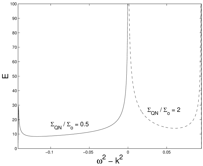
Figure 4: This figure shows the energy E as a function of $\omega^{2}-k^{2}$, in the mangetic regime ($\Sigma_{QN}/\Sigma_{o}=0.5$ on the left), and in the electric regime ($\Sigma_{QN}/\Sigma_{o}=2$ on the right).

The last point is to check the required condition that $\mu^{2}-\frac{\lambda_{\sigma}}{4}\Sigma_{4}>0$ when $\omega^{2}-k^{2}\simeq 0$. But in this case, $\mu$ and $\Sigma_{4}$ tend to their chiral limits, and we have already proved in eq. (26) that in this limit, this quantity is positive, $\mathcal{E}_{k=\omega=0}>0$ . So this in turn ensures that the condition for the existence of a vorton holds for the whole magnetic and electric regime, except in the limiting cases where $\Sigma_{QN}=0$ or $\Sigma_{QN}=\infty$.

Limiting cases $Q=0$ and $N=0$:

Let us first consider the first of these cases, the so-called spring [5, 14], with no charge on the loop. It is possible to study analytically the behaviour of these objects in this model, if one further assumes that there is no backreaction of the condensate on the vortex field. This is a legitimate first approximation, if we consider the profiles shown on fig. 1. Then, with our ansatze (22), we are able to differentiate (28) with respect to $k$ (note that $\Sigma_{QN}=0$), from which we obtain a polynomial in $v=-k^{2}/k_{c}^{2}$:

$$P(v)\equiv\frac{(1-v)^{2}}{N}\frac{d{\mathcal{E}}}{dk} = \frac{\lambda_{\sigma}}{4}\Sigma_{4o}v^{3}-(\mu+\frac{5\lambda_{\sigma}}{4}\Sigma_{4o})v^{2}$$ (29)

$$+(\mu-\frac{5\lambda_{\sigma}}{4}\Sigma_{4o})v-\mu+\frac{\lambda_{\sigma}}{4}\Sigma_{4o}\,.$$

No springs will form if $P$ is always negative. Since we are restricted to the interval $-1<v<0$ and as both $P(0)<0$ and $P(-1)<0$, this will be the case if the derivative $P^{\prime}$ never vanishes between $0$ and $-1$. Now $P^{\prime}$ is a second order polynomial, and some algebra shows that it has a negative minimum for $v>0$. Thus, it is enough to check that $P^{\prime}(0)=2\mu-\frac{5\lambda_{\sigma}}{4}\Sigma_{4o}>0$ (it can be seen that $P^{\prime}(-1)>0$ by direct computation). To prove this, we note that:

$$\frac{\lambda_{\sigma}}{4}\Sigma_{4o}<\frac{\lambda_{\sigma}}{4}\frac{\eta_{\sigma}^{4}}{m_{o}^{2}}\mathrel{\hbox to0.0pt{\lower 4.0pt\hbox{\hskip 1.0pt$\sim$}\hss}\raise 1.0pt\hbox{$<$}}\eta_{\sigma}^{2}<\frac{\eta_{\phi}^{2}}{2}\simeq\frac{\mu}{4\pi}\,,$$ (30)

where we have assumed that $\frac{\lambda_{\sigma}}{2}\frac{\eta_{\sigma}^{2}}{m_{o}^{2}}\mathrel{\hbox to0.0pt{\lower 4.0pt\hbox{\hskip 1.0pt$\sim$}\hss}\raise 1.0pt\hbox{$<$}}2$, and that the string energy density is not too different from its critical coupling value. This indicates that for reasonable parameters, spring formation is excluded. The behaviour of the energy functional is shown in fig. 5. Of course, for the gauged case it is possible that additional terms from magnetic pressure could stabilise the configuration from collapse [5]. However, since these are logarithmic corrections, such gauged springs could only exist on astrophysical scales.

We have also studied the energetic behaviour of the Q-loop, with $N=0$. In this case, we can rewrite the energy functional as:

$$\mathcal{E}_{Q}=(\mu-\frac{\lambda_{\sigma}}{4}\Sigma_{4})\frac{Q}{\omega\Sigma}+2\omega Q\,.$$ (31)

The typical behaviour of this functional as $\omega$ varies is shown on fig. 5. As can be seen, there does not appear to be any stable configuration, since the minimum of the energy is for $\omega=\omega_{c}$, that is for $L=0$.

Figure 5: This figure shows the behaviour of the energy functional for the spring ($E$ is plotted as a function of $k^{2}$) and the Q-loop ($E$ is then a function of $\omega^{2}$). It seems that no stable configuration of finite radius can be expected from these configurations.

5 The stability of the superconducting current

We have seen in the previous section that the model derived from (1) seems to lead to stable loop solutions, but the issue of classical stability has not yet been addressed in a full analytic treatment (for the quantum stability, refer to [15]). This analysis is inspired in part by a heuristic argument in ref. [16] suggesting that classical instabilities could develop in currents with sufficiently high winding. Because of the Lorentz invariance of the theory, we have only 3 cases to consider: pure current ($\omega=0$), pure charge ($k=0$), and the chiral case $\omega=k$. In this section, we wish to study the perturbations around the pure current solution. To proceed, we decompose our field in the following way: $\sigma=S_{k}(r)(e^{ikz}+\nu(z))$, where $S_{k}$ is the radial part of the unperturbed solution and $\nu$ is an arbitrary perturbation.

The change in $\mathcal{E}_{\sigma}$ is easily computed:

$$\delta^{2}\mathcal{E}_{\sigma}=\int dz\left(\Sigma_{2}|\nabla_{z}\nu|^{2}+\gamma|\nu|^{2}+\frac{\lambda_{\sigma}}{4}\Sigma_{4}[e^{-ikz}\nu+e^{ikz}\nu^{+}]^{2}\right)\,,$$ (32)

where

$$\gamma=\int dS\,(|\nabla_{r}S_{k}|^{2}+\frac{\lambda_{\sigma}}{2}S_{k}^{4}+(\beta|\phi|^{2}-\frac{1}{2}\lambda_{\sigma}\eta_{\sigma}^{2})S_{k}^{2})=\mathcal{E}_{\sigma}+\frac{\lambda_{\sigma}}{4}\Sigma_{4}-k^{2}\Sigma\,.$$ (33)

Now to simplify the expression (33) for $\gamma$, we can make use of our analytic result for $\mathcal{E}_{\sigma}$ (15) to find that $\gamma=-k^{2}\Sigma$. We can now rewrite the eigenvalue equation (following the method used in [17]):

$$-\Sigma_{2}\nabla_{z}^{2}\nu+\gamma\nu+\frac{\lambda_{\sigma}}{2}\Sigma_{4}[\nu+\nu^{+}e^{2ikz}]=\lambda\nu\,.$$ (34)

To simplify this equation further, consider expanding our perturbation $\nu$ in the form $\nu=e^{ikz}[u_{1}+iu_{2}]$. Substitution leads to the system of coupled equations:

$$-\Sigma\nabla_{z}^{2}u_{1}+2\Sigma k\nabla_{z}u_{2}+(k^{2}\Sigma+\gamma+\lambda_{\sigma}\Sigma_{4}-\lambda)u_{1}=0\,,$$ (35)

$$-\Sigma\nabla_{z}^{2}u_{2}-2\Sigma k\nabla_{z}u_{1}+(k^{2}\Sigma+\gamma-\lambda)u_{2}=0\,.$$ (36)

To solve this system, we expand in Fourier modes, $u_{i}=a_{i}e^{ipz}$, and we use our simple expression for $\gamma$ to obtain the following set of linear equations:

$$(\Sigma p^{2}+\lambda_{\sigma}\Sigma_{4}-\lambda_{p})a_{1}+2i(k.p)\Sigma a_{2}=0\,,$$ (37)

$$(\Sigma p^{2}-\lambda_{p})a_{2}-2i(k.p)\Sigma a_{1}=0\,.$$ (38)

The vanishing of the determinant of this system yields our eigenvalues:

$$\lambda_{p}=p^{2}\Sigma+\frac{\lambda_{\sigma}}{2}\Sigma_{4}\pm\sqrt{\left(\frac{\lambda_{\sigma}}{2}\Sigma_{4}\right)^{2}+4\Sigma^{2}(k.p)^{2}}\,.$$ (39)

Instabilities will occur when one of the possible $\lambda_{p}$ is negative, which is equivalent to the condition

$$\Sigma^{2}p^{4}+4p^{2}\Sigma(\frac{\lambda_{\sigma}}{4}\Sigma_{4}-k^{2}\Sigma)<0\,,$$ (40)

which leads to:

$$\frac{\lambda_{\sigma}}{4}\Sigma_{4}-k^{2}\Sigma<0$$ (41)

With our ansatz (19) for the moments $\Sigma_{2},\,\Sigma_{4}$, we can use this result to determine the critical value of $k_{\rm inst}$ above which a current becomes unstable:

$$k^{2}_{\rm inst}=\frac{\alpha k_{c}^{2}}{\alpha+k_{c}^{2}}\,,$$ (42)

where $\alpha=\frac{\lambda_{\sigma}}{4}\Sigma_{4o}/\Sigma_{o}$ and $k_{c}^{2}$ is given by (9). Typically, the coefficient $\alpha$ is of order unity, and so we can expect $k_{\rm inst}^{2}\simeq k^{2}_{c}/2$, in good agreement with numerical estimates. We contrast this quantitatively with the heuristic result given in ref. [16] which suggested that the onset of instability was indicated by the condition $\frac{\partial J}{\partial k}<0$; our numerical estimates indicate that the precise criterion (42) is significantly lower.

Note also that through (40), we are able to predict the associated wavenumber $p$ and hence the typical lengthscale of the perturbation for a given unstable current with $k>k_{\rm inst}$. Again, this is in good agreement with our simulations. (Strictly speaking, a more accurate analysis should take into account the effects of charge conservation; we will discuss this more elaborate calculation elsewhere [18], but we note that it yields the same result (42).)

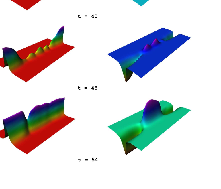
Figure 6: Modulus (left column) and real part (right column) of the condensate along the string axis at various stages of its evolution, showing the current instability. We clearly see that the condensate looses quanta of winding in this process

We point out that this analysis has been carried out by looking only at the condensate part of the energy. Therefore, it is valid in a broader class of models than the one we are considering here, since the vortex is somehow irrelevant. In particular, this instability may appear in any model exhibiting a second-order $U(1)$ phase transition, and could be applied in e.g. superconductivity studies of resistive transition.

Our three-dimensional field theory code allows us to follow the development and evolution of these perturbations and their consequences for the structure of the superconducting string. From fig. 6, we see that the condensate becomes pinched as the instability develops; if the winding number is sufficiently high, the instability will force the condensate down such that $\sigma=0$ at a localised point along the string. This allows the string to lose quanta of winding and lowers $k$ in this region. The condensate then bounces back and slowly relaxes into the stable current configuration, radiating the energy difference between the initial and the final configuration. These numerical results are provided by way of illustration but a more extensive study will be reported shortly with further details about the simulation code [18].

6 Conclusions and prospects

In this paper we have studied the behaviour and effects of the currents and charges on superconducting strings and loops. We have derived exact formulae for the energy of a loop, which exhibits a generic divergence at $\omega^{2}-k^{2}=0$, therefore proving that the chiral case is not an attractor, but rather a repeller.

Since for stable configurations we typically have $\Sigma\simeq\Sigma_{QN}\equiv Q/N$, from (27) we can expect the final size of the loop to be very much smaller than its original size (for realistic initial conditions). Of course, we have not taken into account the vortex-antivortex interactions on scales small compared to the string width, so the inevitability of vorton formation is subject to this important caveat. In addition we conclude that springs and Q-loops are not allowed in this theory.

Studying the stability of the current on a straight string, we have also seen that the superconducting regime is unstable when the winding is too high. By Lorentz-invariance, it is easy to see that this will be the case if $m_{o}^{2}v=k^{2}-\omega^{2}>k_{\rm inst}^{2}$, where $m_{o}^{2}\simeq k^{2}_{c}\simeq\omega_{c}^{2}$. (We believe that the gauged case will exhibit the same generic features as these global currents, though with the small quantitative differences already discussed.)

Now, from our analysis of the vorton state, we know that equilibrium typically will be achieved when $\Sigma\simeq\Sigma_{QN}$. Using our ansatz (22), this is equivalent to

$$v\simeq\frac{\Sigma_{QN}-\Sigma_{o}}{\Sigma_{QN}+\Sigma_{o}}\,.$$ (43)

To ensure stability, we have to impose $v>-k_{\rm inst}^{2}/m_{o}^{2}$ which, with (43) and some algebra, leads to the condition

$$\Sigma_{QN}>\frac{m_{o}^{2}-k_{\rm inst}^{2}}{m_{o}^{2}+k_{\rm inst}^{2}}\,\Sigma_{o}\,.$$ (44)

Loops that do not satisfy (44) will be unstable and lose quanta of winding. Hence, $\Sigma_{QN}$ will increase, and the loop may reach a stable state. This process is associated with energy radiation, which would be interesting to quantify to determine possible observational signatures of this phenomenon.

Finally, the perturbative stability analysis carried out for superconducting currents in the magnetic regime has been extended to the chiral and electric cases, and appears to establish their stability. However, this issue is more subtle, and the analysis will be published separately [18].

References

- [1] A. Vilenkin and E. P. S. Shellard. Cosmic Strings and Other Topological Defects. Cambridge University Press, 2000.
- [2] E. Witten. Superconducting strings. Nucl. Phys., B249:557, 1985.
- [3] R. Davis and E.P.S. Shellard. The physics of vortex superconductivity i: currents and quenching. Phys. Lett., 207B:404, 1988.
- [4] R. Davis and E.P.S. Shellard. The physics of vortex superconductivity ii: charge, angular momentum and the vorton. Phys. Lett., 209B:485, 1988.
- [5] D. Haws, M. Hindmarsch, and N. Turok. Superconducting strings or springs. Phys. Lett., 209B:255, 1988.
- [6] P. Laguna and R. M. Matzner. Numerical simulations of bosonic superconducting strings interactions. Phys. Rev., D41:1751, 1990.
- [7] R. L. Davis and E. P. S. Shellard. Cosmic vortons. Nucl. Phys., B323:209–224, 1989.
- [8] C. J. A. P. Martins and E. P. S. Shellard. Vorton formation. Phys. Rev., D57:7155–7176, 1998.
- [9] B. Carter and A. C. Davis. Chiral vortons and cosmological constraints on particle physics. Phys. Rev., D61, 2000.
- [10] B. Carter and P. Peter. Dynamics and integrability property of the chiral string model. Phys. Lett., B466:41–49, 1999.
- [11] J. J. Blanco-Pillado, K. D. Olumn, and A. Vilenkin. Dynamics of superconducting strings with chiral currents. Phys. Rev., D63, 2001.
- [12] A. C. Davis, T. W. B. Kibble, M. Pickles, and D. A. Steer. Dynamics and properties of chiral cosmic strings in minkowski space. Phys. Rev., D62:083516, 2000.
- [13] M. Pickles and A. C. Davis. Dynamics and properties of chiral cosmic strings. Phys. Lett., B520:345–352, 2001.
- [14] E. J. Copeland, N. Turok, and M. Hindmarsch. Dynamics of superconducting cosmic strings. Phys. Rev. Lett., 58:190, 1987.
- [15] J. J. Blanco-Pillado, K. D. Olum, and A. Vilenkin. Quantum tunneling of superconducting string currents. Phys. Rev., D66:23506, 2002.
- [16] C. Thomson. PhD thesis, Princeton University, 1988.
- [17] J. S. Langer and V. Ambegaokar. Intrisic resistive transition in narrow superconducting channels. Phys. Rev., 164:498–510, 1967.
- [18] Y. F. J. Lemperiere and E. P. S. Shellard. Dynamics of chiral superconducting cosmic strings. DAMTP preprint, 2002.
- [19] J.N. Moore. Gauged Vortices, Dynamics, radiation and cosmological network. PhD thesis, University of Cambridge, 2000.
- [20] J. N. Moore, E. P. S. Shellard, and C. J. A. P. Martins. On the evolution of abelian-higgs string networks. Phys. Rev., D65:023503, 2002.