Condensates in Quantum Chromodynamics

Abstract

The paper presents the short review of our to-day knowledge of vacuum condensates in QCD. The condensates are defined as vacuum averages of the operators which arise due to nonperturbative effects. The important role of condensates in determination of physical properties of hadrons and of their low-energy interactions in QCD is underlined. The special value of quark condensate, connected with the existence of baryon masses is mentioned. Vacuum condensates induced by external fields are discussed. QCD at low energy is checked on the basis of the data on hadronic $\tau$-decay. In the theoretical analysis the terms of perturbation theory (PT) up to $\alpha^{3}_{s}$ are accounted, in the operator product expansion (OPE) - those up to dimension 8. The total probability of the decay $\tau\to hadrons$ (with zero strangeness) and of the $\tau$-decay structure functions are best described at $\alpha_{s}(m^{2}_{\tau})=0.330\pm 0.025$. It is shown that the Borel sum rules for $\tau$-decay structure functions along the rays in the $q^{2}$-complex plane are in agreement with the experiment with the accuracy $\sim 2\%$ at the values of the Borel parameter $|M^{2}|>0.8GeV^{2}$. The magnitudes of dimensions 6 and 8 condensates were found and the limitations on gluonic condensates were obtained. The sum rules for the charmed quark vector currents polarization operator was analysed in 3 loops (i.e., in order $\alpha^{2}_{s}$). The value of charmed quark mass (in $\overline{MS}$ regularization scheme) was found to be: $\overline{m}_{c}(\overline{m}_{c})=1.275\pm 0.015GeV$ and the value of gluonic condensate was estimated: $\langle 0|(\alpha_{s}/\pi)G^{2}|0\rangle=0.009\pm 0.007GeV^{4}$. The general conclusion is: QCD described by PT + OPE is in a good agreement with experiment at $Q^{2}\mathrel{\mathchoice{\lower 3.6pt\vbox{\halign{$\mathsurround=0pt\displaystyle\hfil#\hfil$\cr>\crcr\sim\crcr}}}{\lower 3.6pt\vbox{\halign{$\mathsurround=0pt\textstyle\hfil#\hfil$\cr>\crcr\sim\crcr}}}{\lower 3.6pt\vbox{\halign{$\mathsurround=0pt\scriptstyle\hfil#\hfil$\cr>\crcr\sim\crcr}}}{\lower 3.6pt\vbox{\halign{$\mathsurround=0pt\scriptscriptstyle\hfil#\hfil$\cr>\crcr\sim\crcr}}}}1GeV^{2}$.

1. A few words about Igor’ Vasilyevich.

It is a great honour and at the same time a great pleasure for me to write a paper to the issue of Physics of Atomic Nuclei dedicated to 100-anniversary of Igor’ Vasilyevich Kurchatov birthday. Kurchatov was a very extraordinary person: an organizer of the highest class, I know nobody with such excellent organization abilities. Without him, the soviet atomic project would not be, perhaps, realized, at the least in such short time. Igor’ Vasilyevich had the strongest sense of responsibility not only for the work entrusted to him – the atomic project – but for the much wider – for the fortune of the science in our country and moreover, for the fortune of the whole mankind. I shall give an episod not well known. As witnesses A.P.Aleksandrov [1], Kurchatov was deeply depressed when coming back from the tests of the first hydrogen bomb (those who were present at the tests noticed the same). He said: ”What a terrible thing we have made. The only item we should bother about, is to forbid all of this and to exclude nuclear war”. In March 1954 Kurchatov, Alikhanov, Kikoin and Vinogradov had written the paper, where they concluded, that ”– the mankind is in front of the menace of the end of all of the life on the Earth”. The paper was also signed by the Minister of the Middle Machine Building V.A.Malyshev who had sent it to Malenkov, Khrushchev and Molotov. Khrushchev, however, had rejected the paper, calling the words on a possible ruin of the world civilization ”theoretically wrong and politically harmful” (see [2]). The position of the soviet leaders remained as before: the world war should lead to the ruin of the capitalism.

The same responsibility was inherent to Igor’ Vasilyevich when constructing atomic reactors and atomic powerstations – I gave examples of this earlier [3]. I think that if Kurchatov would alive, RBMK reactors, principally not safe as physical systems, would not be constructed and we would avoid the Chernobyl catastrophe. But on the other hand, Igor’ Vasilyevich was a person of his time … (see [3]).

He liked the science and, in the first turn, his main speciality-nuclear physics. He was deeply interested in the development of the elementary particle physics and he thought that it is necessary to develop such investigations in the USSR. He supported the suggestion of Alikhanov and Vladimirsky of construction at ITEP of the 7 GeV hard-focusing proton accelerator, and then, using the ITEP project, of the 50 GeV proton accelerator (later, 70 GeV) near Serpukhov. In 1954 such decision had been adopted at the meeting of the chaired by Kurchatov Scientific-Technical Council of the Middle Machine-Building Ministry.

2. Introduction

Nowadays, it is reliably established that the true (microscopic) theory of strong interaction is quantum chromodynamics (QCD), the gauge theory of interacting quarks and gluons. It is also established, that unlike, e.g., quantum electrodynamics (QED), the vacuum in QCD has a nontrivial structure: due to nonperturbative effects, i.e. not admitting the expansion in the interaction constant (even if it is small) in QCD vacuum persist non-zero fluctuations of gluonic and quark fields. (Examples of such kind of nonperturbative fields are instantons [4] – classical solutions of equations for gluonic field, which realize the minimum of actions in the QCD Lagrangian. The nontrivial structure in QCD manifests itself in the presence of vacuum condensates, analogous to those in the condensed matter physics (for instance, spontaneous magnetization). Vacuum condensates are very important in elucidation of the QCD structure and in description of hadron properties at low energies. Condensates, in particular, quark and gluonic ones, were investigated starting from 70-ties. Here, first, it should be noted the QCD sum rule method by Shifman, Vainshtein, and Zakharov [5], which was based on the idea of the leading role of condensates in the calculation of masses of the low-lying hadronic states. In the papers of 70-80-ies it was adopted that the perturbaive interaction constant is comparatively small (e.g., $\alpha_{s}(1GeV)\approx 0.3)$, so that it is enough to restrict oneself by the first-order terms in $\alpha_{s}$ and sometimes even disregard perturbative effects in the region of masses larger than 1 GeV. At present it is clear that $\alpha_{s}$ is considerably larger ($\alpha_{s}(1GeV)\sim 0.6$). In a number of cases there appeared the results of perturbative calculations in order $\alpha^{2}_{s}$ and $\alpha^{3}_{s}$. New, more precise experimental data at low energies had been obtained. Thereby, on one hand, it is necessary, and on the other it appears to be possible to compare QCD with the experiment in the low energy region on a higher level of precision. The results of such a comparison are presented in this paper.

In Section 3 I define condensates, describe their properties and give numerical values which were obtained previously. In Section 4, the data on hadronic decays of $\tau$-lepton are compared with theoretical expectations obtained on the basis of the operator product expansion in QCD with the account of perturbative terms up to $\alpha^{3}_{s}$. The values of condensates and the coupling constant $\alpha_{s}(m^{2}_{\tau})$ are obtained. In Section 5, polarization operator of the vector current of charmed quarks is analysed in three-loop approximation (i.e., with the account of the terms $\sim\alpha^{2}_{s}$), the value of the charmed quark and the value of gluonic condensate are found. Section 6 presents our conclusions.

3. Definition of condensates, their main properties

In QCD (or in a more general case, in quantum field theory) by condensates there are called the vacuum mean values $\langle 0|O_{i}|0\rangle$ of the local (i.e. taken at a single point of space-time) of the operators $O_{i}(x)$, which arise due to nonperturbative effects. The latter point is very important and needs clarification. When determining vacuum condensates one implies the averaging only over nonperturbative fluctuations. If for some operator $O_{i}$ the non-zero vacuum mean value appears also in the perturbation theory, it should not be taken into account in determination of the condensate – in other words, when determining condensates the perturbative vacuum mean values should be subtracted in calculation of the vacuum averages. One more specification is necessary. The perturbation theory series in QCD are asymptotic series. So, vacuum mean operator values may appear due to one or another summing of asymptotic series. The vacuum mean values of such kind are commonly to be referred to vacuum condensates.

Separation of perturbative and nonperturbative contributon into vacuum mean values has some arbitrariness. Usually [6,7], this arbitrariness is avoided by introduction of some normalization point $\mu^{2}$   ($\mu^{2}\sim 1GeV^{2}$). Integration over momenta of virtual quarks and gluons in the region below $\mu^{2}$ is referred to condensates, above $\mu^{2}$ – to perturbative theory. In such a formulation condensates depend on the normalization point $\mu$:   $\langle 0|O_{i}|0\rangle=\langle 0|O_{i}|0\rangle_{\mu}$. Other methods for determination of condensates are also possible (see below).

In perturbation theory, there appear corrections to the condensates as a series in the coupling constant $\alpha_{s}(\mu)$:

$$\langle 0|O_{i}|0\rangle_{Q}=\langle 0|O_{i}|0\rangle_{\mu}\sum\limits^{\infty}_{n=0}~{}C^{(i)}_{n}(Q,\mu)\alpha^{n}_{s}(\mu)$$ (1)

The running coupling constant $\alpha_{s}$ at the right-hand part of (1) is normalized at the point $\mu$. The left-hand part of (1) represents the value of the condensate normalized at the point $Q$. Coefficients $C^{(i)}_{n}(Q,\mu)$ may have logarithms $lnQ^{2}/\mu^{2}$ in powers up to $n$ for $C^{(i)}_{n}$. Summing up of the terms with highest powers of logarithms leads to appearance of the so-called anomalous dimension of operators, so that in general form it can be written

$$\langle 0|O_{i}|0\rangle=\langle 0|O_{i}|0\rangle_{\mu}\Biggl{(}\frac{\alpha_{s}(\mu)}{\alpha_{s}(Q)}\Biggr{)}^{\gamma}\sum\limits^{\infty}_{n=0}~{}c^{(i)}_{n}(Q,\mu)\alpha^{n}_{s}(\mu),$$ (2)

where $\gamma$ - is anomalous dimension (number), and $c^{(i)}_{n}$ has already no leading logarithms. If there exist several operators of the given (canonical) dimension, then their mixing is possible in perturbation theory. Then the relations (1),(2) become matrix ones.

In their physical properties condensates in QCD have much in common with condensates appearing in condensed matter physics: such as superfluid liquid (Bose-condensate) in liquid ${}^{4}He$, Cooper pair condensate in superconductor, spontaneous magnetizaion in magnetic etc. That is why, analogously to effects in the physics of condensed matter, it can be expected that if one considers QCD at finite temperature $T$, with $T$ increasing at some $T=T_{c}$ there will be phase transition and condensates (or a part of them) will be destroyed. Particularly, such a phenomenon must hold for condensates responsible for spontaneous symmetry breaking – at $T=T_{c}$ they should vanish and symmetry must be restored. (In principle, surely, QCD may have a few phase transition).

Condensates in QCD are divided into two types: conserving and violating chirality. As is known, the masses of light quarks $u,d,s$ in the QCD Lagrangian are small comparing with the characteristic scale of hadronic masses $M\sim 1GeV$. In neglecting light quark masses the QCD Lagrangian becomes chiral-invariant: left-hand and right-hand (in chirality) light quarks do not interact with each other, both vector and axial currents are conserved (except for flavour-singlet axial current, non-conservation of which is due to anomaly). The accuracy of light quark masses neglect corresponds to the accuracy of isotopical symmetry, i.e. a few per cent in the case of $u$ and $d$ quarks and of the accuracy of SU(3) symmetry, i.e. 10-15 % in the case of $s$-quarks. In the case of condensates violating chiral symmetry, perturbative vacuum mean values are proportional to light quark masses and are zero within $m_{u}=m_{d}=m_{s}=0$. So, such condensates are determined in the theory much better than those conserving chirality and, in principle, may be found experimentally with higher accuracy.

Among chiral symmetry violating condensates of the most importance is the quark condensate $\langle 0|\bar{q}q|0\rangle$  ($q=u,d$ are the fields of $u$ and $d$ quarks). $\langle 0|\bar{q}q|0\rangle$ may be written in the form

$$\langle 0|\bar{q}q|0\rangle=\langle 0|\bar{q}_{L}q_{R}+\bar{q}_{R}q_{L}|0\rangle$$ (3)

where $q_{L},q_{R}$ are the fields of left-hand and right-hand (in chirality) quarks. As follows from (3), the non-zero value of quark condensate means the transition of left-hand quark fields into right-hand ones and its not a small value would mean to chiral symmetry violation in QCD. (If chiral symmetry is not violated, then at small $m_{u},m_{d}$    $\langle 0|\bar{q}q|0\rangle\sim m_{u},m_{d}$). By virtue of isotopical invariance

$$\langle 0|\bar{u}u|0\rangle=\langle 0|\bar{d}d|0\rangle$$ (4)

For quark condensate there holds the Gell-Mann-Oakes-Renner relation [8]

$$\langle 0|\bar{q}q|0\rangle=-\frac{1}{2}~{}\frac{m^{2}_{\pi}f^{2}_{\pi}}{m_{u}+m_{d}}$$ (5)

Here $m_{\pi},f_{\pi}$ are the mass and constant of $\pi^{+}$-meson decay ($m_{\pi}=140MeV,~{}f_{\pi}=131MeV$),   $m_{u}$ and $m_{d}$ are the masses of $u$ and $d$-quarks. Relation (5) is obtained in the first order in $m_{u},m_{d},m_{s}$ (for its derivation see, e.g. [9]). To estimate the value of quark condensate one may use the values of quark masses $m_{u}=4.2MeV$,   $m_{d}=7.5MeV$ [9]. (These values were suggested by Weinberg [10], within the errors they coincide with other estimates – see, for example, [11]). Substituting these values into (5) we get

$$\langle 0|\bar{q}q|0\rangle=-(243MeV)^{3}$$ (6)

The value (6) has characteristic hadronic scale. This shows that chiral symmetry which is fulfilled with a good accuracy in the light quark lagrangian ($m_{u},m_{d}/M\sim 0.01$, $M$ - is hadronic mass scale, $M\sim 0.5-1GeV$), is spontaneously violated on hadronic state spectrum.

An other argument in the favour of spontaneous violation of chiral symmetry in QCD is the existence of massive baryons. Indeed, in the chiral-symmetrical theory all fermionic states should be either massless or parity-degenerated. Obviously, baryons, in particular, nucleon do not possess this property. It can be shown [12, 9], that both these phenomena – the presence of the chiral symmetry violating quark condensate and the existence of massive baryons are closely connected with each other. According to the Goldstone theorem, the spontaneous symmetry violation leads to appearance of massless particles in the physical state spectrum – of Goldstone bosons. In QCD Goldstone bosons can be identified with a $\pi$-meson triplet within $m_{u},m_{d}\to 0$,   $m_{s}\not=0$ (SU(2)-symmetry) or with an octet of pseudoscalar mesons ($\pi$, $K,\eta$) within the limit $m_{u},m_{d},m_{s}\to 0$ (SU(3)-symmetry). The presence of Goldstone bosons in QCD makes it possible to formulate the low-energy chiral effective theory of strong interactions (see reviews [13], [14], [9]).

Quark condensate may be considered as an order parameter in QCD corresponding to spontaneous violation of the chiral symmetry. At the temperature of restoration of the chiral symmetry $T=T_{c}$ it must vanish. The investigation of the temperature dependence of quark condensate in chiral effective theory [15] (see also the review [9]) shows that $\langle 0|\bar{q}q|0\rangle$ vanishes at $T=T_{c}\approx 150-200MeV$. Similar indications were obtained also in the lattice calculations [16].

Thus, the quark condensate: 1)has the lowest dimensions (d=3) as compared with other condensates in QCD; 2) determines masses of usual (nonstrange) baryons; 3) is the order parameter in the phase transition between the phases of violated and restored chiral symmetry. These three facts determine its important role in the low-energy hadronic physics.

Let us estimate the accuracy of numerical value of (6). The Gell-Mann-Oakes-Renner relation is derived up to correction terms linear in quark masses. In the chiral effective theory one succeeds in estimating the correction terms and,thereby, the accuracy of equation (5) appears of order 10%. However, it is not a single origin of errors in determination of quark condensate value. The quark condensate, as well as quark masses depend on the normalization point and have anomalous dimensions equalling to $\gamma_{m}=-\gamma_{\bar{q}q}=\frac{4}{9}$. In the mass values taken above the normalization point $\mu$ was not fixed exactly (in fact, it was taken $\mu\sim 1GeV$). In addition, the accuracy of the above taken value $m_{u}+m_{d}=11.7MeV$ which enters (5) seems to be of order $10-20\%$. The value of the quark condensate may be also found from the sum rules for proton mass. The analysis made [17] gave for it a value very close to (6) (with the 3$\%$ difference) at the normalization point $\mu=1GeV$. The accuracy of these sum rules seems to be of order 10-15$\%$. Concludingly, it may be believed, that the value of the quark condensate is given by (6) at the normalization point $\mu=1GeV$ with the 10-20$\%$ accuracy. The quark condensate of strange quarks is somewhat different from $\langle 0|\bar{u}u|0\rangle$. In [12] it was obtained

$$\langle 0|\bar{s}s|0\rangle/\langle 0|\bar{u}u|0\rangle=0.8\pm 0.1$$ (7)

The next in dimension (d = 5) condensate which violates chiral symmetry is quark gluonic one:

$$-g\langle 0|\bar{q}\sigma_{\mu\nu}\frac{\lambda^{n}}{2}G^{n}_{\mu\nu}q|0\rangle\equiv m^{2}_{0}\langle 0|\bar{q}q|\rangle$$ (8)

Here $G^{n}_{\mu\nu}$ - is the gluonic field strength tensor, $\lambda^{n}$ - are the Gell-Mann matrices, $\sigma_{\mu\nu}=(i/2)(\gamma_{\mu}\gamma_{\nu}-\gamma_{\nu}\gamma_{\mu}$. The value of the parameter $m^{2}_{0}$ was found in [18] from the sum rules for baryonic resonances

$$m^{2}_{0}=0.8GeV^{2}$$ (9)

Consider now condensates conserving chirality. Of fundamental role here is the gluonic condensate of the lowest dimension:

$$\langle 0|\frac{\alpha_{s}}{\pi}G^{n}_{\mu\nu}G^{n}_{\mu\nu}|0\rangle$$ (10)

Due to that the gluonic condensate is proportional to the vacuum mean value of the trace of the energy-momentum tensor $\theta_{\mu\nu}$ its anomalous dimension is zero. The existence of gluonic condensate had been first indicated by Shifman, Vainshtein, and Zakharov [5]. They had also obtained from the sum rules for charmonium its numerical value:

$$\langle 0|\frac{\alpha_{s}}{\pi}G^{n}_{\mu\nu}G^{n}_{\mu\nu}|0\rangle=0.012GeV^{4}$$ (11)

As was shown by the same authors, the nonzero and positive value of gluonic condensate mean, that the vacuum energy is negative in QCD: vacuum energy density in QCD is given by $\varepsilon=-(9/32)\langle 0|(\alpha_{s}/\pi)G^{2}|0\rangle$. Therefore, if quark is embedded into vacuum, this results in its excitation, i.e, in increasing of energy. In this way, the explanation of the bag model could be obtained in QCD: in the domain around quark there appears an excess of energy, which is treated as the energy density $B$ in the bag model. (Although, the magnitude of $B$, does not,probably, agree with the value of $\varepsilon$ which follows from (11)). In ref.[5] perturbative effects were taken into account only in the order $\alpha_{s}$, the value for $\alpha_{s}$ being taken twice as smaller as the modern one. Later many attempts were made to determine the value of gluonic condensate by studying various processes and by applying various methods. But the results of different approaches were inconsistent with each other and with (11) and sometimes the difference was even very large – the values of condensate appeared to be by a few times larger. All of this needs reanalysation of $\langle 0|\frac{\alpha_{s}}{\pi}G^{2}|0\rangle$ determination basing on contemporary values which will be done in Sections 4,5.

The d=6 gluonic condensate is of the form

$$g^{3}f^{abc}\langle 0|G^{a}_{\mu\nu}G^{b}_{\nu\lambda}G^{c}_{\lambda\mu}|0\rangle,$$ (12)

$(f^{abc}$ - are structure constants of SU(3) group). There are no reliable methods to determine it from experimental data. There is only an estimate which follows from the method of deluted instanton gas [19]:

$$g^{3}f^{abc}\langle 0|G^{a}_{\mu\nu}G^{b}{\nu\lambda}G^{c}_{\lambda\mu}|0\rangle=\frac{4}{5}(12\pi^{2})\frac{1}{\rho^{2}_{c}}\langle 0|\frac{\alpha_{s}}{\pi}G^{2}_{\mu\nu}|0\rangle,$$ (13)

where $\rho_{c}$ is the instanton effective radius in the given model (for estimaion one may take $\rho_{c}\sim(1/3-1/2)fm)$.

The general form of d=6 condensates is as follows:

$$\alpha_{s}\langle 0|\bar{q}_{i}O_{\alpha}q_{i}\cdot\bar{q}_{k}O_{\alpha}q_{k}|0\rangle$$ (14)

where $q_{i},q_{k}$ are quark fields of $u,d,s$ quarks, $O_{\alpha}$ - are Dirac and $SU(3)$ matrices. Following [5], Eq.(14) is usually factorized: in the sum over intermediate state in all channels (i.e, if necessary, after Fierz-transformation) only vacuum state is taken into account. The accuracy of such approximation $\sim 1/N^{2}_{c}$, where $N_{c}$ is the number of colours i.e.$\sim 10\%$. After factorizaion Eq.(14) reduces to

$$\alpha_{s}\langle 0|\bar{q}q|0\rangle^{2}$$ (15)

The anomalous dimension of (15) is 1/9 and it can be approximately put to be zero. And finally, d=8 quark condensates assuming factorization reduce to

$$\alpha_{s}\langle 0|\bar{q}q|0\rangle\cdot m^{2}_{0}\langle 0|\bar{q}q|0\rangle$$ (16)

(The notaion of (8) is used). It should be noted, however, that the factorization procedure in the d=8 condensate case is uncertain. For this reason, it is necessary to require their contribution to be small.

Let us also dwell on one more type of condensates - those, induced by external fields. The meaning of such condensates can be easily understood by comparing with analogous phenomena in the physics of condenced media. If the above considered condensates can be compared, for instance with ferromagnetics, where magnetization is present even in the absence of external magnetic field, condensates induced by external field are similar to dia- or paramagnetics. Consider the case of the constant external electromagnetic field $F_{\mu\nu}$. In its presence there appears a condensate induced by external field (in the linear approximation in $F_{\mu\nu}$):

$$\langle 0|\bar{q}\sigma_{\mu\nu}q|0\rangle_{F}=e_{q}\chi F_{\mu\nu}\langle 0|\bar{q}q|0\rangle$$ (17)

As was shown in ref.[20], in a good approximation $\langle 0|\bar{q}\sigma_{\mu\nu}q|0\rangle_{F}$ is proportional to $e_{q}$ - the charge of quark $q$. Induced, by the field vacuum expectation value $\langle 0|\bar{q}\sigma_{\mu\nu}q|0\rangle_{F}$ violates chiral symmetry. So, it is natural to separate $\langle 0|\bar{q}q|0\rangle$ as a factor in Eq.(17). The universal quark flavour independent quantity $\chi$ is called magnetic susceptibility of quark condensate. Its numerical value had been found in [21] using a special sum rule:

$$\chi=-(5.7\pm 0.6)GeV^{2}$$ (18)

Another example is external constant axial isovector field $A_{\mu}$ the interaction of which with light quarks is described by Lagrangian

$$L^{\prime}=(\bar{u}\gamma_{\mu}\gamma_{5}u-\bar{d}\gamma_{\mu}\gamma_{5}d)A_{\mu}$$ (19)

In the presence of this field there appear induced by it condensates:

$$\langle 0|\bar{u}\gamma_{\mu}\gamma_{5}u|0\rangle_{A}=-\langle 0|\bar{d}\gamma_{\mu}\gamma_{5}|0\rangle_{A}=f^{2}_{\pi}A_{\mu}$$ (20)

where $f_{\pi}=131MeV$ is the constant of $\pi\to\mu\nu$ decay. The right-hand part of eq.(20) is obtained assuming $m_{u},m_{d}\to 0,$  $m^{2}_{\pi}\to 0$ and follows directly from consideration of the polarization operator of axial currents $\Pi^{A}_{\mu\nu}(q)$ in the limit $q\to 0$, when nonzero contribution into $\Pi^{A}_{\mu\nu}(q)_{q\to 0}$ emerges only from one-pion intermediate state. The equality (20) was used to calculate the axial coupling constant in $\beta$-decay $q_{A}$ [22]. An analogous to (20) relation holds in the case of octet axial field. Of special interest is the condensate induced by singlet (by flavours) constant axial field

$$\langle 0|\gamma^{(0)}_{\mu 5}|0\rangle=3f^{2}_{0}A^{(0)}_{\mu}$$ (21)

$$j^{(0)}_{\mu 5}=\bar{u}\gamma_{\mu}\gamma_{5}u+\bar{d}\gamma_{\mu}\gamma_{5}d+\bar{s}\gamma_{\mu}\gamma_{5}s$$ (22)

and Lagrangian of interaction with external field has the form

$$L^{\prime}=j^{(0)}_{\mu 5}A^{(0)}_{\mu}$$ (23)

Constant $f_{0}$ cannot be calculated by the method used when deriving eq.(20), since singlet axial current is not conserved by virtue of anomaly and the singlet pseudoscalar meson $\eta^{\prime}$ is not Goldstone one. Constant $f^{2}_{0}$ is proportional to topologicaal susceptibility of vacuum [23]

$$f^{2}_{0}=\frac{4}{3}N^{2}_{f}\chi^{\prime}(0),$$ (24)

where $N_{f}$ is the number of light quarks, $N_{f}=3$, and the topological susceptibility of the vacuum $\chi(q^{2})$ is defined as

$$\chi(q^{2})=i\int~{}d^{4}xe^{iqx}\langle 0|T{Q_{5}(x),~{}Q_{5}(0)}|0\rangle$$ (25)

$$Q_{5}(x)=\frac{\alpha_{s}}{8\pi}G^{n}_{\mu\nu}(x)G^{n}_{\mu\nu}(x)$$ (26)

Using the QCD sum rule, one may relate $f^{2}_{0}$ with the part of proton spin $\Sigma$, carried by quarks in polarized $ep$ (or $\mu p$) scattering [23]. The value of $f^{2}_{0}$ was found from the selfconsistency condition of obtained sum rule (or from the experimental value of $\Sigma$):

$$f^{2}_{0}=(2.8\pm 0.7)\cdot 10^{-2}GeV^{2}$$ (27)

The related to it value of the derivative at $q^{2}=0$ of vacuum topological susceptibility $\chi^{\prime}(0)$, (more precisely, its nonperturbative part) is equal to:

$$\chi^{\prime}(0)=(2.3\pm 0.6)\cdot 10^{-3}GeV^{2}$$ (28)

The value $\chi^{\prime}(0)$ is of essential interest for studying properties of vacuum in QCD.

4. Test of QCD at low energies on the basis of $\tau$-decay data.

Determination of $\alpha_{s}(m^{2}_{\tau})$ and of condensate values.

Recently, collaborations ALEPH [24], OPAL [25] and CLEO [26] had measured with a good accuracy the relative probability of hadronic decays of $\tau$-lepton $R_{\tau}=B(\tau\to\nu_{\tau}+hadrons)/B(\tau\to\nu_{\tau}e\overline{\nu}_{e})$, the vector $V$ and axial $A$ spectral functions. Below I present the results of the theoretical analysis of these data basing on the operator product expansion (OPE) in QCD [27, 28]. In the perturbation theory series the terms up to $\alpha^{3}_{s}$ will be taken into account, in OPE – the operators up to dimension 8.

Consider the polarization operator of hadronic currents

$$\Pi^{J}_{\mu\nu}=i~{}\int~{}e^{iqx}\langle TJ_{\mu}(x)J_{\nu}(0)^{{\dagger}}\rangle dx=(q_{\mu}q_{\nu}-q_{\mu\nu}q^{2})\Pi^{(1)}_{J}(q^{2})+q_{\mu}q_{\nu}\Pi^{(0)}_{J}(q^{2}),$$ (29)

$$\mbox{where}~{}~{}~{}~{}J=V,A;~{}~{}~{}V_{\mu}=\bar{u}\gamma_{\mu}d,~{}~{}~{}A_{\mu}=\bar{u}\gamma_{\mu}\gamma_{5}d.$$

The spectral functions measured in $\tau$-decay are imaginary parts of $\Pi^{(1)}_{J}(s)$ and $\Pi^{(0)}_{J}(s)$,   $s=q^{2}$

$$v_{1}/a_{1}(s)=2\pi Im\Pi^{(1)}_{V/A}(s+i0),~{}~{}~{}a_{0}(s)=2\pi Im\Pi^{(0)}_{A}(s+i0)$$ (30)

Functions $\Pi^{(1)}_{V}(q^{2})$ and $\Pi^{(0)}_{A}(q^{2})$ are analytical functions in the $q^{2}$ complex plane with a cut along the right-hand semiaxis starting from $4m^{2}_{\pi}$ for $\Pi^{(1)}_{V}(q^{2})$ and $9m^{2}_{\pi}$ for $\Pi^{(0)}_{A}(q^{2})$. Function $\Pi^{(1)}_{A}(q^{2})$ has kinematical pole at $q^{2}=0$. This is a specific feature of QCD following from chiral symmetry within massless $u$ and $d$ quarks and from its spontaneous violation. The kinematical pole appears due to one-pion state contribution into $\Pi_{A}(q)$, which has the form [27]

$$\Pi^{A}_{\mu\nu}(q)_{\pi}=-\frac{f^{2}_{\pi}}{q^{2}}(q_{\mu}q_{\nu}-q_{\mu\nu}q^{2})-\frac{m^{2}_{\pi}}{q^{2}}q_{\mu}q_{\nu}\frac{f^{2}_{\pi}}{q^{2}-m^{2}_{\pi}}$$ (31)

Consider first the ratio of the total probability of hadronic decays of $\tau$-lepons into states with zero strangeness to the probability of $\tau\to\nu_{\tau}e\overline{\nu}_{e}$. This ratio is given by the equality [29]

$$R_{\tau,V+A}=\frac{B(\tau\to\nu_{\tau}+hadrons_{S=0})}{B(\tau\to\nu_{\tau}e\bar{\nu}_{e})}=$$

$$=6|V_{ud}|^{2}S_{EW}~{}\int\limits^{m^{2}_{\tau}}_{0}~{}\frac{ds}{m^{2}_{\tau}}\Biggl{(}1-\frac{s}{m^{2}_{\tau}}\Biggr{)}^{2}\Biggl{[}\Biggl{(}1+2\frac{s}{m^{2}_{\tau}}\Biggr{)}(v_{1}+a_{1}+a_{0})(s)-2\frac{s}{m^{2}_{\tau}}a_{0}(s)\Biggr{]}$$ (32)

where $|V_{ud}|=0.9735\pm 0.0008$ is the matrix element of the Kabayashi-Maskawa matrix, $S_{EW}=1.0194\pm 0.0040$ is the electroweak correction [30]. Only one-pion state is practically contributing to the last term in (32) and it appears to be small:

$$\Delta R^{(0)}_{\tau}=-24\pi^{2}\frac{f^{2}_{\pi}m^{2}_{\pi}}{m^{4}_{\tau}}=-0.008$$ (33)

Denote

$$\omega(s)\equiv v_{1}+a_{1}+a_{6}=Im[\Pi^{(1)}_{V}(s)+\Pi{(1)}_{A}(s)+\Pi^{(0)}_{A}(s)]\equiv 2\pi Im\Pi(s)$$ (34)

As follows from eq.(31), $\Pi(s)$ has no kinematical pole, but only right-hand cut. It is convenient to transform the integral in eq.(32) into that over the circle of radius $m^{2}_{\tau}$ in the complex $s$ plane [31]-[33]:

$$R_{\tau,\,V+A}=6\pi i|V_{ud}|^{2}S_{EW}\oint_{|s|=m_{\tau}^{2}}\!{ds\over m_{\tau}^{2}}\left(1-{s\over m_{\tau}^{2}}\right)^{2}\left(1+2{s\over m_{\tau}^{2}}\right)\Pi(s)+\Delta R_{\tau}^{(0)}$$ (35)

Calculate first the perturbative contribution into eq.(35). To this end, use the Adler function $D(Q^{2})$:

$$D(Q^{2})\,\equiv\,-2\pi^{2}\,{d\Pi(Q^{2})\over d\ln{Q^{2}}}\,=\,\sum_{n\geq 0}K_{n}a^{n}\;,\qquad a\equiv{\alpha_{s}\over\pi}\;,\qquad Q^{2}\equiv-s,$$ (36)

the perturbative expansion of which is known up to terms $\sim\alpha^{3}_{s}$. In $\overline{MS}$ regularization scheme $K_{0}=K_{1}=1$,   $K_{2}=1.64$ [34], $K_{3}=6.37$ [35] for 3 flavours and for $K_{4}$ there is the estimate $K_{4}=25\pm 25$ [36]. The renormgroup equation yields

$${da\over d\ln{Q^{2}}}\,=\,-\beta(a)\,=\,-\sum_{n\geq 0}\beta_{n}a^{n+2}\qquad\Rightarrow\qquad\ln{Q^{2}\over\mu^{2}}\,=\,-\,\int_{a(\mu^{2})}^{a(Q^{2})}{da\over\beta(a)},$$ (37)

in the $\overline{MS}$ scheme for three flavours $\beta_{0}=9/4$, $\beta_{1}=4$,   $\beta_{2}=10.06$,   $\beta_{3}=47.23$   [37, 38]. Integrating over eq.(36) and using eq.(38) we get

$$\Pi(Q^{2})\,=\,{1\over 2\pi^{2}}\int_{a(\mu^{2})}^{a(Q^{2})}D(a){da\over\beta(a)}$$ (38)

Put $\mu^{2}=m^{2}_{\tau}$ and choose some (arbitrary) value $a(m^{2}_{\tau})$. With the help of eq.(37) one may determine then $a(Q^{2})$ for any $Q^{2}$ and by analytical continuation for any $s$ in the complex plane. Then, calculating (38) find $\Pi(s)$ in the whole complex plane. Substitution of $\Pi(s)$ into eq.(35) determines $R_{\tau}$ for the given $a(m^{2}_{\tau})$ up to power corrections. Thereby, knowing $R_{\tau}$ from experiment it is possible to find the corresponding to it $a(m^{2}_{\tau})$. Note, that with such an approach there is no need to expand the nominator in eqs.(37), (38) in the inverse powers of $lnQ^{2}/\mu^{2}$. Particularly, there is no expansion on the right-hand semiaxis in powers of the parameter $\pi/ln(Q^{2}/\mu^{2})$, which is not small in the investigated region of $Q^{2}$. Advantages of transformation of the integral over the real axis (32) in the contour integral are the following. It can be expected that the applicability region of the theory presented as perturbation theory (PT) + operator expansion (OPE) in the complex $s$-plane is off the shadowed region in Fig.1. It is evident that at positive and comparatively small $s$ PT+OPE do not work. At negative $s=-Q^{2}$ in $\alpha_{s}$ order a nonphysical pole appears, in higher orders, according with (9) it is replaced by a nonphysical cut, which starts from the point $-Q^{2}_{0}$, determined by the formula

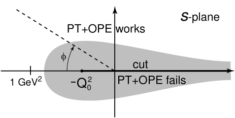
Figure 1: The applicability region of PT and OE in the complex plane $s$. In the dashed region PT + OE does not work.

$$\ln{Q_{0}^{2}\over\mu^{2}}\,=\,-\,\int_{a(\mu^{2})}^{\infty}{da\over\beta(a)}$$ (39)

Integration over the contour allows one to obviate the dashed region in Fig.1 (except for the vicinity of the positive semiaxis, the contribution of which, is suppressed by the factor $(1-\frac{s}{m^{2}_{\tau}})^{2}$ in eq.(6)), i.e. to work in the applicability region of PT+OPE. The OPE terms, i.e., power corrections to polarization operator, are given by the formula (5):

$$\Pi(s)_{nonpert}=\sum_{n\geq 2}{\left<O_{2n}\right>\over(-s)^{n}}\left(1+c_{n}{\alpha_{s}\over\pi}\right){\alpha_{s}\over 6\pi\,Q^{4}}\left<G_{\mu\nu}^{a}G_{\mu\nu}^{a}\right>\left(1+{7\over 6}{\alpha_{s}\over\pi}\right)+$$

$$+{128\over 81\,Q^{6}}\,\pi\alpha_{s}\left<\bar{q}q\right>^{2}\left[1+\left({29\over 24}+{17\over 18}\ln{Q^{2}\over\mu^{2}}\right){\alpha_{s}\over\pi}\right]+{\left<O_{8}\right>\over Q^{8}}$$ (40)

($\alpha_{s}$-corrections to the 1-st and 2-d terms in eq.(39) were calculated in [39] and [40], respectively). Contributions of the operator with $d=2$ proportional to $m^{2}_{u}$, $m^{2}_{d}$ and of the condensate $2(m_{u}+m_{d})\langle 0|\bar{q}q|0\rangle$ are neglected. (The latter is of an order of magnitude smaller than the gluonic condensate contribution). When calculating the d=6 term, factorization hypothesis was used. It can be readily seen that d=4 condensates (up to small $\alpha_{s}$ corrections) give no contribution into the integral over contour eq.(35). The contribution from the condensate $\langle O_{8}\rangle$ may be estimated as $|\langle O_{8}\rangle|<10^{-3}GeV^{8}$ and appears to be negligibly small. $R_{\tau,V+A}$ may be represented as

$$R_{\tau,V+A}=3|V_{ud}|^{2}S_{EW}\left(\,1\,+\,\delta_{EW}^{\prime}\,+\,\delta^{(0)}\,+\,\delta^{(6)}_{V+A}\,\right)+\Delta R^{(0)}~{}=$$

$$=~{}3.475\pm 0.022$$ (41)

where $\delta^{\prime}_{em}=(5/12\pi)\alpha_{em}(m^{2}_{\tau})=0.001$ is electromagnetic correction [41], $\delta^{(6)}_{A+V}=-(5\pm 2)\cdot 10^{-3}$ is the contribution of d=6 condensate (see below) and $\delta^{(0)}$ is the PT correction. The right-hand part presents the experimental value obtained as a difference between the total probability of hadronic decays $R_{\tau}=3.636\pm 0.021$ [42] and the probability of decays in states with the strangeness $S=-1~{}~{}R_{\tau,s}=0.161\pm 0.007$ [43, 44]. For perturbative correction it follows from eq.(41)

$$\delta^{(0)}=0.206\pm 0.010$$ (42)

Employing the above described method in ref.[28] the constant $\alpha_{s}(m^{2}_{\tau})$ was found from (42)

$$\alpha_{s}(m^{2}_{\tau})=0.355\pm 0.025$$ (43)

The calculation was made with the account of terms $\sim\alpha^{3}_{\tau}$, the estimate of the effect of the terms $\sim\alpha^{4}_{s}$ is accounted for in the error. May be, the error is underestimated (by 0.010-0.015), since the theoretical and experimental errors were added in quadratures.

I determine now the values of condensates basing on the data [24] -[26] on spectral functions. It is convenient first to consider the difference $\Pi_{V}-\Pi_{A}$, which is not contributed by perturbative terms and there remains only the OPE contribution:

$$\Pi_{V}^{(1)}(s)-\Pi_{A}^{(1)}(s)\,=\,\sum_{D\geq 4}\,{O^{V-A}_{D}\over(-s)^{D/2}}\left(\,1\,+\,c_{D}{\alpha_{s}\over\pi}\,\right)\,$$ (44)

The gluonic condensates contribution falls out in the $V-A$ difference and only the following condensates with d=4,6,8 remain

$$O^{V-A}_{4}=2\,(m_{u}+m_{d})\,<\bar{q}q>\;=\;-\,f_{\pi}^{2}m_{\pi}^{2}$$ (45)

$$O^{V-A}_{6}=2\pi\alpha_{s}\left<\,(\bar{u}\gamma_{\mu}\lambda^{a}d)(\bar{d}\gamma_{\mu}\lambda^{a}u)-(\bar{u}\gamma_{5}\gamma_{\mu}\lambda^{a}d)(\bar{d}\gamma_{5}\gamma_{\mu}\lambda^{a}u)\,\right>=$$

$$=-\,{64\pi\alpha_{s}\over 9}<\bar{q}q>^{2}$$ (46)

$$O^{V-A}_{8}=8\pi\alpha_{s}\,m_{0}^{2}<\bar{q}q>^{2}\;,$$ (47)

where $m^{2}_{0}$ is determined in eq.(9). In the right-hand of (46),(47) the factorization hypothesis was used. Calculation of the coefficients at $\alpha_{s}$ in eq.(44) gave $c_{4}=4/3$ [39] and $c_{6}=89/48$ [40]. The value of $\alpha_{s}(m^{2}_{\tau})$ (43) corresponds to $\alpha_{s}(1GeV^{2})=0.60$. Thus, if we take for quark condensate at the normlization point $\mu^{2}=1GeV^{2}$ the value (6), then vacuum condensates with the account of $\alpha_{s}$-corrections appear to be equal (at $\mu^{2}=1GeV^{2}$):

$$O_{4}=-4.22\cdot 10^{-4}~{}GeV^{4}$$ (48)

$$O_{6}=-3.75\cdot 10^{-3}~{}GeV^{6}$$ (49)

$$O_{8}=2.5\cdot 10^{-3}~{}GeV^{8}$$ (50)

(In what follows, indeces $V-A$ will be omitted and $O_{D}$ will mean condensates with the account of $\alpha_{s}$ corrections).

Our aim is to compare OPE theoretical predictions with experimental data on $V-A$ structure functions measured in $\tau$-decay and the values of $O_{6}$ and $O_{8}$ found from experiment to compare with eqs.(49),(50). Numerical values of $O_{6}$ and $O_{8}$ (49),(50) do not strongly differ. This indicates that OPE asymptotic series (44) at $Q^{2}=-s\sim 1GeV^{2}$ converge badly and, may be, even diverge and the role of higher dimension operators may be essential. Therefore it is necessary: either to work at larger $Q^{2}$, where, however, experimental errors increase, or to improve the series convergence. The most plausible method is to use Borel transformation. Write for $\Pi^{(1)}_{V}-\Pi^{(1)}_{A}$ the subtractionless dispersion relation

$$\Pi^{(1)}_{V}(s)-\Pi^{(1)}_{A}(s)\,=\,{1\over 2\pi^{2}}\int_{0}^{\infty}{v_{1}(t)-a_{1}(t)\over t-s}\,dt\,+\,{f_{\pi}^{2}\over s}$$ (51)

(The last term in the right-hand part is the kinematic pole contribution). Put $s=s_{0}^{i\phi}$ ($\phi=0$ on the upper edge of the cut) and make the Borel transformation in $s_{0}$. As a result, we get the following sum rules for the real and imaginary parts of (51):

$$\int_{0}^{\infty}\exp{\!\left({s\over M^{2}}\cos{\phi}\right)}\cos{\!\left({s\over M^{2}}\sin{\phi}\right)}(v_{1}-a_{1})(s)\,{ds\over 2\pi^{2}}\,=\,f_{\pi}^{2}+\,\sum_{k=1}^{\infty}(-)^{k}{\cos{(k\phi)}\,O_{2k+2}\over k!\,M^{2k}}$$ (52)

$$\int_{0}^{\infty}\exp{\!\left({s\over M^{2}}\cos{\phi}\right)}\,\sin{\!\left({s\over M^{2}}\sin{\phi}\right)}(v_{1}-a_{1})(s)\,{ds\over 2\pi^{2}M^{2}}\,=\,\sum_{k=1}^{\infty}(-)^{k}{\sin{(k\phi)}\,O_{2k+2}\over k!\,M^{2k+2}}$$ (53)

The use of the Borel transformation along the rays in the complex plane has a number of advantages. The exponent index is negative at $\pi/2<\phi<3\pi/2$. Choose $\phi$ in the region $\pi/2<\phi<\pi$. In this region, on one hand, the shadowed area in fig.1 in the integrals (52),(53) is touched to a less degree, and on the other hand, the contribution of large $s$, particularly, $s>m^{2}_{\tau}$ , where experimental data are absent, is exponentially suppressed. At definite values of $\phi$ the contribution of some condensates vanishes, what may be also used. In particular, the condensate $O_{8}$ does not contribute to (52) at $\phi=5\pi/6$ and to (53) at $\phi=2\pi/3$, while the contribution of $O_{6}$ vanishes at $\phi=3\pi/4$. Finally, a well known advantage of the Borel sum rules is factorial suppression of higher dimension terms of OPE. Figs.2,3 presents the results of the calculations of left-hand parts of eqs.(52),(53) on the basis of the ALEPH [24] experimental data comparing with OPE predictions – the right-hand part of these equations.

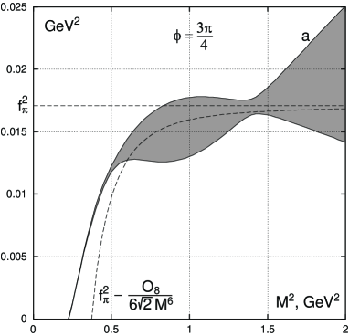
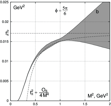
Figure 2: Eq.(52): the left-hand part is obtained basing on the experimental data, the shaded region corresponds to experimental errors; the right-hand part – the theoretical one – is represented by the dotted curve, numerical values of condensates are taken to be equal to the central values of eqs.(54),(55); a) $\phi=3\pi/4$,  b) $\phi=5\pi/6$.

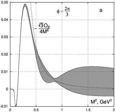
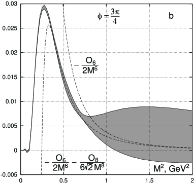
Figure 3: The same for eq.(53): a) $\phi=2\pi/3$,   b) $\phi=3\pi/4$.

The experimental data are best described at the values [27]

$$O_{6}=-(6.8\pm 2.1)\cdot 10^{-3}~{}GeV^{6}$$ (54)

$$O_{8}=-(7\pm 4)\cdot 10^{-3}~{}GeV^{8}$$ (55)

When estimating errors in (54),(55), an uncertainty of higher dimension operator contribution was taken into account in addition to experimental errors. (For detils – see [27]).

As is seen from the figures, at these values of condensates a good agreemeent with experiment starts rather early – at $M^{2}>0.5GeV^{2}$. In paper [27] the sum rules for the moments and the Gaussian sum rules were also considered. All of them agree with the values of condensates (54), (55), but the accuracy of their determination is worse. The values (54),(55) are by a factor of 1.5-2 larger than (49),(50). As was discussed above, the accuracy of (49),(50) is of order 50$\%$. Therefore, the most plausible is that the real value of condensates $O_{6},O_{8}$ is somewhere close to the lower edge of errors in (54),(55).

Consider now the polarization operator $\Pi(s)$ defined in (34) and condensates entering OPE for $\Pi(s)$ (see (40)). In principle, the perturbative terms contribute to chirality conserving condensates. If we will follow the separation method of perturbative and nonperturbative contribution by introducing infrared cut-off [6, 7], then such a contribution would really appear due to the region of virtualities smaller than $\mu^{2}$. In the present paper, according to [28], an another method is exploited, when the $\beta$-function is expanded only in the number of loops, (see eq.(11) and the text after it) but not in $1/lnQ^{2}$. So, the dependence of condensates on the normalization point $\mu^{2}$ is determined only by perturbative corrections, as is seen in (40). Condensates determined in such a way may be called $n$-loop ones (in the given case – 3-loop). Consider the Borel transformation of the sum $\Pi(s)_{pert}+\Pi(s)_{nonpert}$ where $\Pi(s)_{pert}$ is given by eq.(38), and $\Pi(s)_{nonpert}$ – by eq.(13). Fig.4 presents the results of 3-loop calculation for two values of $\alpha_{s}(m^{2}_{\tau})$ – 0.355 and 0.330. The widths of the bands correspond to theoretical error taken to be equal to the last accounted term $K_{3}a^{2}$ in the Adler function (36). (The same result for the error is obtained if one takes 4 loops in $\beta$-function and puts $K_{4}=50\pm 50$). The dotted line corresponds to the sum of contributions of gluonic condensate (11) and $O^{V+A}_{6}$ condensate in (13) with numerical value corresponding to $O^{V-A}_{6}$ (54). The dots with errors present experimental data. (The contribution of the operators $d=4$ and $d=6$ is given separately in the insert).

It is seen that the curve with $\alpha_{s}(m^{2}_{\tau})=0.330$ and condensate contributions can be agreed with experiment, starting from $M^{2}=1.1GeV^{2}$, the agreement being improved at smaller values $\langle 0|\frac{\alpha_{s}}{\pi}G^{2}|0\rangle$ than (11). The curve with $\alpha_{s}(m^{2}_{\tau})=0.355$ with the account of condensates coincides with experiment only at $M^{2}>1.5GeV^{2}$. The same tendency persist for the Borel sum rules taken along the rays in the $s$ complex plane at various $\phi$. Fig.5 gives the sum rule for $\phi=5\pi/6$. From consideration of this and of other sum rules there follows the estimation for gluonic condensate:

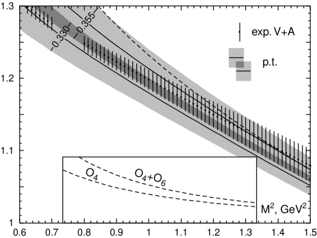
Figure 4: The results of the Borel transformation of $V+A$ correlator for two values $\alpha_{s}(m^{2}_{\tau}=0.355$ and $\alpha_{s}(m^{2}_{\tau})=0.330$. The widths of the bands correspond to PT errors, dots with errors – experimental data. The dotted curve is the sum of the perturbative contribution at $\alpha_{s}(m^{2}_{\tau})=0.330$ and $O_{4}$,  $O_{6}$ condensates.

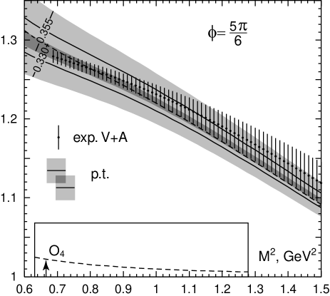
Figure 5: The result of the Borel transformation along the ray at $\phi=5\pi/6$. The dotted line corresponds to the central value of gluonic condensate (56), added to the PT curve with $\alpha_{s}(m^{2}_{\tau})=0.330$.

$$\langle 0\mid\frac{\alpha_{s}}{\pi}G^{a}_{\mu\nu}G^{a}_{\mu\nu}\mid 0\rangle=0.006\pm 0.012~{}GeV^{4}$$ (56)

The best agreement of the theory with experiment in the low $Q^{2}$ region (up to $\sim 2\%$ at $M^{2}>0.8GeV^{2}$) is obtained at $\alpha_{s}(m^{2}_{\tau})=0.330$ which corresponds to $\alpha_{s}(m^{2}_{z})=0.118$.

Let us now make some remarks on modifications of QCD in the low energy region.

1. Analytical perturbative QCD [45], [46]. It is assumed that $\alpha_{s}(q^{2})$ is an analytical function of $q^{2}$ [45], or, in a more general case, it is supposed, that the perturbative part of the polarization operator is an analytical function of $q^{2}$. The comparison of this approach with the $\tau$-decay data showed [28] that in the analytical QCD

$$\alpha^{anal}_{s}(m^{2}_{z})=0.140$$ (57)

what is in a strong disagreement with the world mean value $\alpha_{s}(m^{2}_{z})=0.119\pm 0.002$.

2. Renormalon summing leading to the tachion mass $\lambda^{2}$ in gluon propagator [47]. The restriction to the tachion mass

$$-\lambda^{2}=0.1\pm 0.15~{}GeV^{2}$$ (58)

was found from $\tau$-decay.

3. Instantons. It was shown [28], that in the dilute instanton gas appoximation [48] instantons do not practically affect determination of $\alpha_{s}(m^{2}_{\tau})$ and the Borel sum rules. Their effect, however, appears to be considerable and strongly dependent on the value of the instanton radius $\rho_{c}$ in the sum rules obtained by integration over closed contours in the complex plane $s$ at the radii of the contours $s<2GeV^{2}$.

5. Sum rules for charmonium and gluonic condensate.

The value of gluonic condensate had been found by Shifman, Vainstein, and Zakharov from the sum rules for polarized operator of vector currents of charmed quarks [5]. But in these calculations , the constant $\alpha_{s}$ was taken comparatively small ($\alpha_{s}(1GeV^{2}\approx 0.3$;  $\Lambda^{(3)}_{QCD}=100MeV$) and perturbative corrections were taken into account only in the first order. It is clear now, that $\alpha_{s}(Q^{2})$ in the region $Q^{2}\sim 1\div 10GeV^{2}$ is approximately twice as large, so that the account of higher order corrections became necessary. (In what follows I formulate the main results of [49]).

Consider the polarization operator of charmed vector currents

$$i\int dx\,e^{iqx}\left<\,TJ_{\mu}(x)J_{\nu}(0)\,\right>\,=\,(\,q_{\mu}q_{\nu}-g_{\mu\nu}q^{2}\,)\,\Pi(q^{2})\;,\qquad J_{\mu}=\bar{c}\gamma_{\mu}c$$ (59)

The dispersion representation for $\Pi(q^{2})$ has the form

$$R(s)\,=\,4\pi\,{\rm Im}\,\Pi(s+i0)\;,\qquad\Pi(q^{2})\,=\,{q^{2}\over 4\pi^{2}}\int_{4m^{2}}^{\infty}\,{R(s)\,ds\over s(s-q^{2})}\;,$$ (60)

where $R(\infty)=1$ in partonic model. In approximation of infinitely narrow widths of resonances $R(s)$ can be written as sums of contributions from resonances and continuum

$$R(s)\,=\,{3\,\pi\over Q_{c}^{2}\,\alpha_{\rm em}^{2}\!(s)}\,\sum_{\psi}m_{\psi}\Gamma_{\psi\to ee}\,\delta(s-m_{\psi}^{2})\,+\,\theta(s-s_{0})$$ (61)

where $Q_{c}=2/3$ is the charge of charmed quarks, $s_{0}$ - is the continuum threshold (in what follows $\sqrt{s_{0}}=4.6GeV$),    $\alpha(s)$ - is the running electromagnetic constant,  $\alpha(m^{2}_{J/\psi})=1/133.6$ Following [5], to suppress the contribution of higher states and continuum we will study the polarization operator moments

$$M_{n}(Q^{2})\equiv{4\pi^{2}\over n!}\left(-{d\over dQ^{2}}\right)^{n}\Pi(-Q^{2})=\int_{4m^{2}}^{\infty}{R(s)\,ds\over(s+Q^{2})^{n+1}}$$ (62)

According to (61) the experimental values of moments are determind by the equality

$$M_{n}(Q^{2})\,=\,{27\,\pi\over 4\,\alpha_{\rm em}^{2}}\sum_{\psi=1}^{6}{m_{\psi}\Gamma_{\psi\to ee}\over(m_{\psi}^{2}+Q^{2})^{n+1}}\,+\,{1\over n(s_{0}+Q^{2})^{n}}$$ (63)

It is reasonable to consider the ratios of moments $M_{n1}(Q^{2})/M_{n2}(Q^{2})$ from which the uncertainty due to error in $\Gamma_{J/\psi\to ee}$ markedly falls out. Theoretical value for $\Pi(q^{2})$ is represented as a sum of perturbative and nonperturbative contributions. It is convenient to express the perturbative contribution through $R(s)$, making use of (60), (62):

$$R(s)\,=\,\sum_{n\geq 0}R^{(n)}(s,\mu^{2})\,a^{n}(\mu^{2})$$ (64)

where $a(\mu^{2})=\alpha_{s}(\mu^{2})/\pi$. Nowadays, three terms of expansion in (64) are known: $R^{(0)}$ [51]  $R^{(1)}$ [52],   $R^{(2)}$ [53]. They are represented as functions of quark velocity $v=\sqrt{1-4m^{2}/s}$,   where $m$ - is the pole mass of quark. Since they are cumbersome, I will not present them here.

Nonperturbative contributions into polarization operator have the form (restricted by d=6 operators):

$$\Pi_{nonpert}(Q^{2})=\frac{1}{(4m^{2})^{2}}\langle 0\mid\frac{\alpha_{s}}{\pi}G^{2}\mid 0\rangle[~{}f^{(0)}(z)+af^{(1)}(z)~{}]+$$

$$+\frac{1}{(4m^{2})^{3}}g^{3}f^{abc}\langle 0\mid G^{a}_{\mu\nu}G^{b}_{\nu\lambda}G^{c}_{\lambda\mu}\mid 0\rangle F(z),~{}~{}z=-\frac{Q^{2}}{4m^{2}}$$ (65)

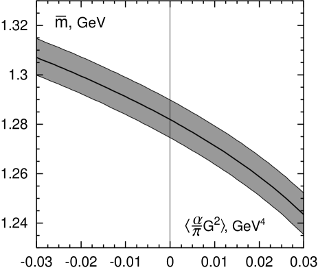
Figure 6: The dependence of $\overline{m}(\overline{m})$ on $\langle 0|\alpha s/\pi)G^{2}|0\rangle$ obtained at $n=10$,  $Q^{2}=0.98\cdot 4m^{2}$ and $\alpha_{s}(Q^{2}+\overline{m}^{2})$.

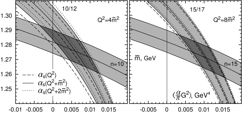
Figure 7: The dependence of $\overline{m}(\overline{m})$ on $\langle 0|(\alpha s/\pi)G^{2}|0\rangle$ obtained from the moments (horizontal bands) and their ratios (vertical bands) at different $\alpha_{s}$. The left-hand figure: $Q^{2}=4\overline{m}^{2}$,   $n=10$,   $M_{10}/M_{12}$; the right-hand figure – $Q^{2}=8\overline{m}^{2}$,   $n=15$,   $M_{15}/M_{17}$.

Functions $f^{(0)}(z)$,   $f^{(1)}(z)$ and $F(z)$ were calculated in [5], [54], [55], respectively. The use of the quark pole mass is, however, inacceptable. The matter is that in this case the PT corrections to moments are very large in the region of interest and perturbative series seems to diverge. Thus, for instance, at

$$n=10\;,\;Q^{2}=4m^{2}:\qquad{M^{(1)}\over M^{(0)}}=13.836\;,\qquad{M^{(2)}\over M^{(0)}}=193.33\;,\qquad{M^{(G,1)}\over M^{(G,0)}}=13.791$$ (66)

(here $M^{(k)}$ mean the coefficients at the contributions of terms $\sim a^{k}$ to the moments, $M^{(G,k)}$ - are the similar coefficients for gluonic condensate contribution. In the region of interest $a\sim 0.1$). At $Q^{2}=0$ the situation is even worse. So, it is reasonable to turn to to $\overline{MS}$ mass $\overline{m}(\mu^{2})$, taken at the point $\mu^{2}=\overline{m}^{2}$. After turning to the $\overline{MS}$ mass $\overline{m}(\overline{m}^{2})$ we get instead of (66):

$$n=10\;,\;Q^{2}=4{\bar{m}}^{2}:\qquad{{\bar{M}}^{(1)}\over{\bar{M}}^{(0)}}=0.045\;,\qquad{{\bar{M}}^{(2)}\over{\bar{M}}^{(0)}}=1.136\;,\qquad{{\bar{M}}^{(G,1)}\over{\bar{M}}^{(G,0)}}=-1.673$$ (67)

At $a\sim 0.1$ and at the ratios of moments given by (67) there is a good reason to believe that the PT series well converges. Such a good convergence holds (at $n>5$) only in the case of large enough $Q^{2}$, at $Q^{2}=0$ one does not succeed in finding such $n$, that perturbative corrections, $\alpha_{s}$ corrections to gluonic condensates and the term $\sim\langle G^{3}\rangle$ contribution would be simultaneously small.

It is also necessary to choose scale - normalization point $\mu^{2}$ where $\alpha_{s}(\mu^{2})$ is taken. In (64)  $R(s)$ is a physical value and cannot depend on $\mu^{2}$. Since, however, we take into account in (64) only three terms, at unsuitable choice of $\mu^{2}$ such $\mu^{2}$ dependence may arise due to neglected terms. At large $Q^{2}$ the natural choice is $\mu^{2}=Q^{2}$. It can be thought that at $Q^{2}=0$ the reasonable scale is $\mu^{2}=\overline{m}^{2}$, though some numerical factor is not excluded in this equality. That is why it is reasonable to take interpolation form

$$\mu^{2}=Q^{2}+\overline{m}^{2},$$ (68)

but to check the dependence of final results on a possible factor at $\overline{m}^{2}$. Equalling theoretical value of some moment at fixed $Q^{2}$ (in the region where $M^{(1)}_{n}$ and $M^{(2)}_{n}$ are small) to its experimental value one can find the dependence of $\overline{m}$ on $\langle(\alpha_{s}/\pi)G^{2}\rangle$ (neglecting the terms $\sim\langle G^{3}\rangle$). Such a dependence for $n=10$ and $Q^{2}/4m^{2}=0.98$ is presented in Fig.6.

To fix both $\overline{m}$ and $\langle(\alpha_{s}/\pi)G^{2}\rangle$ one should, except for moments, take their ratios. Fig.7 shows the value of $\overline{m}$ obtained from the moment $M_{10}$ and the ratio $M_{10}/M_{12}$ at $Q^{2}=4m^{2}$ and from the moment $M_{15}$ and the ratio $M_{15}/M_{17}$ at $Q^{2}=8m^{2}$. The best values of masses of charmed quark and gluonic condensate are obtained from fig.7:

$${\bar{m}}({\bar{m}}^{2})\,=\,1.275\pm 0.015\,{\rm GeV}\;,\qquad\left<{\alpha_{s}\over\pi}G^{2}\right>\,=\,0.009\pm 0.007\,{\rm GeV}^{4}$$ (69)

Up to now the corrections $\sim\langle G^{3}\rangle$ were not taken into account. It appears that in the region of $n$ and $Q^{2}$ used to find $\overline{m}$ and gluonic condensate they are comparatively small and, practically, not changing $\overline{m}$, increase $\langle((\alpha_{s}/\pi)G^{2}$ by $10-20\%$ if the term $\sim\langle G^{3}\rangle$ is estimated according to (13) at $\rho_{c}=0.5fm$.

It should be noted that improvement of the accuracy of $\Gamma_{J/\psi\to ee}$ would make it possible to precise the value of gluonic condensate: the widths of horizontal bands in fig.7 are determined mainly just by this error. In particular, this, perhaps, would allow one to exclude the zero value of gluonic condensate, that would be extremely important. Unfortunately, eq.(69) does not allow one to do it for sure. Diminution of theoreticl errors which determine the width of vertical bands seems to be less real.

6. Conclusion

In this paper I compare the results of the recent precise measurements of $\tau$-lepton hadronic decays [24]-[26] with QCD predictions in the low energy region. The perturbative terms up to $\alpha^{3}_{s}$ and the terms of the operator product expansion (OPE) up to d=8 were taken into account. It is shown that QCD with the account of OPE terms agrees with experiment up to $\sim 2\%$ at the values of the complex Borel parameter $|M^{2}|>0.8-1.0GeV^{2}$ in the left-hand semiplane of the complex plane. It was found:
1. The values of the QCD coupling constant $\alpha_{s}(m^{2}_{\tau})=0.355\pm 0.025$ from the total probability of $\tau$-decays and $\alpha_{s}(m^{2}_{\tau})=0.330$ from the sum rules at low energies. (The latter value corresponds to $\alpha_{s}(m^{2}_{z})=0.118$).
2. The value of the quark condensate square (assuming factorization)

$$\alpha_{s}\langle\mid\overline{\psi}\psi\mid 0\rangle^{2}=(2.25\pm 0.70)\cdot 10^{-4}~{}\mbox{GeV}^{6}$$

and of quark-gluon condensate of d=8.
3. The value of gluonic condensate:

a) from the $\tau$-decay data:

$$\langle 0\mid\frac{\alpha_{s}}{\pi}G^{2}\mid 0\rangle=(0.006\pm 0.012)~{}\mbox{GeV}^{4}$$

b) from the sum rules for charmonium

$$\langle 0\mid\frac{\alpha_{s}}{\pi}G^{2}\mid 0\rangle=(0.009\pm 0.007)~{}GeV^{4}$$

It is shown that the sum rules for charmonium are in agreement with experiment when accounting for perturbative corrections $\sim\alpha^{2}_{s}$ and for OPE terms proportional to $\langle(\alpha_{s}/\pi)G^{2}\rangle$ and to $\langle G^{3}\rangle$.

The main conclusion is that in the range of low-energy phenomena under consideration, perturbation theory and operator expansion, i.e. the idea of vacuum condensates in QCD is in an excellent agreement with experiment starting from $Q^{2}\sim 1GeV^{2}$.

I am deeply indebted to K.N.Zyablyuk who had made the main calculations in papers [27, 28], the results of which I used here.

The paper is supported by the grants CRDF RP2-2247, INTAS-2000-587 and RFFI 00-02-17808.

References

- [1] P.A.Aleksandrov, Akademik Anatoly Petrovich Aleksandrov: Pryamaya Rech (in Russian), Academician Anatoly Petrovich Aleksandrov: Direct speech. M.Nauka, 2001, p.177.
- [2] D.Holloway, Stalin and the bomb, Yale Univ.Press, New Haven & London, 1994, chapt.15, sec.6.
- [3] B.L.Ioffe, A top secret assignment, Novy Mir, 1999, No.6, p.161 (in Russian). English translation in: At the frontier of particle physics, Handbook of QCD, Boris Ioffe Festschrift, ed. by M.Shifman, World Svientific, 2001, v.1.
- [4] A.A.Belavin, A.M.Polyakov, A.S.Schwarz, Yu.S.Tyupkin, Phys.Lett.B, 59, 85 (1975).
- [5] M.A.Shifman, A.I.Vainstein, V.I.Zakharov, Nucl.Phys.B 147, 385,448 (1979).
- [6] V.A.Novikov, M.A.Shifman, A.I.Vainstein and V.I.Zakharov, Nucl.Phys.B 249, 445 (1985).
- [7] M.A.Shifman, Lecture at 1997 Yukawa International Seminar, Kyoto, 1997, Suppl.Prog.Theor.Phys., 1998, Vol.131, p.1.
- [8] M.Gell-Mann, R.J.Oakes, B.Renner, Phys.Rev. 175, 2195 (1968).
- [9] B.L.Ioffe, Usp.Fiz.Nauk 171, 1273 (2001).
- [10] S.Weinberg, in: A Festschrift for I.I.Rabi, Trans.New York Acad.Sci., Ser.2, Vol.38, p.185, 1977.
- [11] H.Leutwyler, Journ. Moscow Phys.Soc., 6, 1 (1996).
- [12] B.L.Ioffe, Nucl.Phys.B 188, 317 (1981); 192, 591 (1982).
- [13] H.Leutwyler in: At the Frontier of Particle Physics, Handbook of QCD, Boris Ioffe Festschrift, ed. by M.Shifman, World Scientific, Vol.1, p.271, 2001.
- [14] U.Meissner, ibid, p.417.
- [15] P.Gerber, H.Leutwyler, Nucl.Phys.B 321, 387 (1989).
- [16] P.Chen et al., Phys.Rev.D 64, 014503 (2001).
- [17] B.L.Ioffe, Lecture at St.Petersburg Winter School on Theoretical Physics, Febr.1998, Surveys in High Energy Physics, Vol.14, p.89, 1999.
- [18] V.M.Belyaev, B.L.Ioffe, ZhETF 83, 876 (1982).
- [19] V.A.Novikov, M.A.Shifman, A.I.Vainstein, V.I.Zakharov, Phys.Lett.B 86, 347 (1979).
- [20] B.L.Ioffe, A.V.Smilga, Nucl.Phys.B 232, 109 (1984).
-
[21]
V.M.Belyaev, Ya.I.Kogan, Yad.Fiz. 40,
1035 (1984).
I.I.Balitsky, A.V.Kolesnichenko, A.V.Yung, Yad.Fiz. 41, 282 (1985). - [22] V.M.Belyaev, Ya.I.Kogan, Pis’ma v ZhETF 37, 611 (1983).
- [23] B.L.Ioffe, A.G.Oganesian, Phys.Rev.D 57, R6590 (1998).
- [24] ALEPH Collaboration, R.Barate et al., Eur.Phys.J.C 4, 409 (1998).
- [25] OPAL Collaboration, K.Ackerstaff et al., Eur.Phys.J.C 7, 571 (1999); G.Abbiendi et al., ibid, 13, 197 (2002).
- [26] CLEO Collaboration, S.J.Richichi et al., Phys.Rev.D 60, 112002 (1999).
- [27] B.L.Ioffe, K.N.Zyablyuk, Nucl.Phys.A 687, 437 (2001).
- [28] B.V.Geshkenbein, B.L.Ioffe, K.N.Zyablyuk, Phys.Rev.D 64, 093009 (2001).
- [29] A.Pich, Proc. of QCD94 Workshop, Monpellier, 1944; Nucl.Phys.B (proc.Suppl) 39, 396 (1995).
- [30] W.J.Marciano, A.Sirlin, Phys.Rev.Lett. 61, 1815 (1988).
- [31] E.Braaten, Phys.Rev.Lett. 60, 1606 (1988); Phys.Rev.D 39, 1458 (1989).
- [32] S.Narison, A.Pich, Phys.Lett.B 211, 183 (1988).
- [33] F.Le Diberder, A.Pich, Phys.Lett.B 286, 147 (1992).
- [34] K.G.Chetyrkin, A.L.Kataev, F.V.Tkachov, Phys.Lett.B 85, 277 (1979); M.Dine, J.Sapirshtein, Phys.Rev.Lett. 43 668 (1979); W.Celmaster, R.Gonsalves, ibid, 44, 560 (1980).
-
[35]
L.R.Surgaladze,
M.A.Samuel, Phys.Rev.Lett. 66, 560 (1991);
S.G.Goryshny, A.L.Kataev, S.A.Larin, Phys.Lett.B 259, 144 (1991). - [36] A.L.Kataev, V.V.Starshenko, Mod.Phys.Lett.A 10, 235 (1995).
- [37] O.V.Tarasov, A.A.Vladimirov, A.Yu.Zharkov, Phys.Lett.B 93, 429 (1980); S.A.Larin, J.A.M.Vermaseren, ibid, 303, 334 (1993).
- [38] T.van Ritbergen, J.A.M.Vermaseren, S.A.Larin, Phys.Lett.B 400, 379 (1997).
- [39] K.G.Chetyrkin, S.G.Gorishny, V.P.Spiridonov, Phys.Lett.B 160, 149 (1985).
- [40] L.-E.Adam, K.G.Chetyrkin, Phys.Lett.B 329, 129 (1994).
- [41] E.Braaten, C.S.Lee, Phys.Rev.D 42, 3888 (1990).
- [42] K.Hagiwara et al., Particle Data Groop, Phys.Rev.D 66, 010001 (2002).
- [43] ALEPH Collaboration, R.Barate et al., Eur.Phys.J.C 11, 599 (1999).
- [44] OPAL Collaboration, G.Abbiendi et al., Eur.Phys.J.C 19, 653 (2001).
- [45] I.L. Solovtsov, D.V.Shirkov, Phys.Rev.Lett. 79, 1209 (1997), Teor.Mat.Fiz. 120, 1210 (1999).
- [46] B.V.Geshkenbein, B.L.Ioffe, Pis’ma v ZhETF, 70, 167 (1999).
- [47] K.G.Chetyrkin, S.Narison, V.I.Zakharov, Nucl.Phys.B 550, 353 (1999).
- [48] T.Shafer, E.V.Shuryak, Rev.Mod.Phys. 70, 323 (1998).
- [49] B.L.Ioffe, K.N.Zyablyuk, hep-ph/0207183.
- [50] V.B.Berestetsky, I.Ya.Pomeranchuk, JETP 29, 864 (1955).
- [51] J.Schwinger, Particles, Sources, Fields, Addison-Wesley Publ., 1973, V.2.
-
[52]
A.H.Hoang, J.H.Kuhn, T.Teubner,
Nucl.Phys.B 452, 173 (1995);
K.G.Chetyrkin, J.H.Kuhn, M.Steinhauser, Nucl.Phys.B 482, 213 (1996);
K.G.Chetyrkin et al., Nucl.Phys.B 503, 339 (1997);
K.G.Chetyrkin et al., Eur.Phys.J.C 2, 137 (1998). - [53] D.J.Broadhurst et al., Phys.Lett.B 329, 103 (1994).
- [54] S.N.Nikolaev, A.V.Radyushkin, Yad.Fiz. 39, 147 (1984).