hep-ph/0207189

July, 2002

Vector-meson contributions do not explain the rate and spectrum in $K_{L}\rightarrow\pi^{0}\gamma\gamma$

F. Gabbiani and G. Valencia

Department of Physics and Astronomy, Iowa State University, Ames, Iowa 50011

We analyze the recent NA48 data for the reaction $K_{L}\rightarrow\pi^{0}\gamma\gamma$ with and without the assumption of vector meson dominance (VMD). We find that the data are well described by a three-parameter expression inspired by ${\cal O}(p^{6})$ chiral perturbation theory. We also find that it is impossible to fit the shape of the decay distribution and the overall rate simultaneously if one imposes the VMD constraints on the three parameters. We comment on the different fits and their implications for the $CP$-conserving component of the decay $K_{L}\rightarrow\pi^{0}e^{+}e^{-}$.

1 Introduction

In Ref. [1] we examined the KTeV [2] data for the mode $K_{L}\rightarrow\pi^{0}\gamma\gamma$ using a more general (three-parameter) description than the one used by KTeV. The latter has become the norm in the literature and it follows from an assumption of vector meson dominance (VMD) [3] in conjunction with the parametrization inspired by ${\cal}O(p^{6})$ chiral perturbation theory of Ref. [4]. We argued that VMD in this decay is an experimental question and, therefore, that it should not be an input to the data analysis. We found a least squares best fit to the data within our approach that was slightly better than the usual fit. However, it was hard to reach definitive conclusions because the necessary information is not made available by KTeV. Nevertheless, we motivated our more general approach by showing that there are important contributions to this decay from intermediate $f^{\phantom{l}}_{2}(1270)$ mesons that do not conform to the VMD parametrization [5].

In this paper we present our three-parameter fit for newly released data from NA48 [6]. This is important for the following reasons. First, the NA48 data are significantly different from the KTeV data and leads to different conclusions regarding the $CP$-conserving contribution to $K_{L}\rightarrow\pi^{0}e^{+}e^{-}$ [7]–[9]. Second, NA48 has presented their data in a form that allows us to directly compare our general fit to the usual VMD fit. This allows us to show that whereas it is possible to fit the decay distribution $d\Gamma/dm_{\gamma\gamma}$ equally well with the general and VMD approaches, only the former is capable of fitting simultaneously the decay distribution and the total decay rate.

We also discuss two additional issues. First, we show that the two fits to the decay distribution (the general and the VMD parametrizations) correspond respectively to constructive and destructive interference between two amplitudes. Second, we comment on the dependence of the fit on the parameter $a^{\phantom{l}}_{2}$, which is extracted from $K\rightarrow\pi\pi\pi$ decays and which has a large uncertainty [10, 11].

2 Parametrization of the data

The $K_{L}\rightarrow\pi^{0}\gamma\gamma$ amplitude in the limit of $CP$ violation can be written in terms of two independent invariant amplitudes, A and B [8],

$${\cal M}[K_{L}(p^{\phantom{l}}_{K})\rightarrow\pi^{0}(p^{\phantom{l}}_{\pi})\gamma(q^{\phantom{l}}_{1})\gamma(q^{\phantom{l}}_{2})]\,=\,{G^{\phantom{l}}_{8}\alpha^{\phantom{l}}_{EM}\over 4\pi}\epsilon^{\phantom{l}}_{\mu}(q^{\phantom{l}}_{1})\,\epsilon^{\phantom{l}}_{\nu}(q^{\phantom{l}}_{2})\,\Bigg{[}A\,\left(q_{2}^{\mu}q_{1}^{\nu}-q^{\phantom{l}}_{1}\cdot q^{\phantom{l}}_{2}\,g^{\mu\nu}\right)$$ (1)

$$+2{B\over{m^{2}_{K}}}\,\left(p^{\phantom{l}}_{K}\cdot q^{\phantom{l}}_{1}\,q_{2}^{\mu}p_{K}^{\nu}+p^{\phantom{l}}_{K}\cdot q^{\phantom{l}}_{2}\,q_{1}^{\nu}p_{K}^{\mu}-q^{\phantom{l}}_{1}\cdot q^{\phantom{l}}_{2}\,p_{K}^{\mu}p_{K}^{\nu}-p^{\phantom{l}}_{K}\cdot q^{\phantom{l}}_{1}\,p^{\phantom{l}}_{K}\cdot q^{\phantom{l}}_{2}\,g^{\mu\nu}\right)\Bigg{]}\;.$$

The Fermi constant and the Cabibbo angle are included in the overall constant $G^{\phantom{l}}_{8}=9.1\times 10^{-6}$ GeV^-2 and $\alpha^{\phantom{l}}_{EM}\approx 1/137$ is the usual electromagnetic fine structure constant. To parametrize these amplitudes in a form inspired by ${\cal O}(p^{6})$ chiral perturbation theory and dispersion relations Ref. [4] proposed the use of:

$$A(z,y) = 4F\left(\frac{z}{r^{2}_{\pi}}\right){a^{\phantom{l}}_{1}(z)\over z}+4{F(z)\over z}(1+r^{2}_{\pi}-z)$$

$$+ {a^{\phantom{l}}_{2}M^{2}_{K}\over{\Lambda^{2}_{\chi}}}\left\{{4r^{2}_{\pi}\over z}F\left(\frac{z}{r^{2}_{\pi}}\right)+{2\over 3}\left(2+\frac{z}{r^{2}_{\pi}}\right)\left[{1\over 6}+R\left(\frac{z}{r^{2}_{\pi}}\right)\right]-{2\over 3}\log{m^{2}_{\pi}\over M^{2}_{\rho}}\right.$$

$$- 2\frac{r^{2}_{\pi}}{z^{2}}(z+1-r^{2}_{\pi})^{2}\left[\frac{z}{12r^{2}_{\pi}}+F\left(\frac{z}{r^{2}_{\pi}}\right)+\frac{z}{r^{2}_{\pi}}R\left(\frac{z}{r^{2}_{\pi}}\right)\right]$$

$$+ \left.8\frac{r^{2}_{\pi}}{z^{2}}y^{2}\left[\frac{z}{12r^{2}_{\pi}}+F\left(\frac{z}{r^{2}_{\pi}}\right)+\frac{z}{2r^{2}_{\pi}}F\left(\frac{z}{r^{2}_{\pi}}\right)+3\frac{z}{r^{2}_{\pi}}R\left(\frac{z}{r^{2}_{\pi}}\right)\right]\right\}$$

$$+ \alpha^{\phantom{l}}_{1}(z-r^{2}_{\pi})+\alpha^{\phantom{l}}_{2}\;,$$

$$B(z) = {a^{\phantom{l}}_{2}M^{2}_{K}\over{\Lambda^{2}_{\chi}}}\left\{{4r^{2}_{\pi}\over z}F\left(\frac{z}{r^{2}_{\pi}}\right)+{2\over 3}\left(10-\frac{z}{r^{2}_{\pi}}\right)\left[{1\over 6}+R\left(\frac{z}{r^{2}_{\pi}}\right)\right]+{2\over 3}\log{m^{2}_{\pi}\over m^{2}_{\rho}}\right\}+\beta\;,$$ (2)

where the dimensionless kinematic variables are

$$z={\left(q^{\phantom{l}}_{1}+q^{\phantom{l}}_{2}\right)^{2}\over M^{2}_{K}}\;,\ \ y={p^{\phantom{l}}_{K}\cdot(q^{\phantom{l}}_{1}-q^{\phantom{l}}_{2})\over M^{2}_{K}}\;,$$ (3)

and the scale of chiral symmetry breaking is $\Lambda^{\phantom{l}}_{\chi}$ $\approx$ $4\pi f^{\phantom{l}}_{\pi}$ $\approx$ 1.17 GeV.

The form in Eq. (2) does not correspond to a complete calculation at order $p^{6}$ in chiral perturbation theory. Rather it contains the complete one-loop calculation at order $p^{4}$ [12] and two additional ingredients containing some corrections of order $p^{6}$ [13, 4]. The non-analytic terms in Eq. (2) that multiply the factors $a^{\phantom{l}}_{2}$ and $a^{\phantom{l}}_{1}(z)$ attempt to incorporate the strong rescattering in the two-pion intermediate state that occurs at one-loop. They arise from the inclusion of $p^{4}$ corrections to the $K\rightarrow 3\pi$ amplitudes [10, 14]. The values of $a^{\phantom{l}}_{1}$ and $a^{\phantom{l}}_{2}$ are extracted from data and the functions $F(z)$ and $R(z)$ can be found in the literature [4]. The three constants $\alpha^{\phantom{l}}_{1}$, $\alpha^{\phantom{l}}_{2}$ and $\beta$ originate in counterterms appearing in the $p^{6}$ weak chiral Lagrangian [4].

The analysis of $K\rightarrow 3\pi$ in Ref.  [10] indicates that

$$a^{\phantom{l}}_{1}(z)=0.38+0.13\;Y^{\phantom{l}}_{0}-0.0059\;Y^{2}_{0}\;, a^{\phantom{l}}_{2}=6.5\;,$$

$$Y^{\phantom{l}}_{0}={(z-r^{2}_{\pi}-{1\over 3})\over r^{2}_{\pi}}\;, r^{\phantom{l}}_{\pi}=m^{\phantom{l}}_{\pi}/M^{\phantom{l}}_{K}\;.$$ (4)

A very recent analysis of $K\rightarrow 3\pi$ data results in [11]

$$a^{\phantom{l}}_{2}=6.8\pm 2.4\;.$$ (5)

In the analysis of Ref. [4], which has become standard, the three unknown constants were fixed in terms of the contribution they receive from vector-meson exchange, supplemented with a minimal subtraction ansatz:

$$\alpha^{\phantom{l}}_{1} = -4a^{\phantom{l}}_{V}\;,$$

$$\alpha^{\phantom{l}}_{2} = 12a^{\phantom{l}}_{V}-0.65\;,$$

$$\beta = -8a^{\phantom{l}}_{V}-0.13\;,$$ (6)

and this form has been used both by KTeV [2] and by NA48 [6] to fit their data. In Ref. [1] we argued that this ansatz imposes a correlation on $\beta$ that is not desirable for a prediction of the $CP$-conserving contribution to $K_{L}\rightarrow\pi^{0}e^{+}e^{-}$. With the new NA48 data we can go further and conclude that the VMD ansatz does not provide a good description of $K_{L}\rightarrow\pi^{0}\gamma\gamma$.

3 Fitting the shape of the $d\Gamma/dm_{\gamma\gamma}$ distribution

NA48 has recently released their result for $K_{L}\rightarrow\pi^{0}\gamma\gamma$ [6]. They chose to analyze their data using Eq. (2) with the VMD assumption, and they found $a^{\phantom{l}}_{V}=-0.46$. To obtain this number they fit the shape of the distribution $d\Gamma/dydm_{\gamma\gamma}$ without attempting to fit the branching ratio. NA48 has published in Table 2 of Ref. [6] sufficient information to fit the distribution $d\Gamma/dm_{\gamma\gamma}$. They present the number of unambiguous events, estimated background and acceptance for each 20 MeV bin in $m^{\phantom{l}}_{\gamma\gamma}$.

We begin our analysis with a fit to the shape of the $d\Gamma/dm_{\gamma\gamma}$ distribution, ignoring the measured branching ratio, to compare with the fit performed by NA48. We do this both using the VMD assumption and with the general approach. We calculate the number of events predicted in each bin as

$$N_{i}=N\biggl{[}{1\over\Gamma_{K_{L}}}\int_{i}dm_{\gamma\gamma}\biggl{(}{d\Gamma\over dm_{\gamma\gamma}}\biggr{)}N(K_{L})\biggr{]}{\rm Acceptance}_{i}+{\rm Background}_{i}\;,$$ (7)

where $N$ is a normalization chosen to match the total number of events and $N(K_{L})$ = 23.9 $\times$ 10⁹ is the number of decays in the fiducial volume. The arbitrary normalization allows us to fit the shape of the distribution while ignoring the overall rate.

We use data from 17 out of 20 bins presented in Table 2 of Ref. [6]. We exclude two bins in the $m^{\phantom{l}}_{\gamma\gamma}$ region near the $\pi^{0}$ mass which do not have any events due to kinematic cuts, and we also exclude the last bin with no events because it lies outside the physical region. We perform a least squares fit using Poisson statistics for the bins with small number of events following Ref. [15].

With this procedure, and the VMD ansatz, we reproduce approximately the NA48 best fit. We obtain $a^{\phantom{l}}_{V}=-0.455$ with a $\chi^{2}/dof=18.5/16$. We show this result in Fig. 1 where we superimpose our best three-parameter fit which has a $\chi^{2}/dof=14.6/14$. The two fits are nearly identical as can be seen in the figure and they are indistinguishable statistically. Nevertheless, when they are both expressed in terms of the three general parameters one can see they correspond to very different solutions. For the general fit,

$$\alpha^{\phantom{l}}_{1}=4.57\;,\qquad\alpha^{\phantom{l}}_{2}=-3.89\;,\qquad\beta=0.75\;;$$ (8)

whereas for the VMD fit (in terms of $a^{\phantom{l}}_{V}$),

$$\alpha^{\phantom{l}}_{1}=1.82\;,\qquad\alpha^{\phantom{l}}_{2}=-6.10\;,\qquad\beta=3.51\;.$$ (9)

Figure 1: Two different fits to the data from Ref. [6], as explained in the text. The solid line is a one-parameter fit corresponding to Eq. (9), the dashed line is the three-parameter fit shown in Eq. (8).

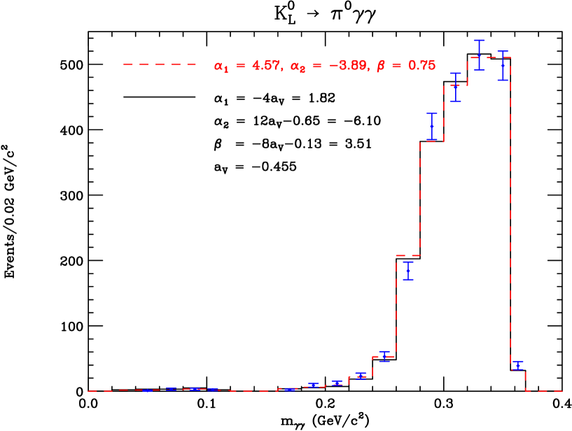
For the case of the three-parameter fit we find that $\alpha^{\phantom{l}}_{1}$ and $\alpha^{\phantom{l}}_{2}$ are correlated as was discussed in Ref. [1], so that there are many other fits with a $\chi^{2}$ near the minimum for the same value of $\beta$.

As stated above, neither one of these fits reproduces the experimental rate, $B(K_{L}\rightarrow\pi^{0}\gamma\gamma)=(1.36\pm 0.03\pm 0.03)\times 10^{-6}$ [6]. The theoretical branching ratio predicted for $a^{\phantom{l}}_{V}=-0.455$ (the NA48 value) is $B(K_{L}\rightarrow\pi^{0}\gamma\gamma)=1.1\times 10^{-6}$, and the one predicted for the three parameters in Eq. (8) is $B(K_{L}\rightarrow\pi^{0}\gamma\gamma)=1.0\times 10^{-6}$.

It is instructive to show the three separate contributions that result from Eq. (2) to the differential decay rate $dB(K_{L}\rightarrow\pi^{0}\gamma\gamma)/dm_{\gamma\gamma}$. The three terms correspond to the absolute square of the $A$ and $B$ amplitudes and to their interference, $|A|^{2}$, $|B|^{2}$ and ${\rm Re}(A^{\star}B)$, respectively. We show these quantities in Fig. 2 for the best three-parameter fit and Fig. 3 for the best $a^{\phantom{l}}_{V}$ fit.

Figure 2: The contributions from $|A|^{2}$ (solid line), $|B|^{2}$ (dashed line), and Re($A^{\star}B$) (dot-dashed line) are plotted vs. the invariant two-photon mass $m_{\gamma\gamma}$ in terms of the number of events for the best three-parameter fit.

Figure 3: Same as in Fig. 2 for the best $a_{V}$ fit.

In both of these figures the solid line represents the contribution from $|A|^{2}$, the dashed line the contribution from $|B|^{2}$ and the dot-dashed line the interference. We observe that the three-parameter fit corresponds to constructive interference between the $A$ and $B$ amplitudes, whereas the $a^{\phantom{l}}_{V}$ fit corresponds to destructive interference. Unfortunately it appears that it is not possible to determine experimentally the sign of this interference. However, as we show below, the total rate for the process discriminates between the VMD ansatz and the general form of the amplitude.

4 Simultaneous fit to the shape of the $d\Gamma/dm_{\gamma\gamma}$ distribution and to the decay rate

To obtain a fit that reproduces the observed branching ratio we proceed as in Eq. (7) but removing the arbitrary normalization,

$$N_{i}=\biggl{[}{1\over\Gamma_{K_{L}}}\int_{i}dm_{\gamma\gamma}\biggl{(}{d\Gamma\over dm_{\gamma\gamma}}\biggr{)}N(K_{L})\biggr{]}{\rm Acceptance}_{i}+{\rm Background}_{i}\;,$$ (10)

with the same notation of Eq. (7). We first attempt this fit with the VMD ansatz and find that it is impossible to obtain a good fit. Our least squares fit using the VMD ansatz occurs for $a^{\phantom{l}}_{V}=-0.63$ and has a $\chi^{2}/dof=74.8/16$. We show this result as the solid line in Figs. 4 and 5. The implied branching ratio is $B(K_{L}\rightarrow\pi^{0}\gamma\gamma)=1.25\times 10^{-6}$ and $a^{\phantom{l}}_{V}=-0.63$ corresponds to

$$\alpha^{\phantom{l}}_{1}=2.51\;,\qquad\alpha^{\phantom{l}}_{2}=-8.19\;,\qquad\beta=4.89\;.$$ (11)

Figure 4: A simultaneous fit to the shape of $d\Gamma/dm_{\gamma\gamma}$ and to the decay rate. The solid line is a one-parameter fit corresponding to Eq. (11), the dashed line is the three-parameter fit shown in Eq. (12).

Figure 5: An enlargement of Fig. 4 for $m_{\gamma\gamma}\leq 0.24$ GeV/c².

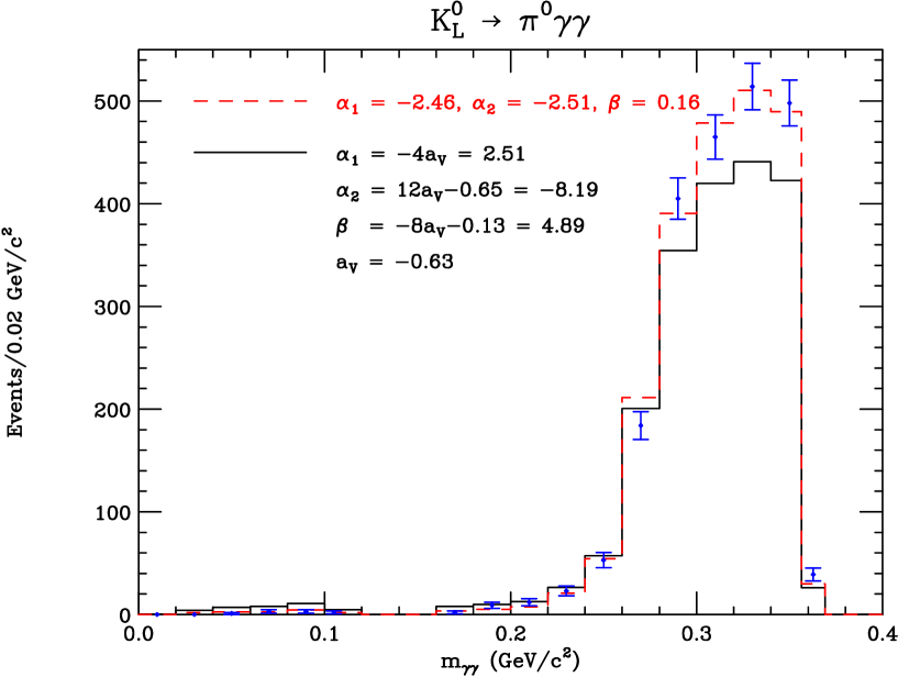
Our best three-parameter fit, on the other hand, has a $\chi^{2}/dof=18.5/14$ and is shown as the dashed line in Figs. 4 and 5. It implies a branching ratio $B(K_{L}\rightarrow\pi^{0}\gamma\gamma)=1.36\times 10^{-6}$ in good agreement with the measured one. The parameters for this best fit are,

$$\alpha^{\phantom{l}}_{1}=-2.46\;,\qquad\alpha^{\phantom{l}}_{2}=-2.51\;,\qquad\beta=0.16\;.$$ (12)

We conclude from Fig. 4 that the VMD ansatz cannot reproduce the shape of the spectrum and the total decay rate simultaneously, but that the general formula, Eq. (2) does accommodate both.

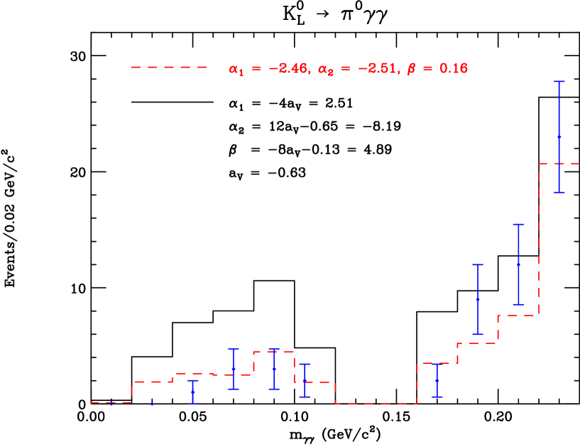
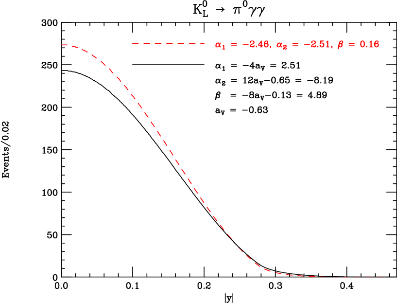
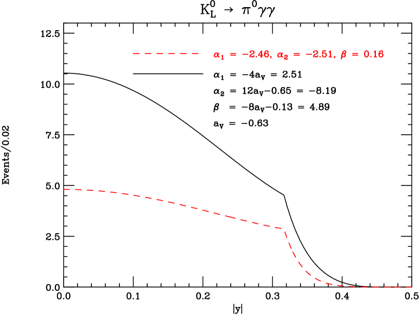
For completeness we show in Figs. 6 and 7 the theoretical $d\Gamma/dy$ distributions for both the $a^{\phantom{l}}_{V}$ result from Eq. (11) and the three parameters given in Eq. (12). Fig. 7 is restricted to events with $m_{\gamma\gamma}\leq 0.24$ GeV/c². There are no data available in this form, so at this point we are not able to perform a fit and we can only present our predictions. We point out that the three-parameter fit yields a flatter distribution than the $a^{\phantom{l}}_{V}$ fit.

Figure 6: Theoretical $d\Gamma/dy$ distributions. The solid and dashed lines are predicted using as input the results given in Eq. (11) and Eq. (12), respectively.

Figure 7: Same as Fig. 6 but with a cut at $m_{\gamma\gamma}\leq 0.24$ GeV/c².

4.1 Dependence on $a_{2}$

We now consider the dependence of our results on the parameter $a^{\phantom{l}}_{2}$ that appears in the $B$ amplitude. This parameter is extracted from $K\rightarrow 3\pi$ decays and up to now we have used the value $a^{\phantom{l}}_{2}=6.5~{}\cite[cite]{[\@@bibref{}{unitco}{}{}]}$. However, the value of this parameter has a large uncertainty, of order $\sim 35\,\%$. For example, from the recent analysis of Ref. [11] one extracts $a^{\phantom{l}}_{2}=6.8\pm 2.4$.

The analytic form for the $B$ amplitude in Eq. (2) clearly indicates that $a^{\phantom{l}}_{2}$ and $\beta$ are correlated and this is confirmed by our numerical study. It is possible to obtain many equally good fits to the data with different values of $a^{\phantom{l}}_{2}$ and $\beta$. For example if we take the central value from Ref. [11] and 1-sigma deviations from it, we find good fits to the shape and spectrum with the values listed in Table 1. This is not possible with the $a^{\phantom{l}}_{V}$ parametrization, where we cannot find a good fit for any of these values of $a^{\phantom{l}}_{2}$.

$a^{\phantom{l}}_{2}$	$\alpha^{\phantom{l}}_{1}$	$\alpha^{\phantom{l}}_{2}$	$\beta$	$\chi^{2^{\phantom{l}}}/dof$
6.8	–2.42	–2.65	0.25	18.5/14
4.4	–2.33	–1.71	–0.46	18.4/14
9.2	–2.58	–3.51	0.91	18.6/14

Table 1: Three-parameter best fits for three different values of $a_{2}$, corresponding to its central value from Ref. [11] and its 1-sigma deviations.

5 $CP$-conserving contribution to $K_{L}\rightarrow\pi^{0}e^{+}e^{-}$

We now turn to the estimate of the $CP$-conserving contribution to $K_{L}\rightarrow\pi^{0}e^{+}e^{-}$ using the model of Ref. [9]. Using the results of the fit to the shape of the distribution only, Eqs. (9) and (8), we find

$$B_{CPC}(K_{L}\rightarrow\pi^{0}e^{+}e^{-})=\cases{4.0\times 10^{-13}&{\rm vector meson dominance}\cr 2.0\times 10^{-13}&{\rm three-parameter~{}fit .}\cr}$$ (13)

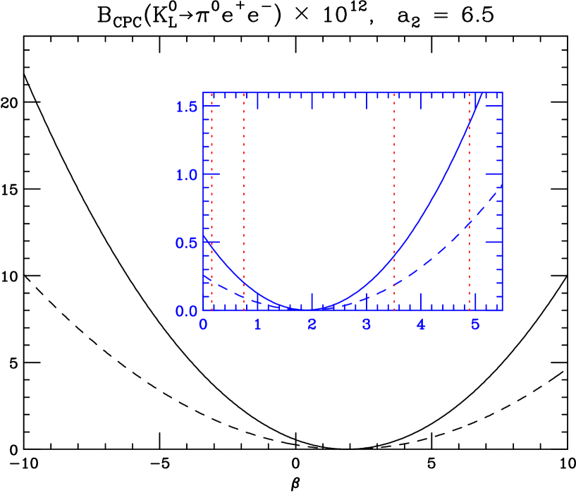
Notice that these two numbers are an order of magnitude smaller than what is obtained using the KTeV data instead (see Eq. (11) of Ref. [1]). We can see from Fig. 8 why the NA48 result [6] implies a much smaller $B_{CPC}(K_{L}\rightarrow\pi^{0}e^{+}e^{-})$ than the KTeV result [2] ($\beta=-5$ for the three-parameter fit or $\beta=7.5$ for the $a^{\phantom{l}}_{V}$ fit). These two points are shown as the two internal dotted lines in Fig. 8. It is clear from this figure that the NA48 results correspond to a $K_{L}\rightarrow\pi^{0}\gamma\gamma$ that produces a minimal $CP$-conserving contribution in $K_{L}\rightarrow\pi^{0}e^{+}e^{-}$, i.e. it indicates that the two photons have a negligible D-wave component. The VMD result in Eq. (13) is consistent with the result reported by NA48. The latter is based on an analysis of the low $m^{\phantom{l}}_{\gamma\gamma}$ region only and yields $B_{CPC}(K_{L}\rightarrow\pi^{0}e^{+}e^{-})=(4.7^{+2.2}_{-1.8})\times 10^{-13}$ [6]. The NA48 result is obtained from data with $m^{\phantom{l}}_{\gamma\gamma}$ below 110 MeV and is therefore model independent because in that region the $B$ amplitude dominates and the correlation with the $A$ amplitude implied by the VMD ansatz disappears.

Figure 8: $CP$-conserving contribution to $K_{L}\rightarrow\pi^{0}e^{+}e^{-}$ as a function of $\beta$ with $a_{2}$ = 6.5 [4]. The dashed line shows the absorptive contribution and the solid line the model of Ref. [9]. The enlargement shows the results for the branching ratio vs. the four values of $\beta$ = 0.16, 0.75, 3.51 and 4.89 from the three- and one-parameter fits discussed in the text. These are marked by vertical dotted lines.

If we use the results of the fits to both rate and spectrum, Eqs. (11) and (12), we find instead,

$$B_{CPC}(K_{L}\rightarrow\pi^{0}e^{+}e^{-})=\cases{(13.8^{+0.9}_{-2.1})\times 10^{-13}&{\rm vector meson dominance}\cr(4.6^{+1.7}_{-2.2})\times 10^{-13}&{\rm three-parameter~{}fit .}\cr}$$ (14)

These two points are shown as the external dotted lines in Fig. 8. Not surprisingly, the general three-parameter fit continues to agree with the model independent NA48 limit as it gives a good fit to both the rate and spectrum. On the other hand, the fit in terms of $a^{\phantom{l}}_{V}$ alone does not reproduce the data very well and we can dismiss its implication of a larger $B_{CPC}(K_{L}\rightarrow\pi^{0}e^{+}e^{-})$.

In Fig. 8 we see why there are two different solutions for $\beta$ that result in the same $B_{CPC}(K_{L}\rightarrow\pi^{0}e^{+}e^{-})$. This $CP$-conserving component depends quadratically on the $B(z)$ amplitude of $K_{L}\rightarrow\pi^{0}\gamma\gamma$, and therefore there are two values of $\beta$ for any given $B_{CPC}(K_{L}\rightarrow\pi^{0}e^{+}e^{-})$. They correspond to constructive and destructive interference between the term with $a^{\phantom{l}}_{2}$ and $\beta$ in Eq. (2).

6 Conclusion

We have shown that the NA48 data for the reaction $K_{L}\rightarrow\pi^{0}\gamma\gamma$ can be accommodated nicely by the theoretical expression based on chiral perturbation theory at order $p^{6}$. With this expression it is possible to describe simultaneously the total rate and the shape of the spectrum, which is not possible with chiral perturbation theory at order $p^{4}$ [16]. We have also shown that the commonly used VMD ansatz fails in this case, and that it is impossible to fit both the rate and the shape of the spectrum if this ansatz is adopted.

We have also shown that it is possible to obtain a good fit to this mode for different values of the poorly known parameter $a^{\phantom{l}}_{2}$ from $K\rightarrow 3\pi$ decays. This indicates both that $K_{L}\rightarrow\pi^{0}\gamma\gamma$ cannot provide additional information on the value of $a^{\phantom{l}}_{2}$, and that not knowing its precise value does not affect our ability to describe the features of $K_{L}\rightarrow\pi^{0}\gamma\gamma$.

Although we do not have sufficient information to perform a similar comparison for the KTeV data, we note that the value of $a^{\phantom{l}}_{V}$ reported by KTeV [2], $a^{\phantom{l}}_{V}=-0.72\pm 0.05\pm 0.06$ predicts a branching ratio $B(K_{L}\rightarrow\pi^{0}\gamma\gamma)=(1.36\pm 0.06\pm 0.07)\times 10^{-6}$ in conflict with the measured value, $B(K_{L}\rightarrow\pi^{0}\gamma\gamma)=(1.68\pm 0.07\pm 0.08)\times 10^{-6}$.

The new results from NA48 indicate a very small D-wave component for the photon pair and this leads to a prediction of a negligible $CP$-conserving background to $K_{L}\rightarrow\pi^{0}e^{+}e^{-}$. We have shown that this result is not an artifact of the VMD ansatz and that it holds in the general parametrization. This result is at odds with the earlier KTeV data and we must wait for the new KTeV results to see how this discrepancy is resolved.

References

• [1] F. Gabbiani and G. Valencia, Phys. Rev. D 64, 094008 (2001) [hep-ph/0105006].
• [2] KTeV Collaboration, A. Alavi-Harati et al. Phys. Rev. Lett. 83, 917 (1999) [hep-ex/9902029].
• [3] G. Ecker, A. Pich, and E. de Rafael, Phys. Lett. B 237, 481 (1990); L. M. Sehgal, Phys. Rev. D 41, 161 (1990); P. Ko and J. L. Rosner, ibid. 40, 3775 (1989); P. Ko, ibid. 41, 1531 (1990).
• [4] A. G. Cohen, G. Ecker, and A. Pich, Phys. Lett. B 304, 347 (1993).
• [5] Other contributions are also discussed in J. Bijnens, S. Dawson, and G. Valencia, Phys. Rev. D 44, 3555 (1991); S. Fajfer, ibid. 51, 1101 (1995) [hep-ph/9406377]; Nuovo Cimento A 109, 1439 (1996).
• [6] NA48 Collaboration, A. Lai et al. hep-ex/0205010.
• [7] J. F. Donoghue, B. R. Holstein, and G. Valencia, Phys. Rev. D 35, 2769 (1987); L. M. Sehgal, ibid. 38, 808 (1988); P. Heiliger and L. M. Sehgal, ibid. 47, 4920 (1993); J. Kambor and B. R. Holstein, ibid. 49, 2346 (1994) [hep-ph/9310324]; Some reviews of this and other kaon decay modes are J. L. Ritchie and S. G. Wojcicki, Rev. Mod. Phys. 65, 1149 (1993); L. Littenberg and G. Valencia, Annu. Rev. Nucl. Part. Sci. 43, 729 (1993) [hep-ph/9303225]; G. D’Ambrosio and G. Isidori, Int. J. Mod. Phys. A 13, 1 (1998) [hep-ph/9611284]; A. R. Barker and S. H. Kettell, Annu. Rev. Nucl. Part. Sci. 50, 249 (2000) [hep-ex/0009024].
• [8] G. Ecker, A. Pich, and E. de Rafael, Nucl. Phys. B303, 665 (1988).
• [9] J. F. Donoghue and F. Gabbiani, Phys. Rev. D 51, 2187 (1995) [hep-ph/9408390].
• [10] J. Kambor, J. Missimer, and D. Wyler, Phys. Lett. B 261, 496 (1991).
• [11] J. Bijnens, P. Dhonte, and F. Persson, hep-ph/0205341.
• [12] G. Ecker, A. Pich, and E. de Rafael, Phys. Lett. B 189, 363 (1987); L. Cappiello and G. D’Ambrosio, Nuovo Cimento A 99, 153 (1988).
• [13] L. Cappiello, G. D’Ambrosio, and M. Miragliuolo, Phys. Lett. B 298, 423 (1993).
• [14] J. F. Donoghue, E. Golowich, and B. R. Holstein, Phys. Rev. D 30, 587 (1984).
• [15] G. J. Feldman and R. D. Cousins, Phys. Rev. D 57, 3873 (1998) [physics/9711021].
• [16] NA31 Collaboration, G. D. Barr et al. Phys. Lett. B 242, 523 (1990); 284, 440 (1992); 328, 528 (1994); E731 Collaboration, V. Papadimitriou et al. Phys. Rev. D 44, 573 (1991).